行政院國家科學委員會專題研究計畫成果報告
虛擬實境中結合幾何與影像顯像技術之研究 (II)
Hybr id Render ing Techniques for Vir tual Reality (II)
計畫編號:NSC 90-2213-E-009-126
執行期限:90 年 8 月 1 日至 91 年 7 月 31 日
主持人:莊榮宏
交通大學資工系
1. 中文摘要
這個計劃結合了幾何以及影像是顯像技術,發展 出一套整合式顯像系統以即時地瀏覽複雜的虛擬實 境。這個系統分成兩個階段,前置處理階段包含了場 景分割、依據物體自身遮擋選擇其表示法、保守的背 向剔除以及保守的可見性剔除。目的都是要盡量降低 瀏覽時的場景複雜度。在執行階段,針對深度網格採 用貼圖的方式來加速顯像,而執行期的可見性剔除也 能輕易地整合到我們的系統中。我們的實驗結果顯示 了我們的系統只損失少許的影像品質,便能以即時的 顯像率來瀏覽相當複雜的場景。 關鍵詞:虛擬實境、可見性剔除、影像快取、影像式 顯像、混合式顯像Abstr act
In this project, we combine geometry-based and image-based rendering techniques to develop a VR navigation system that aims to have efficiency relatively independent of the scene complexity. The system has two stages. The pre-processing stage includes 3D scene partitioning, object representation selection depending on its self-occlusion error, conservative back-face computation, and conservative visibility computation. All aim to remove polygons that are invisible from any point inside the cell. At run-time stage, LOD meshes are rendered normally while depth meshes are rendered by texture mapping with their cached images. Techniques for run-time back-face culling and occlusion culling can be easily included. Our experimental results have depicted fast frame rates for complex environments with an acceptable quality-loss.
Keywor ds: Virtual Reality, Visibility, Image Caching, Image-Based Rendering, Hybrid Rendering
2. INTRODUCTION
To take the advantages of both geometry- and image-based rendering techniques, we introduce a hybrid rendering scheme that aims to render a complex scene in a constant and high frame rate with only a little or an acceptable quality loss. The hybrid scheme consists of two stages: pre-processing stage and run-time stage. In the pre-processing stage, to exploit the spatial coherence, thex-y plane of a 3D scene is partitioned into equal-sized hexagonal navigation cells. To reduce hole problem due to self-occluding, each object outside a cell is represented either by a LOD mesh or by a depth mesh depending on its approximate self-occluding error. The object is represented by a LOD mesh of an appropriate resolution if its self-occluding error is over a user-specified tolerance; otherwise by an object-based depth mesh. The object-based depth mesh is derived from the object’s original mesh based on the silhouette and depth variation on the rendered image viewed from the cell center. The resulting depth mesh is a view-dependent LOD model of the object’s visible part that the resolution becomes coarser when the object is at farther distance while the silhouette is well preserved. In consequence, for each navigation cell, we have a set of LOD meshes and depth meshes (together with their cached images) for objects outside the cell. Since viewpoint is constrained in a particular cell during the navigation, we can further remove back-facing polygons of LOD meshes and occluded polygons for both types of meshes for any viewpoint inside the cell. This is accomplished by the proposed conservative back-facing culling and a conservative occlusion culling.
At the run-time stage, LOD meshes and depth meshes associated with the navigation cell where current view-point lies are rendered. The depth meshes are texture mapped with the cached images by the proposed hardware accelerated projective-alike texture mapping
Run-time occlusion culling for the entire scene and back-facing culling for the objects inside the cell can be performed to further reduce the polygon count. To minimize the impact of the data loading while navigating across the cell boundary, a pre-fetching scheme is also developed to amortize the loading time to several previous frames.
3. RELATED WORK
With traditional visibility culling techniques, the remaining polygons might be still too many to achieve interactive rate. Level-of-detail (LOD) modeling has been very useful in further reducing the number of polygon that are visible and inside the view frustum. Distant objects get projected to small areas on the screen and hence can be represented with coarse meshes. Many methods have been proposed to obtain LOD meshes; e.g.,
edge collapsing4, vertex clustering, and vertex
decimation.
Geometry-based rendering based on visibility culling and LOD modeling alone usually still cannot meet interactive requirement for very complex scenes. Image-based rendering (IBR) has been a well known alternative. IBR takes parallax into account, and renders a scene by interpolating neighboring reference views1,7. IBR has efficiency that is independent of the scene complexity, and can model natural scenes using photographs. It is, however, often constrained by the limited viewing degree of freedom. IBR in general has problems like folding, gap, and hole.
Hierarchical image caching8 is the first approach that combines geometry- and image-based rendering aiming to achieve an interactive frame rate for complex static scenes. The cached texture possesses no depth information and, in turns, limits its life cycle. The image simplification schemes2,9 represent background or distant scene using 2D cached depth meshes derived from the rendered images for some specific views. In such approaches, folding problems and gaps resulting from the resolution changes can be eliminated; however, the hole problems due to visibility and self-occluding still remain. Moreover, disjointed objects might be rendered as connected objects, and depth meshes derived on the 2D cached images are in pixel resolution, which might lead to geometric inaccuracy when re-projected into 3D space. Multi-layered impostors3are proposed to restrict visibility artifacts between objects to a given size, and as well as a dynamic update scheme to improve the resolution mismatch. However, it still encountered hole problem
due to self occlusion, and an efficient dynamic update requires a special hardware architecture.
4. PROPOSED HYBRID SCHEME
We propose an object-based depth meshes scheme to greatly reduce the hole artifacts produced from the occlusion between objects, as well as a self-occlusion error estimation to restrict the hole artifacts produced from object’s self-occlusion in a given size. Such estimation decides the representation of objects. Those objects which will potentially result in holes smaller than a user-specified tolerance are represented by depth meshes; otherwise, by standard meshes of appropriate LOD resolutions.
To reduce the redundancy of a regular-grid meshing, as well as the precision error caused by the projection from object space to image space, the depth mesh is simplified by an edge collapsing from original mesh based on the depth characteristic while preserving most of the important visual appearances.
Furthermore, the regional back-face culling for each object from a cell could be performed before the self-occluding error estimation and depth mesh construction. In a result, more objects are represented by depth mesh under the same self-occluding error tolerance, and depth mesh construction would be much faster. Lastly, a conservative occlusion culling can remove invisible polygons for any view inside the cell of all depth meshes and LOD meshes. In a result, the polygon count in scene navigation can be greatly reduced.
4.1. P r e-P r ocessing St a ge
The processing steps in the pre-processing stage are: 1. Hexagonal spatial subdivision.
2. Regional conservative back-face culling.
3. Selection of object’s representation based on its self-occluding error estimation.
4. Depth mesh construction. 5. LOD mesh generation.
4.1.1. H exa gon a l sp a t ia l su b d ivision
In order to utilize the spatial locality of a complex scene, the x-y plane of the scene is subdivide into N×M
hexagonal navigation cells. With the spatial subdivision, the scene data and viewpoints can be localized to cells, and, therefore, visibility culling, conservative back-facing and occlusion culling can be performed in preprocessing phase.
4.1.2. R egion a l con ser va t ive b a ck -fa ce cu llin g For each polygon, we obtain the vector from one of six corner vertices of the navigation cell to the center of polygon, and do the dot product of the vector with polygon’s normal vector. If it is negative, the polygon is back-facing with respect to that corner vertex. If a polygon is back-facing for all six vertices of the cell, the polygon is back-facing wrt. any point inside the cell, and hence should be culled.
4.1.3. Self-occlu d in g er r or est ima t ion
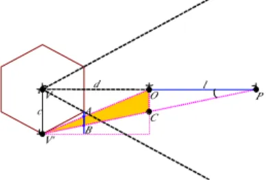
The major problem of depth mesh representation is that it is only the visible part of the object viewed from the cell center hence has limited viewing degree of freedom. When a new view is far from the cell center, parts that are invisible originally might become visible and get rendered as holes. We propose a self-occluding error to estimate the maximum size of the hole that may appear when the object is represented by a depth mesh.
As shown in Figure 1, the maximum error occurs at the farthest view position V’ from the cell center V. Let the cell size, i.e., the length of VV' be c, the distant between object and the cell center, i.e., the length of VO
be d, and the size in depth of the object itself, i.e., the length of OP be l. The length of OC is l*tanθ , the angleθ betweenVP andV 'P is dcl
+ −
= tan 1 θ
and s which is the projected size of OP as well as
OC is: * c AB s = ImageRes. Since , ) ( 2 3 * * 2 2 3 2 3 l d d l c l d cl d c OC d c AB + = + = = therefore, * ) ( 2 3 l d d cl s + = ImageRes.
The test on self-occluding error is to check if the object's maximum projected error s is smaller then a user-specified tolerance in image precision. If it is, the object is represented by a depth mesh; otherwise by a LOD mesh. P c V V' A B O C d l θ
Figur e 1. The maximum self-occluding error occurs at the
position V'.
4.1.4. Dep t h mesh con st r u ct ion
The cached image of an object is obtained by rendering the object using the cell center as the center of projection and using the cell's side face as the projection window.
The depth image is the cached image augmented with the
depth values. The simplest way to construct a depth mesh for an object is to use the regular-grid triangulation6 performed on the depth image, which would, however, results in too many redundant triangles and produces rubber effects caused by incorrect connections. Furthermore, since it is performed in the image space, it always suffers from the precision error caused by the projection (from floating-point precision in world space into integer precision in image space).
In order to reduce the number of the triangles on a depth mesh while preserving most of the visual appearances, several properties of the depth image could be adopted. The most important one is to use the depth coherence, by that we mean pixels of similar depth variation are likely to be on the same surface, and a pixel that has a sharp depth variation from adjacent pixels would have a high possibility to be on a contour edge. Moreover, the external contour edges of the rendered object on the image are the most important visual appearances, and hence must be included in the depth mesh. External contour edges can be easily derived by using the contour extraction in the field of image processing. On the other hand, if we can extract all the internal contour edges from the depth image, rubber effects caused by undetected gaps (C0 discontinuity) between disjointed surfaces represented by a connected mesh and blur effects appearing at the sharp edges (C1
discontinuity) represented by a flatted mesh could be greatly reduced.
In order to minimize the precision error caused by projection, we simplify the depth mesh in both the image and the object space in three steps. Firstly, we categorize image pixels on the depth image based on the importance of its visual appearance and its characteristic into four categories:
l external contour l internal contour (gap) (C0
discontinuity) l sharp edge (C1
discontinuity) l interior
Secondly, vertices of object's original mesh are projected again (but do not alter the value of depth image) with the same projection setup of the depth image to do the visibility test for each vertex. If Z value of a projected vertex equals to the Z value at the pixel on the depth image, the pixel on the depth image is representing
the vertex of the original mesh; otherwise the vertex is behind other surfaces. For the former case, a weight rela-tive to the category of the pixel is assigned to the vertex (The highest weight is assigned for external contour category, a lower weight is assigned for internal contour category, and so on.) On the other hand, for the later case (invisible vertex), the vertex gets zero weight.
Lastly, weight-based edge collapsing is performed based on the weights of vertices to simplify the object's original mesh. Moreover, to obtain a proper resolution of the simplified depth mesh and preserve the visual appearances, the edge with one of or both vertices' weight smaller than the weight of the sharp edge category and whose projected size smaller than a user-specified length tolerance (in pixels) is simplified. The collapsing order is based on the area of the projected triangle. As a result, a more optimized triangle aspect ratio is obtained and tiny triangles with respect to the view contain no important visual appearances are removed.
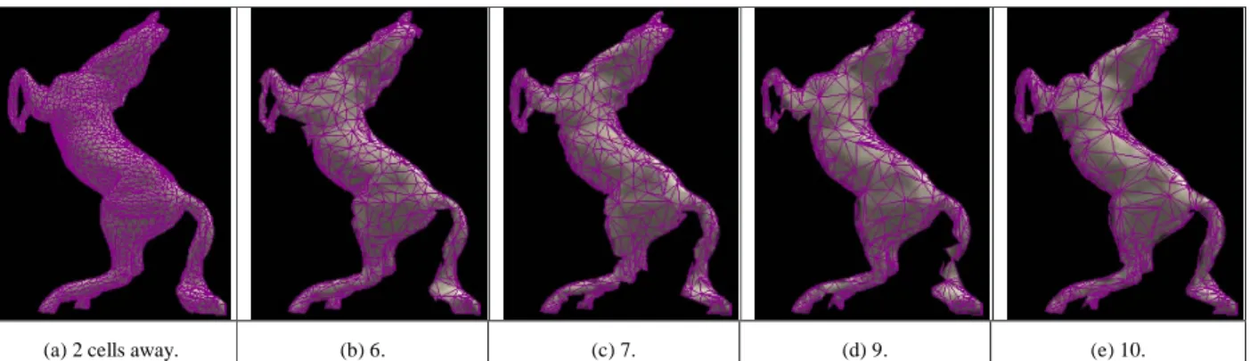
Figure 4(b-e) show the simplified depth meshes at different distances.
4.2. R u n-T ime St a ge
In the run-time stage, we do the following steps:
1. At program start-up time, we setup a lowest priority thread for pre-fetching the geometry and image data of neighboring cells.
2. Ensure that the geometry and image data for the current navigation cell is loaded into memory.
3. Perform a run-time normal-cluster-based back-face culling for the objects inside the current navigation cell.
4. Perform a run-time occlusion culling for all meshes. 5. Render the remaining polygons. Depth meshes are
rendered using the projective-alike texture mapping. 6. Pre-fetch data of neighboring cells when CPU load is
relative low. 4.2.1. R en d er in g
Objects inside the navigation cell can be seen from any direction, it is impossible to determine the visibility during the pre-processing stage. Those polygons inside the navigation cell can be grouped into clusters according to its normal5 in the pre-processing stage. During the run-time stage, we can quickly cull out the whole back-facing cluster of polygons according to the viewing direction and the FOV.
Although there are considerable overheads, it is a beneficial approach to reduce the polygons sent into graphic pipeline by applying a run-time occlusion culling for a densely occluded environment. To perform the
culling, we generate an occlusion map similar to the idea proposed in Ref. 10. Only LOD meshes, depth meshes, and original meshes inside the navigation cell whose projected area larger than a pre-specified threshold are selected to be occluders. Though this approach of occluder selection is not optimized, it is advantageous not to spend too much time on selecting occluders.
5. EXPERIMENTS
Our test scenes are two statuary parks, one is consists of 358 objects with 970,254 polygons (sparse scene), and another is consists of 956 objects with 2,265,978 polygons (dense scene) on an area of 2400×2000.
The test platform is a PC with an AMD TB 1.2Ghz CPU, 512MB main memory, and an nVidia GeForce3 with 64MB DDR RAM graphics accelerator.
5.1. C ell Size a nd Self-O cclud in g E r r or
C onsid er at ion
Several settings of the combination of different cell size (50 and 100) and self-occluding error tolerance (1-, 3-, and 5-pixel) are used in our experimental test.
As we can expect, the higher self-occluding error we can tolerate, the more objects are represented by depth meshes. In the case of cell size 50 and 1-pixel error tolerance, 54.0% objects are represented by depth meshes, while it is 63.9% for 3-pixel error tolerance. However, with no doubt, image quality for 3-pixel tolerance is lower than that of 1-pixel tolerance.
Since we want to identify how much benefit and image quality-loss comes from the depth mesh representation alone, we use original meshes instead of LOD meshes to represent those objects with the self-occluding error exceeding the tolerance. Such that, when cooperating with LOD techniques the performance would be even better.錯誤! 書籤的自我參照不正確。 Table 1 lists the polygon number of regional back-face culled LOD meshes, depth meshes, polygons inside a cell, the number of objects represented by depth mesh, the average frame rate, and average image quality under different settings. Under 60° FOV, three view windows should be rendered, such that, half of the LOD meshes, half of the depth meshes and all meshes inside the cell are the potential visible polygons. All of them show that, more polygons are simplified for the higher error tolerance setting with the cost of higher quality-loss. That is, our proposed scheme provides a tradeoff between the performance and image quality. Note that, under the
Figur e 2. (a) is the original mesh of a horse captured at two cells away (at distance 173), and (b-e) are depth meshes generated at 6, 7, 9
and 10 cells away.
same self-occluding tolerance, a larger cell size would not produce much poorer image quality, mainly due to the fact that the selection of object's representation is designed to ensure the bounded self-occluding error. Hence, the cell size has little impact on the image quality under our proposed scheme. However, as the cell size increases, more objects are represented by LOD meshes, more objects are put inside the navigation cell, and the number of potential visible polygons increases also, so the number of polygons increases dramatically. As a result, worse performance will be found.
The depth mesh simplification can simplify about 94% polygons in average, and, the farther object is, the greater simplification ratio is. On the other hand, in general, the larger size a cell has or the nearer object is, the fewer back-facing rate is. At the time of writing this report, we are still working on several minor bugs of this pre-processing occlusion culling program; therefore, we have no information about how many percentage of polygons could be culled.
5.2. P er for ma n ce
We use the setting of cell size 50 and 3-pixel self-occluding error tolerance for the further testing for the dense scene. Three rendering configurations are used to do the performance comparison:
l A: (Pure geometry) The original meshes of the scene are rendered using the traditional graphics pipeline.
l B: (Pure geometry w/ view frustum culling) Same as A, but with software view frustum culling.
l C: (Pr oposed scheme w/o r un-time occlusion culling)
The scene is rendered by proposed scheme with view frustum culling but without run-time occlusion culling.
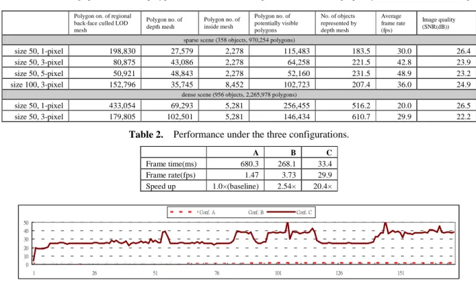
Table 2 lists the performance of each configuration. Configuration C spends additional time on loading
neighboring cell data at the first frame, such that, there is a low peak at the first frame. Our proposed scheme w/o run-time occlusion culling has about 20.4 speedup factor compare to the pure geometric rendering while yields an average SNR about 22.2dB (13.6× under 1-pixel error tolerance and yields an SNR about 26.5dB.) It shows that our proposed method provides a faster rendering with an acceptable quality-loss while configuration B is hardly to achieve interactive frame rate for such complex scene. Figure 3 depicts the frame rate of every rendering frame on the same navigation path under these three rendering configurations.
As mentioned before, the overhead of run-time occlusion culling is un-negligible, and our test scene is not a densely occluded environment, our experiment is, w/ runtime occlusion culling, it is slower than C but still outperforms B.
6. DISCUSSION & FUTURE WORK
In this project, we have proposed a hexagonal spatial subdivision and a hybrid rendering scheme for navigating complex scenes. Such scheme can achieve a smooth, navigation with no apparent popping effects at an almost constant and interactive frame rate for a very complex scene. By cooperating with LOD meshes and object-based depth meshes, parallax error, crack, hole, rubber effect, and popping effect can be minimized. Further-more, with visibility preprocessing, polygons invisible from a region will never be sent into graphics pipeline. A tradeoff between performance and quality requirement can be easily made by specifying the self-occluding error tolerance.
When constructing the depth mesh in both object and image space, a special affair should handle with care.
The rasterization engine of graphics hardware may render small polygon specially, such that a vertex may not projected into the same image pixel, in a result, a wrong weight may retrieved.
As the future works, we will improve the depth mesh construction and simplification to have a better simplified depth mesh. For handling more complicated and extremely large scale scene, distant objects that are close to each other can clustered together to generate a single depth mesh. Such that, the amount of textures could be reduced and an approximated occlusion culling is done on the fly. Moreover, we will try to exploit the data coherence between neighboring cells to improve our pre-loading scheme.
7. REFERENCES
1. S. E. Chen and L. Williams. “View Interpolation for Image Synthesis,” in Computer Graphics (SIGGRAPH 93 Proceedings), pp. 279–288, 1993.
2. L. Darsa, B. Costa, and A. Varshney. “Walkthroughs of Complex Environments using Image-based Simplification,” in Computers & Graphics, volume 22, pp. 55–69, 1998.
3. X. Decoret, G. Schaufler, F. X. Sillion, and J. Dorsey. “Multi-Layered Impostors for Accelerated Rendering,” Computer Graphics Forum, 18(3):61–73, 1999.
4. H. Hoppe, T. DeRose, T. Duchamp, J. McDonald, and W. Stuetzle. “Mesh Optimization,” in Computer Graphics (SIGGRAPH 93 Proceedings), pp. 19–26, 1993.
5. S. Kumar, D. Manocha, B. Garrett, and M. Lin. “Hierarchical Back-face Culling,” In 7th Eurogra-phics Workshop on Rendering, pp. 231–240, 1996.
6. W. R. Mark, L. McMillan, and G. Bishop. “Post-Rendering 3D Warping,” in Symposium on Interactive 3D Graphics, pp. 7–16, 1997.
7. L. McMillan and G. Bishop. “Plenoptic Modeling: An Image-Based Rendering System,” in Proceedings of SIGGRAPH 95, pp. 39–46, 1995.
8. J. Shade, D. Lischinski, D. H. Salesin, T. DeRose, and J. Snyder. “Hierarchical Image Caching for Accelerated Walkthroughs of Complex Environments,” in Proceedings of SIGGRAPH 96, pp. 75–82, 1996. 9. F. Sillion, G. Drettakis, and B. Bodelet. “Efficient
Impostor Manipulation for Real-Time Visualization of Urban Scenery,” in Proceedings of Eurographics’97, pp. 207–218, 1997.
10. H. Zhang, D. Manocha, T. Hudson, and K. Hoff. “Visibility Culling Using Hierarchical Occlusion Maps,” in Computer Graphics, volume 31, pp. 77–88, 1997.
Table 1. The average potential visible polygon no. for a cell, the average frame rate, and image quality under the different settings.
Polygon on. of regional back-face culled LOD mesh Polygon no. of depth mesh Polygon no. of inside mesh Polygon no. of potentially visible polygons No. of objects represented by depth mesh Average frame rate (fps) Image quality (SNR(dB)) sparse scene (358 objects, 970,254 polygons)
size 50, 1-pixel 198,830 27,579 2,278 115,483 183.5 30.0 26.4 size 50, 3-pixel 80,875 43,086 2,278 64,258 221.5 42.8 23.9 size 50, 5-pixel 50,921 48,843 2,278 52,160 231.5 48.9 23.2 size 100, 3-pixel 152,796 35,745 8,452 102,723 207.4 36.0 24.9
dense scene (956 objects, 2,265,978 polygons)
size 50, 1-pixel 433,054 69,293 5,281 256,455 516.2 20.0 26.5 size 50, 3-pixel 179,805 102,501 5,281 146,434 610.7 29.9 22.2
Table 2. Performance under the three configurations.
A B C Frame time(ms) 680.3 268.1 33.4 Frame rate(fps) 1.47 3.73 29.9 Speed up 1.0×(baseline) 2.54× 20.4× 0 10 20 30 40 50 1 26 51 76 101 126 151
Conf. A Conf. B Conf. C