非線性不確定系統模糊類神經網路控制器的硬體實作

全文

(1)國立交通大學電機與控制工程研究所碩士論文非線性不確定系統模糊類神經網路控制器的硬體實作 Real-Time Hardware Implementation of Intelligent Adaptive Fuzzy Neural Network Controller For Uncertain Nonlinear Systems. 研究生：林晏暘指導教授：王啟旭. 中華民國九十四年六月.

(2) 非線性不確定系統模糊類神經網路控制器的硬體實作學生：林晏暘. 指導教授：王啟旭教授. 國立交通大學電機與控制學系. 摘要本篇論文中，以 TS 形式的模糊類神經網路模型為基礎的即時智慧型適應控制方法，用硬體實作出來，控制行星倒單擺系統。這個硬體平臺是 dSPACE DS 1104 R&D control board，可以搭配 MatLab 在 Windows 2000 下運作。在模擬與實作上都獲得很好的結果。並且經由模擬與實作，探討了運算的時間延遲對這個控制器效能的影響。從實作探討出來的運算時間延遲來看，我們可以使用更經濟的硬體平台來實踐這個控制方法，應用到工業上。. I.

(3) Real-Time Hardware Implementation of Intelligent Adaptive Fuzzy Neural Network Controller For Uncertain Nonlinear Systems Student: 林晏暘. Adviser: 王啟旭教授. Department of Electrical and Control Engineering National Chiao Tung University. Abstract In the thesis, true hardware implementation of an on-line intelligent adaptive TSK FNN controller is performed to control the planetary inverted pendulum. The hardware platform is dSPACE DS 1104 R&D control board under Windows 2000 running with MatLab. Excellent agreements have been obtained between theoretical simulation and hardware implementation. The effects of computational time delay for controller is also investigated through both software simulation and hardware emulation and by building SimuLink blocks in MatLab. The estimated maximum computational time delay can be quite practical for the industrial applications to choose cheaper hardware platform with less cost.. II.

(4) 誌. 謝. 兩年的研究所學業，最後用這一本小小的論文作為結束，感謝所有口試委員的指教。在這兩年的時光，感謝家人給我的支持，感謝指導教授王啟旭老師的指導，感謝我的每一位朋友，在每一刻最需你們的時候，總是不吝給予協助，謝謝。. III.

(5) 摘要. I. ABSTRACT. II. 誌謝. III. CONTENTS. IV. LIST OF FIGURES. V. LIST OF TABLES. VI. CONTENTS Chapter 1 Introduction. 1. Chapter 2 Theoretical Foundation. 3. 2.1. TS-Type FNN Model for Uncertain Systems. 3. 2.2. On-Line Optimal Training. 5. 2.3. Design Algorithm for Computer Simulation. 7. 2.4. Simulation with Computational Time Delay. 11. Chapter 3 Real-Time Control of Planetary Inverted Pendulum. 15. 3.1. Planetary Inverted Pendulum. 15. 3.2. Simulation. 17. 3.3. Simulation with Computational Time Delay. 21. 3.4. Hardware Implementation. 24. I.. Hardware platform DS 1104 R&D control board. 24. II.. Design flow. 25. III. Building the control block. 27. Chapter 4 Conclusion. 35. Reference. 36. IV.

(6) LIST OF FIGURES Figure 2-1.. TS-type FNN model for Uncertain Systems. 4. Figure 2-2.. Overall design process. 7. Figure 2-3.. Block diagram of mass-spring-damper system. 9. Figure 2-4.. Block diagram of “Trained TK-Model” in Figure 2-3. 9. Figure 2-5.. Training block in Figure 2-4. 10. Figure 2-6.. Block diagram of “Design Controller” in Figure 2-3. 10. Figure 2-7.. Trajectories for x1 and x2 in Example 1. 11. Figure 2-8.. Mass-spring-damper system with time delay. 12. Figure 2-9.. Time response of Example 1 with delay time = 0.35s. 13. Figure 2-10. Time response of Example 1 with delay time = 0.37s. 13. Figure 2-11. Time response of Example 1 with delay time = 0.39s. 14. Figure 3-1.. Planetary inverted pendulum. 15. Figure 3-2.. The fixed-star gear and the planetary gear. 16. Figure 3-3.. MF of θ&0 (rad/s). 18. Figure 3-4.. MF of θ0. 18. Figure 3-5.. Simulation model of the planetary inverted pendulum system. 19. Figure 3-6.. Block diagram of “Trained TK-Model” in Figure 3-5. 20. Figure 3-7.. Block diagram of “Design Controller” in Figure 3-5. 20. Figure 3-8.. Trajectories for θ0 in Figure 3-5. 21. Figure 3-9.. The inverted pendulum system with time delay. 22. (rad). Figure 3-10. Trajectories of θ0 with delay time = 0.015s in Figure 3-9. 22. Figure 3-11. Trajectories of θ0 with delay time = 0.022s in Figure 3-9. 23. Figure 3-12. Trajectories of θ0 with delay time = 0.023s in Figure 3-9. 23. Figure 3-13. Overall hardware configuration using DS 1104. 24. Figure 3-14. MF of θ&0 (rad/s). 25. Figure 3-15. MF of θ0. 26. (rad). Figure 3-16. The dSPACE control block diagram for inverted pendulum. 27 V.

(7) Figure 3-17. Block diagram of “Select output timing” in Figure 3-16. 27. Figure 3-18. Trajectory of θ0 for flinging pendulum upward in Figure 3-16. 28. Figure 3-19. Block diagram of “FNN controller” in Figure 3-16. 28. Figure 3-20. Block diagram of “Trained TK-Model” in Figure 3-19. 29. Figure 3-21. Block diagram of “Design Controller” in Figure 3-19. 29. Figure 3-22. Trajectory for θ0 in Figure 3-16. 30. Figure 3-23. Trajectory of θ0 during the stabilization of the pendulum in. 30. Figure 3-22 Figure 3-24. Trajectory of θ0 during the stabilization of the pendulum with the. 31. application of the control method as θ0<15° Figure 3-25. The dSPACE inverted pendulum control block diagram with. 31. “Integer Delay” block Figure 3-26. Trajectory of θ0 to stabilize the pendulum with time delay =. 32. 0.014s Figure 3-27. Trajectory of θ0 to stabilize the pendulum with time delay =. 33. 0.019s Figure 3-28. Trajectory of θ0 to stabilize the pendulum with time delay =. 33. 0.020s. LIST OF TABLES Table 3.1.. Four nominal operating points with initial weighting matrices. 18. Table 3.2.. Four nominal operating points with initial weighting matrices. 26. VI.

(8) CHAPTER 1 Introduction When we want to control a system, it usually has to be identified to have a mathematical model. But, in fact, it is often difficult to get the mathematical model, because the mathematical models of most systems are complex. Fuzzy neural network such as Takagi-Sugeno(TS)-Type FNN Model can simplify the process of identification of a system, and then the identified model can be controlled by the control technique. An on-line intelligent adaptive control was proposed in [1], which uses optimally trained TS-type FNN model [2] to identify an uncertain nonlinear system and then designs the controller with pole placement technique. Theoretically, applying the approach can obtain the TS-type FNN model of an uncertain nonlinear system in real-time environment and get a good controller to achieve the control specifications. The results of simulating some examples in [1] are good. But, it needs a large amount of computation to accomplish the training model, even though the optimal training [3] and the least square initialization [4] have shortened the process of training. In the implementation, computational delay will be an important factor in time delay. For example, in comparison with the PID control method, it is easy to design controller using on-line intelligent adaptive control with TS-type FNN models. For a PID control system, the transfer function has to be found [11]. It is usually difficult to find the transfer function of an uncertain nonlinear system. The theme of the thesis is to implement a controller to control a system with on-line intelligent adaptive control for uncertain nonlinear system using TS-type FNN models. The planetary inverted pendulum [7] will be controlled within the hardware platform, DS 1104 R&D control board. As the excellent results of some examples presented in the thesis [1], our simulation for the planetary inverted pendulum controlled by the on-line intelligent adaptive control approach is fine, too. For implementation of the on-line optimal training controller, the design of on-line training process and the estimation for initial matrices for TS-type FNN model are the two major problems. The first one is how to train TS-type FNN model on-line. We use the “memory” and “pulse generator” blocks to build a training block to achieve the on-line training. We can determine the re-training time instant by setting the “pulse generator” block. For the second problem, it will be explained in the real-control in chapter 3. Page 1.

(9) There are three parts in the thesis: I.. Introduction to the on-line adaptive intelligent control for uncertain nonlinear system using TS-type FNN model. II. Real-time control of planetary inverted pendulum III. Conclusion Part I consisting of Chapter 2 includes the identification of an uncertain nonlinear system with TS-type FNN model and the application of pole placement technique in design of the controller. For the training of TS-type fuzzy model, dynamic optimal training [3] is used to guarantee the fastest convergence of the training process. And we applied least square estimation-technique [4] to estimate the initial weighting matrices for TS-type FNN model. The proper initial weighting number can guarantee the convergence. The simulation of the mass-spring-damper control system using this control approach is involved in the part. We make the output of the nonlinear uncertain control system to track a sinusoidal signal. Part II consisting of Chapter 3 presents the real-time control of planetary inverted pendulum. We introduce the planetary inverted pendulum [7] and the hardware platform, DS 1104 R&D control board [7] [8]. We present the simulation for the planetary inverted pendulum system in SimuLink and then implement the on-line optimal training controller to control the inverted pendulum in the dSPACE system. The time delay for the planetary inverted pendulum system is studied. Finally, in Part III, we give a conclusion.. Page 2.

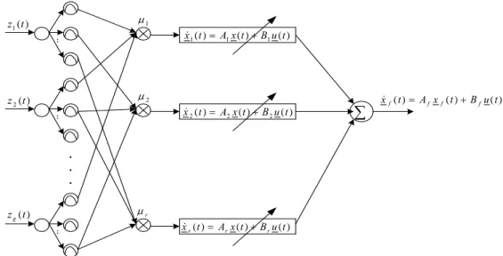
(10) CHAPTER 2 Theoretical Foundation In this chapter, on-line intelligent adaptive control for uncertain nonlinear systems by using optimally trained TS-type FNN models [1] will be reviewed first. The SimuLink simulation of mass-spring-damper system with the design algorithm proposed in [1] will be presented first. The computational time delay, or the control input delay, will also be simulated in this example.. 2.1 TS-Type FNN Model for Uncertain Systems A system can be represented by the following rules of TS-type FNN model [2], where Fij is the FNN set.. Rule 1: If z1 ( t ) is F1,1 and . . . and z g ( t ) is F1, g then x&1 (t ) = A1 x1 (t ) + B1 u (t ) M. (1). M. Rule r: If z1 ( t ) is Fr ,1 and . . . and z g ( t ) is Fr , g then x& r (t ) = Ar x r (t ) + Br u (t ) The above FNN system should be inferred as [1]: r. x& f (t ) = ∑ µ i ( z (t ))[ Ai x f (t ) + Bi u(t )] = A f x f (t ) + B f u(t ). (2). i =1. where z (t ) = [ z1 (t ). z 2 (t ) .... z g (t )]T. g. ∏F. ij. µ i ( z (t )) =. j =1. r. g. i =1. j =1. ∑ (∏ F ). Î. r. ∑ µ ( z (t )) = 1 i =1. i. (3). ij. and r is the number of rules for the uncertain nonlinear systems. Equation (2) shows that the system can be represented by a linear dynamical equation at any time instant, which can be inferred from the TS-type FNN model. Page 3.

(11) The following Figure 2-1 shows the TS-type FNN model explained above. µ1. z1 (t ). x& 1 ( t ) = A1 x ( t ) + B1 u ( t ). :. µ2. z 2 (t ). x& 2 ( t ) = A2 x ( t ) + B 2 u ( t ). :. ∑. x& f ( t ) = A f x f ( t ) + B f u ( t ). . . .. µr. z g (t ) :. x& r ( t ) = Ar x ( t ) + B r u ( t ). Figure 2-1. TS-type FNN model for Uncertain Systems. In Fig. 2-1, z1 (t ) , z 2 (t ) , . . . , z g (t ) are the premise variables and r is the number. of if-then rules and the Ai and Bi matrices are the locally linearized well-specified systems. The Ai and Bi matrices in Fig. 1 are called Jacobian matrices [1] with x&% i (t ) = Ai x% (t ) + Bi u% (t ). (4). In the on-line intelligent adaptive control method in [1], the TS-type FNN model will be trained, so that the matrices Ai and Bi will be different at different time instants. Furthermore if better initial Ai and Bi matrices are chosen, it can take less time to converge. Hence, the least square estimation-technique [4] is chosen to estimate the initial value of the Ai and Bi [1]. Assume the order of the linear subsystems of TS-type FNN model is n and the number of input is m, then we must measure n+m outputs to get the estimated initial matrices [1]. ⎡ AT ⎤ Wi ( 0 ) = ⎢ iT ⎥ ⎣ Bi ⎦ Y = θWi ( 0 ) + ε. (5). Wi ( 0 ) = (θ T θ ) −1θ T Y Where the ε is the noise matrix, and θ and the set of outputs Y are presented as follows.. Page 4.

(12) ⎡ x 1T u 1T ⎤ ⎢ T ⎥ T x u2 ⎥ θ =⎢ 2 ⎢ ⎥ : ⎢ T ⎥ T ⎣⎢ x n + m u m + n ⎦⎥. (6). ⎡ x& 1T ⎤ ⎢ T ⎥ x& Y =⎢ 2 ⎥ ⎢ : ⎥ ⎢ T ⎥ ⎢⎣ x& n + m ⎥⎦. (7). 2.2 On-Line Optimal Training The TS-type FNN model for uncertain systems can be trained by using the on-line optimal training [1]. Because the dynamic optimal training [3] is very powerful for on-line disturbance rejection, it will be utilized in the on-line optimal training of TS-type FNN model for uncertain nonlinear systems. Let the input training matrix R be R = [ x1 (t ) x 2 (t ) ... x n (t ) u1 (t ) ... u 2 (t )]T ∈ ℜ ( m + n )×1. (8). And the output matrix of the TS-type FNN model is Y = x& f (t ) = [ x& f1 (t ) x& f 2 (t ) ... x& f n (t )]T ∈ ℜ n×1. (9). And the output matrix of the uncertain nonlinear system is D = x& (t ) = [ x&1 (t ) x& 2 (t ) ... x& n (t )] ∈ ℜ1xn. (10). The overall weighting matrix to include the uncertain Ai and Bi matrices can be shown as [1]: ⎡ r T⎤ ⎢∑ µ i Ai ⎥ r W = ⎢ i =r1 ⎥ = ∑ µ iWi ⎢ µ B T ⎥ i =1 i i ⎢⎣∑ ⎥⎦ i =1. and. ⎡ AiT ⎤ Wi = ⎢ T ⎥ ⎣ Bi ⎦. (11). Therefore the output of TS-type FNN model Y can be shown as:. Y = RTW. (12). It is therefore the purpose of on-line training to obtain the weighting matrix W . Page 5.

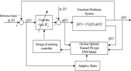
(13) First, the squared error J and the error function E have to be defined:. J =. 1 || x& f − x& ||2 2mn. (13). E = x& f (t ) − x& (t ) = R T W − D. (14). From (13) and (14), we can have J =. 1 Tr( EE T ) 2mn. (15). Then the dynamical learning rates βopt for each iteration k can be determined by the dynamical optimal training in [3]. Define J k +1 − J k = aβ 2 + bβ. (16). where a=. [. ]. 1 (mn) −3 Tr R T RE k E kT R T R > 0 2. [. ]. b = −(mn) −2 Tr E kT R T RE k < 0. (17) (18). The roots of aβ2 + bβ = 0 are (βu ,βl). The optimal learning rate βopt will be βopt = (βu+βl)/2 = βt (19) This learning rate will not only guarantee the stability of the training process, but also have the fastest speed of convergence. Then, the on-line training rule for each subsystem is shown as Wi (k + 1) = Wi (k ) − β opt ,k. 1 REk mn. (20). The Ai and Bi matrices for each subsystem of TS-type FNN model can be updated simultaneously by using (20) at the beginning of each time interval. The final linear dynamic equation, (Af, Bf), of the uncertain nonlinear system has been inferred from (2) at the beginning of any time interval. Then, the pole placement technique can be used to design the controller [1]. The overall design process can be seen from the following Figure 2-2, which is from [1].. Page 6.

(14) u s (t) Reference Input. ur (t). −. ε (t). +. Controller Gain K p. + −. u(t). Uncertain Nonlinear System. x(t). x&(t) = f (x(t), u(t)) x&(t). Design of tracking controller. On-line Optimal Trained TS-type FNN Model. Adaptive Rules. Figure 2-2. Overall design process. 2.3 Design Algorithm for Computer Simulation If we ignore the inevitable computational time delay, which includes the training time, the pole-placement and signal transmission, a design algorithm from [1], which is based on Figure 2-2, can be summarized as follows: Step (1) Step (2). Specify desired stable poles. Define the r nominal operating points and the corresponding membership functions for x(t ) and x& (t ) . Use any input u(t) to excite the uncertain nonlinear system and measure sufficient data information of x(t ) and x& (t ) . In real implementation, it is easier to use step commands to trigger the system to get sufficient response data. This will be explained later in the real–time control of planetary inverted pendulum in Chapter 3. Apply (5) to find the initial weighting matrix Wi (0 ) of each subsystem for. i=1, …, r. Step (3) Apply pole placement to design the controller. Step (4) If the norm of tracking error > e1, a specified threshold, GOTO Step (2), Else GOTO Step (5). Step (5) Measure on-line x(t ) and x& (t ) . For i=1,…, r, applying (19) to find the optimal. learning rates to train the weighting matrix of each subsystem. The optimal training must continue until relative errors of Wi are less than another pre-defined threshold e2. Step (6) GOTO Step (3). Page 7.

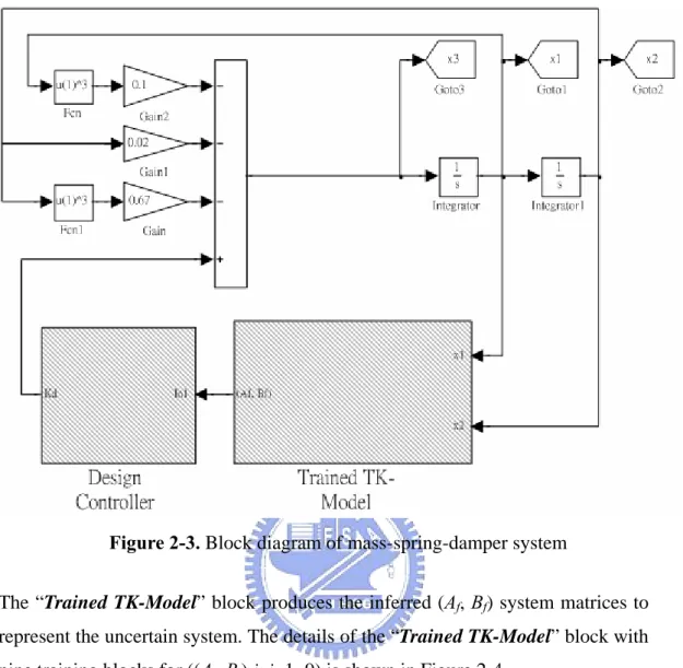
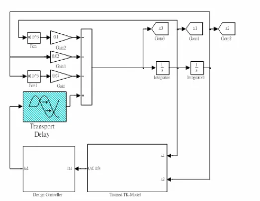
(15) Adaptive Rules for updating the closed-loop system in Figure 2-2. If || ε (t ) ||> Threshold Apply all Steps to update the TS-type FNN model, us(t) and Kp Else Stand Still End. The above design algorithm can be best illustrated by the following example.. Example 1. The Mass-Spring-Damper System Consider the mass-spring-damper system [1] of which the mathematical equation is &x& = −0.1x& 3 − 0.02 x − 0.67 x 3 + u and let [ x(t ) x& (t ) ]r = [ x2. x1 ] . In this example,. the objective of the control system is to make the position, x2 , and the velocity, x1 , trace the reference signal. Now, follow the design flow and rule to implement the controller. Step (1) Specify the closed-loop poles as -2 and -1.5 Step (2) According to the distribution of the output signal, define the membership function. Then, use the equation (5) to estimate the initial value. Step (3) Design the controller (Figure 2-6). Step (4) Apply Adaptive Rules to update the TS-type FNN model and the controller to stabilize the closed-loop system.. We run the simulation of the above system using SimuLink with on-line optimal training and controller design. SimuLink is a graphic extension of MATLAB for modeling and simulation of systems. Figure 2-3 shows the overall SimuLink blocks for the mass-spring-damper system. The “Trained TK-Model” (which includes model description and on-line optimal training) and “Design Controller” blocks are placed in Figure 2-3.. Page 8.

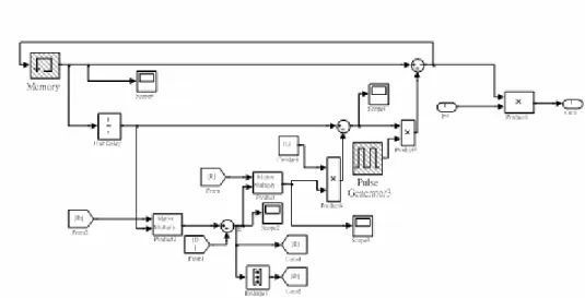
(16) Figure 2-3. Block diagram of mass-spring-damper system. The “Trained TK-Model” block produces the inferred (Af, Bf) system matrices to represent the uncertain system. The details of the “Trained TK-Model” block with nine training blocks for ((Ai, Bi) i, i=1~9) is shown in Figure 2-4.. Figure 2-4. Block diagram of “Trained TK-Model” in Figure 2-3. Figure 2-5 shows the details of the training block in Figure 2-4. The objective of Page 9.

(17) the “Memory” block in Figure 2-5 is to memorize the training results from previous training and the “Pulse Generator” block is to set the training time interval.. Figure 2-5. Training block in Figure 2-4.. Figure 2-6. Block diagram of “Design Controller” in Figure 2-3. The details of “Design Controller” block in Figure 2-3 can be seen from Figure Page 10.

(18) 2-6. After the training process, the “Design Controller” block collects the system’s mathematical model and applies pole placement technique to design the controller.. In conclusion, the on-line intelligent adaptive control involves two steps: 1. 2. The. [ x1. System identification using on-line optimal training Design of controller using pole-placement technique. simulation. results. are. shown. in. Figure. 2-7. with. initial. state,. x2 ] = [ 0.2 0.2] .. Figure 2-7. Trajectories for x1 and x2 in Example 1. 2.4 Simulation with Computational Time Delay In real life, the system has the inevitable time delay associated with it, which includes the training time, the pole-placement and signal transmission [10]. Time delay often occurs in electronic, mechanical, chemical, etc., systems. They may be due to some Page 11.

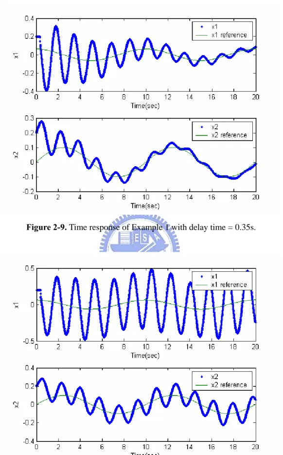
(19) the following causes: 1. Measurement of system variable. 2. Physical properties of the equipment used in the system. 3. Signal transmission. 4. Computational delay. The effect of time delay depends on the size of the delay and the system characteristics. In Example 1, it will need a lot of time to train the TS-type model and to design the controller. To understand the effects of real time-delay on the real system, a “Transport Delay” block is added to Figure 2-3, which is shown in Figure 2-8. The “Transport Delay” block enumerates the time delay associated with “Trained TK-Model” and “Controller Design”. Figure 2-9 and 2-10 show the responses of Example 1 with time delay = 0.35s and 0.37s respectively. It is obvious that the longer is the delay time, the more oscillatory the response will be.. Figure 2-8. Mass-spring-damper system with time delay. Page 12.

(20) Figure 2-9. Time response of Example 1 with delay time = 0.35s.. Figure 2-10. Time response of Example 1 with delay time = 0.37s.. Page 13.

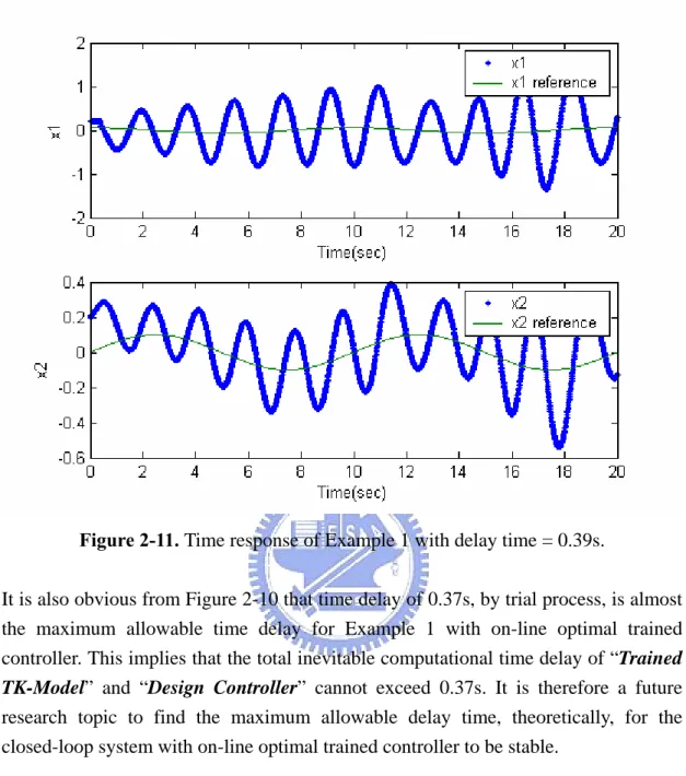
(21) Figure 2-11. Time response of Example 1 with delay time = 0.39s.. It is also obvious from Figure 2-10 that time delay of 0.37s, by trial process, is almost the maximum allowable time delay for Example 1 with on-line optimal trained controller. This implies that the total inevitable computational time delay of “Trained TK-Model” and “Design Controller” cannot exceed 0.37s. It is therefore a future research topic to find the maximum allowable delay time, theoretically, for the closed-loop system with on-line optimal trained controller to be stable.. Page 14.

(22) CHAPTER 3 Real-Time Control of Planetary Inverted Pendulum In the preceding chapter, we have reviewed the on-line intelligent adaptive control for uncertain nonlinear systems by using optimally trained TS-type FNN models. We have also presented the SimuLink simulation for the mass-spring-damper system with the design algorithm in [1]. In this chapter, we will employ the same methodology to design the planetary inverted pendulum control system. According to the design flow, we will estimate the initial weighting matrices and then train the model and design the on-line controller. The amount of computation of training the TS-type FNN model is large, so the incurred computational time delay will influence the performance of the controller. In the following, there are four parts in the chapter: I.. Introduction to the planetary inverted pendulum. II.. Simulation without computational delay. III. Simulation with time delay IV. Hardware implementation. 3.1 Planetary Inverted Pendulum The planetary inverted pendulum [7] is shown in Figure 3-1. A PID controller was designed to control the system in [7]. In this chapter, the control approach, on-line intelligent adaptive control for uncertain nonlinear systems using optimally trained TS-type FNN models, is applied to control the planetary inverted pendulum system.. Figure 3-1. Planetary inverted pendulum.. Page 15.

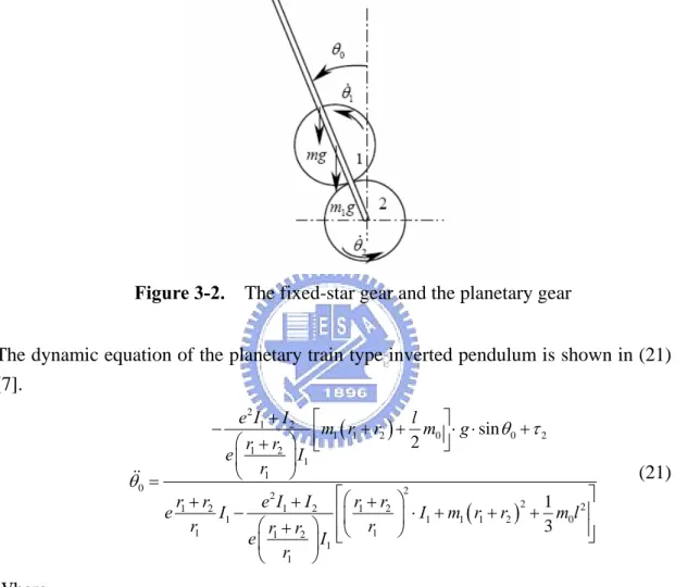
(23) From Figure 3-1, electric motor 29 drives the fixed-star gear, gear 9, to give it an angular acceleration. Then gear 9 drives gear 3, the planetary gear, so that gear 3 would orbit gear 9. We use a bearing and shaft 2 to fix gear 3 with pendulum 1 so that pendulum 1 will orbit gear 9. Therefore, pendulum 1 is drove by electric motor 29, and the angular position of pendulum 1 can be detected by sensor 30. Figure 3-2 shows the coupling of gear 1 and gear 2, which steers pendulum 1.. Figure 3-2. The fixed-star gear and the planetary gear. The dynamic equation of the planetary train type inverted pendulum is shown in (21) [7]. −. θ&&0 =. e2 I1 + I 2 ⎡ l ⎤ m1 ( r1 + r2 ) + m0 ⎥ ⋅ g ⋅ sin θ 0 + τ 2 ⎢ 2 ⎦ ⎛r +r ⎞ ⎣ e ⎜ 1 2 ⎟ I1 ⎝ r1 ⎠. (21). ⎤ r1 + r2 e2 I1 + I 2 ⎡⎛ r1 + r2 ⎞ 1 2 2 ⎢⎜ I1 − ⎟ ⋅ I1 + m1 ( r1 + r2 ) + m0l ⎥ r1 3 ⎛r +r ⎞ ⎢ r ⎥⎦ e ⎜ 1 2 ⎟ I1 ⎣⎝ 1 ⎠ ⎝ r1 ⎠ 2. e. Where. τ 0 : Torque of driving the pendulum τ 2 : Torque of electric motor driving the fixed - star gear θ、 2 θ、 1 θ 0 : The angle of the fixed - star gear , the planetary gear and the pendulum with respect to vertical N、 1 N 2 : The number of teeth of the planetary gear and the fixed - star gear m、 2 m、 1 m0 : The mass of the fixed - star gear , the planetary gear and the pendulum I、 1 I 2 : The moment of inertia of the planetary gear and the fixed - star gear r、 1 r2 : The radius of the planetary gear and the fixed - star gear l : The dis tan ce of the pendulum r e=− 2 r1 Page 16.

(24) 3.2 Simulation Before the hardware implementation of the controller for the planetary inverted pendulum system, we perform the simulation for the inverted pendulum system in SimuLink. The control objective of this control system is to stabilize the inverted pendulum after the pendulum has been flung upward. The process includes two stages [7]: 1. Flinging the pendulum upward 2. Stabilization of the pendulum in the upward direction In the first stage, we give a small torque to make the pendulum oscillate slightly and then control the electric motor’s output according to the oscillation frequency of the pendulum to enlarge the pendulum’s swing amplitude. When θ0 is smaller than 10°, the second stage begins. In the second stage, we apply on-line intelligent adaptive control with the optimally trained TS-type FNN model to stabilize the inverted pendulum system in dynamic equilibrium point (θ0=0). The control method is applied in the second stage, so we will run the simulation for the second stage with the initial condition, θ&0 =1(rad/s) and θ 0 =0.17(rad). The following parameters are assumed in [7], which will be applied in (21): m1 , m2 : 0.08kg m0 : 0.08kg r1 , r2 : 0.013m l : 0.12m I1 , I 2 : 6.76e − 6 kg − m 2 e : −1 Thus, we have the dynamical equation:. θ&&0 = 149.3003sin θ 0 + 2214.3u. (22). Step (1) Specify the closed-loop poles as -2 and -1.5 Step (2) The mathematical equation of the inverted pendulum system has been described in (22). We apply u=0.03sin (t) to the inverted pendulum system for measurements of θ& ( t ) and θ&& (t ) . According to the distribution of the 0. 0. measured data, the membership functions for θ&0 and θ 0 can be defined as the follows:. Page 17.

(25) Figure 3-3. MF of θ&0 (rad/s). Figure 3-4. MF of θ 0 (rad) The order of the TS-type FNN model for the inverted pendulum system is two and the number of input is one, so we measure three outputs to get the estimated initial value. We choose four nominal operating points, i.e., r=4. The nominal operating points and the initial weighting matrices are shown in the Table 3-1. Table 3-1. Four nominal operating points with initial weighting matrices R. 1. [ θ&0 θ 0 ]. [ -2 , -0.17 ]. ⎡ ArT ⎤ Wr = ⎢ T ⎥ ⎣ Br ⎦. 0. 0. 1.0e+003 * ⎡ -0.0002 0.0010 ⎤ ⎢ 0.0873 0 ⎥⎥ ⎢ ⎢⎣ 2.2139 0 ⎥⎦. Page 18.

(26) 2. 3. 4. [ -2 , 0.17 ]. 1.0e+003 * ⎡ 0.0002 0.0010 ⎤ ⎢ 0.0873 0 ⎥⎥ ⎢ ⎢⎣ 2.2144 0 ⎥⎦. [ 2 , -0.17 ]. 1.0e+003 * ⎡ 0.0007 0.0010 ⎤ ⎢ 0.0879 0 ⎥⎥ ⎢ ⎢⎣ 2.2113 0 ⎥⎦. [ 2 , 0.17 ]. 1.0e+003 * ⎡ 0.0001 0.0010 ⎤ ⎢ 0.0870 0 ⎥⎥ ⎢ ⎢⎣ 2.2145 0 ⎥⎦. Step (3): Design controller with pole placement technique for the closed-loop poles as -2 and -1.5. Step (4): Apply Adaptive Rules to update the TS-type FNN model and the controller to stabilize the closed-loop system. The control system model and the controller are shown in Figures 3-5~3-7. Figure 3-8 illustrates the trajectory for θ 0 with the initial condition ⎡⎣θ&0 θ 0 ⎤⎦ = [ −2 0.17 ] .. Figure 3-5. Simulation model of the planetary inverted pendulum system. Page 19.

(27) Figure 3-6. Block diagram of “Trained TK-Model” in Figure 3-5. Figure 3-7. Block diagram of “Design Controller” in Figure 3-5. Page 20.

(28) Figure 3-8. Trajectories for θ 0 in Figure 3-5. 3.3 Simulation with Computational Time Delay In this section, we consider the effect of time delay on the angular control system of planetary inverted pendulum. We add the “Transport Delay” block into the Figure 3-5, which is shown in Figure 3-9. Figure 3-10 and 3-11 show the responses of the control system with time delay = 0.015s and 0.022s respectively. We can find that θ& and 0. θ 0 are always oscillatory and the longer is the delay time, the more oscillatory the responses will be. From Figure 3-11, the time delay of 0.022s is almost the maximum time delay for the inverted pendulum system with the on-line optimal trained controller.. Page 21.

(29) Figure 3-9. The inverted pendulum system with time delay. Figure 3-10. Trajectories of θ 0 with delay time = 0.015s in Figure 3-9. Page 22.

(30) Figure 3-11. Trajectories of θ 0 with delay time = 0.022s in Figure 3-9. Figure 3-12. Trajectories of θ 0 with delay time = 0.023s in Figure 3-9. Page 23.

(31) 3.4 Hardware Implementation I. Hardware platform DS 1104 R&D control board We will implement a controller to control this uncertain nonlinear system by using on-line intelligent optimally adaptive control method. In the beginning, we design the controller in SimuLink and generate the control program and then sent it into the hardware platform, DS 1104 R&D control board, to control the inverted pendulum system. The overall control process is shown in Figure 3-13.. Figure 3-13. Overall hardware configuration using DS 1104 SimuLink is an interactive environment for modeling an off-line simulation with easy-to-use diagram. In MATLAB, Real-Time Workshop can automatically generate C code from SimuLink block diagrams. Together with dSPACE’s Real-Time Interface, these tools can transfer the C code generated from our block diagram to dSPACE’s Real-Time hardware. Here, DS 1104 R&D Controller Board is selected. dSPACE system is the platform for electronic control unit (ECU) development. It provides the V-cycle concept in the development process, in which control design is involved. In dSPACE system, control design is model-based so that we can work with a single model of a complete system in an integrated software environment, as SimuLink. dSPACE hardware includes a powerful processor and numerous I/O interfaces. The processor can calculate our models in real time, and these I/O interfaces can connect to outside world. The hardware, DS 1104 R&D Controller Board, can run directly in the PC. For the implementation of the controller for the planetary inverted pendulum system, we build the control block in SimuLink and generate the C code, and then sent the C code into the dSPACE hardware. We will operate the hardware to control the Page 24.

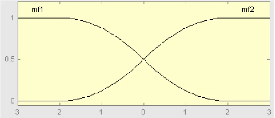
(32) planetary inverted pendulum through the dSPACE system interface.. II. Design flow We have presented the simulation for the inverted pendulum system via the on-line intelligent adaptive control approach. The control block for the planetary inverted pendulum system has been built in SimuLink. But, from (22), the input of the system is torque. In the real planetary inverted pendulum system, the input is voltage. The mathematical relation between torque and voltage is unknown, so that the mathematical relation between the voltage and the angle of inverted pendulum is uncertain and nonlinear. Step (1) Specify the closed-loop poles as -2 and -1.5. Step (2) Define the membership function and estimate the initial weighting matrices. Because the order of the TS-type FNN model is two and the number of input is one, we have to measure three outputs to estimate the initial matrices. The controller is applied in the second stage, so we have to get the estimated initial matrices when θ0 is between 10° and -10°. But, when θ0 is between 10° and -10°, it is difficult to apply u = 10sin (t) to the inverted pendulum system to measure θ&0 and θ&&0 . Therefore we apply three step commands (u = 10 volts) as the inputs to the system to get sufficient data ( θ&0 and θ&&0 ) to estimate the initial matrices with least square estimation-technique. For this uncertain nonlinear system, when θ0 equals to 10°(= 0.1745rad), 15°(= 0.2018rad),. 20°(= 0.3491rad) respectively, we. apply u = ±10V to electric motor 29 to drive the pendulum for measurements of θ&0 and θ&&0 . The membership functions for θ&0 and θ0 can be defined as the follows:. Figure 3-14. MF of θ&0 (rad/s) Page 25.

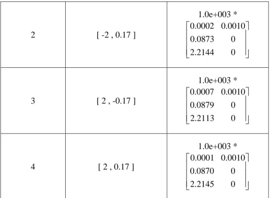
(33) Figure 3-15. MF of θ 0 (rad) There are four nominal operating points. The nominal operating points and the initial weighting matrices are shown in the Table 3-2.. Table 3-2. Four nominal operating points with initial weighting matrices R. 1. 2. 3. 4. [ θ&0 θ 0 ]. ⎡ AT ⎤ Wr = ⎢ rT ⎥ ⎣ Br ⎦. 0. 0. [ -2 , -0.2 ]. ⎡ −0.9817 1 ⎤ ⎢103.1952 0 ⎥ ⎢ ⎥ ⎢⎣ −3.1467 0 ⎥⎦. [ -2 , 0.2 ]. ⎡ 0.4661 1 ⎤ ⎢152.4319 0 ⎥ ⎢ ⎥ ⎢⎣ 2.2814 0 ⎥⎦. [ 2 , -0.2 ]. 1⎤ ⎡ 0.2178 ⎢ −130.6724 0 ⎥ ⎢ ⎥ ⎢⎣ 2.9839 0 ⎥⎦. [ 2 , 0.2 ]. ⎡ −0.5134 1 ⎤ ⎢173.9211 0 ⎥ ⎢ ⎥ ⎢⎣ 1.8731 0 ⎥⎦. Page 26.

(34) Step (3): Design controller with pole placement technique for the closed-loop poles as -2 and -1.5. Step (4): Apply Adaptive Rules to update the TS-type FNN model and the controller to stabilize the closed-loop system. III. Building the control block According to the two stages mentioned in section 3.2 for the overall control of this system, we create the dSPACE inverted pendulum control block (Figure 3-16) which can fling and stabilize the pendulum.. Figure 3-16. The dSPACE control block diagram for inverted pendulum Figure 3-17 shows the blocks with proper timings [7] to fling the pendulum upward in the first stage.. Figure 3-17. Block diagram of “Select output timing” in Figure 3-16 From Figure 3-18, we can see that the angles of the pendulum (θ0), starts at 180° and Page 27.

(35) the swing amplitude is enlarged gradually.. Figure 3-18. Trajectory of θ0 for flinging pendulum upward in Figure 3-16 When θ0 is smaller than 10°, the inverted pendulum system is controlled by the “FNN controller”. Figure 3-19 shows the detail of the “FNN controller” block.. Figure 3-19. Block diagram of “FNN controller” in Figure 3-16 In Figure 3-19, the “Trained TK-Model” block produces the inferred (Af, Bf) system matrices to represent the inverted pendulum system and the “Design Controller” block applies pole placement technique to design the controller. Figure 3-20 shows the detail of the “Trained TK-Model” block and the detail of the “Design Controller” block can be seen in Figure 3-21. Figure 3-22 shows the trajectory for θ 0 . Page 28.

(36) Figure 3-20. Block diagram of “Trained TK-Model” in Figure 3-19. Figure 3-21. Block diagram of “Design Controller” in Figure 3-19. Page 29.

(37) Figure 3-22. Trajectory for θ0 in Figure 3-16 Figure 3-23 shows the partial trajectory of θ0 from Figure 3-22 after the stabilization of the pendulum.. Figure 3-23 Trajectory of θ0 during the stabilization of the pendulum in Figure 3-22. Page 30.

(38) We let the on-line intelligent optimal controller control the inverted pendulum, when θ0 is smaller than 15°. The on-line intelligent adaptive control is also able to control the inverted pendulum. Figure 3-24 shows the trajectory of θ0 during the stabilization of the pendulum with the application of the control method as θ0<15°.. Figure 3-24. Trajectory of θ0 during the stabilization of the pendulum with the application of the control method as θ0<15° As the result presented in Figures 3-23 and 3-24, we have achieved the objective to apply on-line intelligent adaptive control method to stabilize the planetary inverted pendulum. Then, in order to consider the time delay in the real system, we add the “Integer Delay” block to Figure 3-16. Figure 3-24 shows the dSPACE inverted pendulum control block with “Integer Delay” block.. Figure 3-25. The dSPACE inverted pendulum control block diagram with “Integer Delay” block.. Page 31.

(39) Figure 3-25 shows the trajectory of θ0 for the stabilization of the pendulum with time delay = 0.014s.. Figure 3-26. Trajectory of θ0 to stabilize the pendulum with time delay = 0.014s Figure 3-26 shows the trajectory of θ0 for the stabilization of the pendulum with time delay = 0.019s.. Page 32.

(40) Figure 3-27. Trajectory of θ0 to stabilize the pendulum with time delay = 0.019s Figure 3-27 shows the trajectory of θ0 for the stabilization of the pendulum with time delay =0.020s.. Figure 3-28. Trajectory of θ0 to stabilize the pendulum with time delay = 0.020s Page 33.

(41) From Figure 3-26, 0.019s is almost the maximum allowed time delay for the real inverted pendulum control system with on-line optimal trained controller in the dSPACE control platform. The maximum allowed delay time for the inverted pendulum control system in simulation is about 0.022s. If we assume the maximum time delay from simulation is correct, then the computational time for the on-line controller is less than 0.003s (=0.022s-0.019s). This will change when different hardware platform is applied. Thus it is obvious that we can still use slower. hardware platform to control the planetary inverted pendulum system to reduce the cost.. Page 34.

(42) CHAPTER 4 Conclusion The on-line adaptive intelligent control for uncertain nonlinear systems by using TS-type FNN models proposed in [1] has been fully implemented using real hardware platform, i.e., DS 1104 R&D control board, under MatLab SimuLink. The planetary inverted pendulum was adopted as the real example to be controlled. The initial perturbation was done by various step commands to get the initial TS-type FNN model matrices. Then the on-line optimal training algorithm was implemented in SimuLink to drive the DS 1104 R&D control board to control the planetary inverted pendulum. Excellent results have been obtained to show the feasibility of hardware implementation of the control algorithm in [1]. The computational time delay to obtain the control signal has also been studied using real hardware emulations. The computational time delay of the planetary inverted pendulum using DS 1104 R&D control board has been estimated to be 0.003 seconds. This is within the maximum allowable computational time of 0.022 seconds, which is assumed to be correct by a pure computer simulation. This result can be very meaningful for industrial applications by choosing cheaper hardware platform with less cost to achieve the same control purpose.. Page 35.

(43) REFERENCES [1] Shi-Hao Ker, “On-Line Intelligent Adaptive Control for Uncertain Nonlinear Systems using Optimally Trained TS-Type Fuzzy Models”, MS Thesis, Department of Electrical and Control Engineering, National Chiao-Tung University, Hsin-Chu, Taiwan, 2002. [2] T. Takagi and M. Sugeno, “Fuzzy Identification of Systems and Its Applications to Modeling and control,” IEEE Trans. Syst., Man, Cybern., Vol. 15, pp. 116-132, Jan./Feb., 1985. [3] Chi-Hsu Wang, Han-Leih Liu, Chin-Teng Lin, “Dynamic optimal learning rates of a certain class of fuzzy neural networks and its applications with genetic algorithm”, IEEE Transactions on Systems, Man and Cybernetics, Part B, Vol. 31, p.p. 467 -475 June 2001. [4] T. C. Hsia, “System Identification”, Lexington Books, 1977. [5] Shing-Jen Wu and Chin-Teng Lin, “Optimal Fuzzy Controller Design: Local Concept Approach,” IEEE Trans. On Fuzzy Systems, Vol. 8, No. 2, pp. 171-183, April 2000. [6] Shing-Jen Wu and Chin-Teng Lin, “Optimal Fuzzy Controller Design in Continuous Fuzzy System: Global Concept Approach,” IEEE Trans. On Fuzzy Systems, Vol. 8, No. 6, pp. 713-729, Dec. 2000. [7] Shuang-Yuan Chen and Chen-Ren Lin, “Design and Control System Simulation of a Planetary Train Type Inverted Pendulum Mechanism,” 第六屆機構與機器設計學術研討會暨海峽兩岸機構學術研討會, Nov. 2003. [8] “DS1104 R&D Controller Board, Installation and Configuration Guide”, dSPACE, July 2001. [9] “DS1104 R&D Controller Board, ControlDesk Experiment Guide”, dSPACE, July 2001. [10] M. Malek-Zavarei and M. Jamshidi, “Time-Delay Systems, Analysis, Optimization and Applications,” Elsevier Science Publishers B.V., 1987 [11] R. N. Bateson, “Introduction to Control System Technology,” Prentice Hall International, Inc, 2002 [12] 林群超, “自動控制系統設計與 MATLAB 語言,” 全華科技圖書股份有限公司, 1999 [13] William J. Palm III, “Introduction to MATLAB 6 for Engineers,” McGraw-Hill Education, Jan. 2003. [14] Simon Haykin, “Neural Networks, A Comprehensive Foundation, Second Eedition,” Prentice Hall International, Inc, 1999. Page 36.

(44)