B3G無線接取網路之無線資源管理技術---子計劃I:異質多接取網路之資源管理技術(I)(電信科技合作案)

行政院國家科學委員會專題研究計畫 成果報告

子計劃一:異質多接取網路之資源管理技術(I)(電信科技合

作案)

計畫類別： 整合型計畫 計畫編號： NSC91-2219-E-009-013- 執行期間： 91 年 08 月 01 日至 92 年 07 月 31 日 執行單位： 國立交通大學電信工程學系 計畫主持人： 張仲儒 報告類型： 完整報告 處理方式： 本計畫可公開查詢

中 華 民 國 92 年 10 月 30 日

行政院國家科學委員會補助專題研究計畫

█ 成 果 報 告

□期中進度報告

（計畫名稱）

B3G 無線接取網路之無線資源管理技術(1/3)

Radio Resource Management Technologies for B3G Wireless Access

Network (1/3)

計畫類別：□ 個別型計畫

■

整合型計畫

計畫編號：NSC 91－2219－E－009－012

執行期間： 91 年 08 月 01 日至 92 年 07 月 31 日

計畫主持人：張仲儒教授

共同主持人：沈文和教授、廖維國教授、王蒞君教授

計畫參與人員：

成果報告類型(依經費核定清單規定繳交)：□精簡報告

■

完整報告

本成果報告包括以下應繳交之附件：

□

赴國外出差或研習心得報告一份

□赴大陸地區出差或研習心得報告一份

□出席國際學術會議心得報告及發表之論文各一份

□國際合作研究計畫國外研究報告書一份

處理方式：除產學合作研究計畫、提升產業技術及人才培育研究計畫、

列管計畫及下列情形者外，得立即公開查詢

□涉及專利或其他智慧財產權，□一年□二年後可公開查詢

執行單位：國立交通大學電信工程學系

中 華 民 國 92 年 10 月 28 日

i

目錄

中文摘要 ……… ii

Abstract ………. iii

Part 1: The Radio Resource Index for Real-Time Service in WCDMA Cellular Systems ………. 1

Part 2: A Q-learning-based Multi-Rate Transmission Control Scheme for RRC in WCDMA Systems .………. 12

Part 3: Achieving Weighted Fairness in WLAN ………. 23

Part 4: A Joint Power and Rate Assignment Algorithm for Multirate Soft Handoff in WCDMA Heterogeneous Cellular Systems ………. 35

Conclusion ……… 56

Self-assessment of the Project ……….. 58

ii

中文摘要

B3G異質性多接取網路是一整合性系統，結合了個人區域網路、無線區域網 路、蜂巢式行動通訊網路的優點，並且可依照使用者的地點、移動速率、傳輸速 率與要求品質的不同，提供無所不在的服務。然而頻率資源極其珍貴，必須有效 管理系統資源，包括：頻譜、傳輸功率、 無線接取控制等，讓個人化寬頻無線 多媒體服務，也能符合經濟效益。 因此，本研究計畫探討WCDMA/WLAN與巨 細胞/微細胞異質多接取網路之無線資源管理技術。 針對WCDMA/WLAN異質多接取網路，我們首先分析異質多接取網路的系統效 能。我們發展一無線資源參數子（RRI）來預估WCDMA系統中新連線所需之資源量（Part 1），該無線資源參數子將連線之訊務參數和服務品質需求轉換為統一的資源量度。此 外，我們也發展一Q學習演算法式多速率傳輸控制器（Q-MRTC），用於控制WCDMA 網路資源（Part 2）。我們將多速率傳輸控制問題化約為一半馬可夫決策鍊問題，並成 功的利用一及時性強制型學習機制，Q學習演算法，來準確預估多速率傳輸控制的成本 函數。至於WLAN網路，我們探討差異式服務之加權式傳輸公平問題（Part 3）。我們 提出一馬可夫鍊佇列模型來分析此一問題，並獲得一代數解。該分析模型可精確敘述接 取機率與競爭時槽的關係。模擬結果驗證了此一分析模型的正確性。 對於巨細胞/微細胞異質多接取網路，我們提出一結合功率與速率配置 （JPRA）之軟性換手演算法（Part 4）。和現有單點傳輸機制相比，該演算法可 具有功率負載均衡的優點。模擬結果顯示JPRA演算法可達成較低的強制斷線機 率，以及較高之系統流通量。 Keywords: 異質性多接取網路、B3G、WCDMA、WLAN、無線資源管理、軟性換手機 制

iii

Abstract

Future B3G heterogeneous access network is an integrated network, which consists of PAN, WLAN, and cellular network. The B3G network can provide users always-on and ubiquitous services regardless of their geographical location, moving speed, service rate, and quality of service. The wireless spectrum is scarce so the radio resource management schemes (including: spectrum efficiency, throughput, call admission control and etc.) have to be carefully designed. Hence, the project focuses on developing radio resource management technologies on WCDMA/WLAN and macro-cell/micro-ell heterogeneous access networks.

For the WCDMA/WLAN heterogeneous access network, the system performance of heterogeneous access network is firstly analyzed. We firstly develop a radio resource index (RRI) to estimate the radio resource required for a call connection in WCDMA cellular systems (Part 1). The RRI can transform traffic parameters and quality-of-service (QoS) requirements of the call connection into a measure of resource in a unified metric, while keeping QoS requirements of existing calls guaranteed. Also, a Q-learning-based multi-rate transmission control scheme (Q-MRTC) for radio resource control (RRC) in WCDMA systems is proposed (Part 2). Here, the multi-rate transmission control problem is modeled as a semi-Markov decision process (SMDP). And we successfully apply a real-time reinforcement learning algorithm, named Q-learning, to accurately estimate the transmission cost for the multi-rate transmission control. As to the WLAN, the weighted fairness is investigated for providing differentiated services (Part 3). A Markov chain queuing model is proposed and the closed form solution is derived. The proposed model exactly describes the relationship between access probability and contention window. The simulation results justify the validity of the analytic model.

For the macro-cell/micro-cell heterogeneous access network, a joint power and rate assignment (JPRA) algorithm for multirate soft handoff is proposed (Part 4). It can achieve power balancing between cells for soft handoff better than the conventional site-selection diversity transmission (SSDT) scheme. Simulation results show that the JPRA algorithm can achieve lower forced termination probability and higher system throughput.

Keywords: heterogeneous access network, Beyond 3rd _{access network (B3G), WCDMA,}

1

The Radio Resource Index for Real-Time Service in

WCDMA Cellular Systems

Scott Shen and Chung-Ju Chang

Department of Communication Engineering

National Chiao Tung University

Hsinchu 300, Taiwan ROC

E-mail: [email protected]

Tel. No.: 886-3-5731923 Fax No.: 886-3-5710116

Abstract

In this paper, a radio resource index (RRI) is derived to estimate the radio resource required for a call connection in WCDMA cellular systems. An analytical model is proposed and large deviation techniques are adopted to obtain the RRI. The RRI can transform traffic parameters and quality-of-service (QoS) requirements of the call connection into a measure of resource in a unified metric, while keeping QoS requirements of existing calls guaranteed.

Keywords radio resource index, large deviation, WCDMA.

Part of this work was published in IEEE VTC 2002-Fall, Vol.1, pp.: 299-303. The journal version is submitted to IEEE Communication Letter.

2 I. Introduction

The amount of radio resource required by a call connection in WCDMA is generally determined by its traffic parameters and QoS requirements. If a transformation that maps these parameters and requirements into a radio resource index (RRI) exists, it will be useful to radio resource management in WCDMA cellular systems [1].

The concept of RRI for WCDMA cellular systems is similar to that of effective bandwidth for ATM networks. However, in the derivation of RRI, the interference from both home cell and adjacent cells, the required power for each connection, and the random access behaviour of MAC layer on the interference are to be considered. Moreover, the radio resource is constrained by a packet dropping ratio in order to guarantee the call-level requirement, while the bandwidth of an ATM node is a pre-defined hard capacity.

The algorithms to allocate radio resource has been studied in many literature [2], [3]. These al-gorithms just allocated power to each user for fulfilling the required BER. However, from the QoS architecture in WCDMA [4], there are still some requirements other than the BER requirement, such as the packet error ratio and the delay, etc. If the allocated power considers only the BER, some requirements may not be satisfied to the time varying interference level. The characteristics of the interference process are influenced by the number and the characteristics of the active connections. In order to fulfill the BER and other requirements, a longer time scale interference process should be considered.

In this paper, we study the radio resource allocation of real-time connection in WCDMA cellular systems. We here define BER as the packet-level requirement and the packet dropping ratio and the tolerable delay as the call-level requirements. The radio resource allocation algorithm considers both the packet-level requirement and the call-level requirements. The RRI is derived for uplink call connection as an indication for base station to estimate the amount of radio resource used by the user at receiver side. We first define analytical elements in a model to equivalently describe the behaviour of the system. Some properties are developed to derive the input and output relationship of the analytical elements. We then form the failure process consisted of all the dropped packets due to either excess delay in the transmitter or the channel error. In order to fulfill the BER and dropping ratio requirement, we can find that the required radio resource, converted into the unit of power, is in terms of the SIR, source traffic characteristics and call-level requirements. Based on the concept of

3 multiplexing different users on the shared channel, we finally calculate the equivalent radio resource index consumed by each user at the base station side. The RRI performs as a function mapping from a parametric space, which is constituted by traffic parameters and QoS requirements, to the metric space, which is of unified metric to each different connections, while keep QoS requirements of all existing calls guaranteed. We describe the overall operations and the model of the system in section II. The Radio Resource Indicator is derived In section III. Results and conclusions are discussed in section IV.

II. System Model

We assume the connection with bursts, of which packets of a burst arrive in a batch fashion. The head-of-line packet of a burst is firstly sent as a request for resource reservation, where the request permission probability ˜rp is determined and broadcasted by the radio network controller. If the first

packet is not permitted to transmit in this frame or its transmission is corrupted in the air interface, it will retry. If the first packet fails to transmit successfully or be acknowledged before the maximum tolerable dalay, the whole burst will be dropped. Once the first packet is successfully acknowledged, the remaining packets of burst can be sequentially sent without any further request. The packet sent out but corrupted in the air interface would be discarded by the receiver. We set a SIR threshold, SIR0, to determine if the packet is successfully received or not. We can set the maximum system load

Ith, and the required received power to transmit information in a basic rate with required SIR0 is Pi0.

And we assume that the call-level QoS requirements of user i are the packet dropping ratio, R∗

D,i, and

the maximum tolerable delay, M∗ D.

4 There are Nv connections in the uplink of WCDMA cellular systems. The analytical model for

uplink connection i is shown in Fig. 1, where the capital letter X is to represent the cumulative process of a process.The Ai(t) denotes the arrival process of user i. The Hp(n) is the access process for

arrivals in permission controller, where packets are transmission permitted or dropped. The dropped packets are directed toward a failure process denoted by F1,i(t); the permitted packets form an output

process denoted by Bi(t). Subsequently, the process Bi(t) enters into the decision process denoted by Hc(n). The decision processor determines the way the packet goes in the light of the level of aggregated interference process denoted by Iv(t), which is the summation of the adjacent-cell interference Ia(t) and

the home-cell interference Ih(t). The transmission power Pi of the transmission packet of connection i forms a process Ii(t) on the air interface, which indicates the power component contributed by

connection i onto the transmission channel. If Pi/Iv(t) is less than SIR0, the packet will be directed to a failure process F2,i(t), otherwise, the packet will be successfully received and forms a departure

process, denoted by Di(t). Note that for convenience, Ih(t) =

P_Nv

j=1Ij(t) including that of user i is

assumed, which would be the upper-bounded interference for each user. III. Analysis

The arrival process Ai(t) can be decomposed into a point process Aτi(t) and a burst length process Al

i(n). The compound process has the property described in lemma 1. Lemma 1:

The arrival process Ai(t), consisting of a point process Aτi(t) and a length process of the n-th burst Al

i(n), has the G¨artner-Ellis Limit, denoted by ΛAi(θ), which can be expressed as

ΛAi(θ) = ΛAτi(ΛAli(θ)). (1)

2 Lemma 2:

Consider the point process Aτ

i(t) through the permission controller with access processHp(n). Let

ΛHp(θ) be the G¨artner-Ellis Limits of the Hp(n). The point process output from the permission controller for Aτ

i(t), denoted by Biτ(t), has the G¨artner-Ellis Limits ΛBτ

i(θ) obtained by ΛBτ

5

2 The burst length process Bl

i(n) of the output process Bi(t) is preserved the same as Ali(n). The G¨artner-Ellis Limits of Bi(t), denoted by ΛBi(θ), can be directly written as

ΛBi(θ) = ΛBτi(ΛBil(θ)) = ΛBτ

i(ΛAli(θ)). (3)

Lemma 3:

The arrival process Ai(t) is divided into two sub-flows: Bi(t) and F1,i(t). And the G¨artner-Ellis Limit of F1,i(t) can be expressed as

ΛF1,i(θ) = ΛAi(θ) − ΛBi(θ). (4)

2 Lemma 4:

The outage probability of connection i, denoted by Rotg, related to the aggregated interference can be

obtained by Rotg = lim Nv→∞ Pr[Iv(t) ∈ Gi] ≈ e−Λ ∗ Iv(Gi), (5)

where Gi = {Iv|Pi/Iv < SIR0}, Λ∗Iv(Gi) is the rate function of interference process, and Nv is the total number of calls in WCDMA.

2 Lemma 5:

The G¨artner-Ellis Limits of the decision process Hc(n), denoted by ΛHc(θ), can be derived as

ΛHc(θ) = log(e

θ−Λ∗

Iv(Gi)+ 1 − e−Λ∗Iv(Gi)). (6)

2 The failure process ΛF2,i(θ) from the decision processor can be gotten by

ΛF2,i(θ) = ΛBi(ΛHc(θ)). (7)

Similar to Eq. (4), ΛDi(θ) can be yielded as

6 Based on these results derived before, we can predict the packet dropping ratio for each connection. For a given packet dropping ratio requirement R∗

D,i, we can obtain a channel condition constraint by

the following lemma. Lemma 6:

For the QoS requirement R∗

D,i, the aggregated interference process Iv(t) on connection i has the

con-straint given by Λ∗_Iv(Gi) ≥ −log(1 − 1 − R∗ D,i ˜ rs ), (9)

where ˜rs is the successful probability of a burst from the permission controller. < pf >

The G¨artner-Ellis Limits for a general process Z(t), denoted by ΛZ(θ), has two properties. As θ → 0,

it equals to zero and its derivative equals to the mean of the process µz.

The packet dropping ratio of connection i can be derived as ˆ RD(i) = _t→∞lim 1 µAi Λ0 F1,i(t)(θ) ¯ ¯ ¯ ¯ ¯ θ=0 + lim t→∞ 1 µAi Λ0_F2,i(t)(θ) ¯ ¯ ¯ ¯ ¯ θ=0 . (10) For Λ0

F1,i(t)(θ) in the first term of (10), it can be obtained by Λ0 F1,i(t)(θ) ¯ ¯ ¯ θ=0 = dΛAi(θ) dθ ¯ ¯ ¯ ¯ ¯ θ=0 − dΛAτ,i(ΛHp(ΛAli(θ))) dθ ¯ ¯ ¯ ¯ ¯ θ=0 = dΛAi(θ) dθ ¯ ¯ ¯ ¯ ¯ θ=0 − dΛAτ,i(θ1) dθ1 ¯ ¯ ¯ ¯ ¯ θ1=ΛHp(ΛAl i(θ)) · dΛHp(θ2) dθ2 ¯ ¯ ¯ ¯ ¯ θ2=Λ_Al i(θ) · dΛAli(θ) dθ ¯ ¯ ¯ ¯ ¯ θ=0 = dΛAi(θ) dθ ¯ ¯ ¯ ¯ ¯ θ=0 − dΛAτ,i(θ1) dθ1 ¯ ¯ ¯ ¯ ¯ θ1=0 · dΛHp(θ2) dθ2 ¯ ¯ ¯ ¯ ¯ θ2=0 · dΛ_Al i(θ) dθ ¯ ¯ ¯ ¯ ¯ θ=0 = µAi − µAτ,i · ˜rs· µAl_i, (11)

and ˜rs is given in Eq. (??). For Λ0F2,i(t)(θ) in the second term of (10), it can be derived as Λ0 F2,i(t)(θ) ¯ ¯ ¯ θ=0

7 = dΛBi(ΛHc(θ)) dθ ¯ ¯ ¯ ¯ ¯ θ=0 = dΛBi(θ1) dθ1 ¯ ¯ ¯ ¯ ¯ θ1=0 · dΛHc(θ) dθ ¯ ¯ ¯ ¯ ¯ θ=0 = dΛBi(θ1) dθ1 ¯ ¯ ¯ ¯ ¯ θ1=0 · lim n→∞ 1 n · EhHc(t)eθHc(n) i E [eθHc(n)_] ¯ ¯ ¯ ¯ ¯ ¯ θ=0 = dΛBi(θ1) dθ1 ¯ ¯ ¯ ¯ ¯ θ1=0 · lim n→∞E " Hc(n) n # = dΛBi(θ1) dθ1 ¯ ¯ ¯ ¯ ¯ θ1=0 · lim n→∞E " P_n k=11Gi(Iv(τ (n))) n # = dΛBi(θ1) dθ1 ¯ ¯ ¯ ¯ ¯ θ1=0 · E [Iv(τ (n))] = µBi· exp{−Λ ∗ Iv(Gi)}. (12)

Therefore, ˆRD(i) can be rewritten as

ˆ RD(i) = ³ µAi − µAτ,i· ˜rs· µAl_i+ µBi · exp{−Λ ∗ Iv(Gi)} ´ /µAi. (13)

Consequently, given the QoS constraint ˆRD(i) ≤ R∗D,i, Λ∗Iv(Gi) can be reformatted and obtained by

Λ∗_Iv(Gi) ≥ −log(1 − 1 − R∗ D,i ˜ rs ). (14)

This result shows us that the function Λ∗

Iv(Gi) measuring the set Gi should satisfy condition such that the outage probability faced by this user can fulfill the packet dropping ratio. As 1 − R∗

D,i

approaches ˜rs, that is the packet dropping due to channel loss, the required power Λ∗Iv(Gi) should be increased.

2 Lemma 7: The Required Power for Fulfilling Dropping Ratio

For a given G¨artner-Ellis Limits ΛIv(θ) with constraint Λ∗Iv(Gi) ≥ −log(1 − 1−R∗

D,i ˜

rs ), and given that θ

∗

is a pre-set value. The required power for fulfilling the packet dropping ratio can be set as Pi ≥ −log(1 −1−R∗D,i ˜ rs ) + ΛIv(θ ∗₎ θ∗ · SIR0

8

< pf >

We can see that

Λ∗ Iv(Gi) = _α∈Ginf i ³ Λ∗ Iv(α) ´ = sup θ ½ Pi SIR0 · θ − ΛIv(θ) ¾ ≥ −log(1 − 1 − R ∗ D,i ˜ rs ). (15) For any θ∗ _{> 0,} Pi SIR0 · θ∗_{− Λ} Iv(θ ∗_{) ≥ −log(1 −} 1 − RD,i∗ ˜ rs ) ⇒ Pi ≥ −log(1 −1−R∗D,i ˜ rs ) + ΛIv(θ ∗₎ θ∗ · SIR0. (16)

If we select the power Pi for this user, the constraint in Lemma 6 will be satisfied.

2 The result shows us that the required power increment consists of two elements: the call level requirement related quantity −log(1−

1−R∗_D,i ˜ rs )

θ∗ and the equivalent system load Λ_Iv(θ∗₎

θ∗ . As the packet drop-ping ratio becomes stricter, the more power increment is needed. And if the expected interference is increased, the required power is also increased.

Lemma 8: The RRI of Connection i

The RRI of connection i can be obtained by RRIi =

ΛAi(ΛHp(Pi· θ∗))

θ∗ . (17)

< pf >

We define the total radio resource index as the maximum load received at the base station, i.e. the total RRI is set to be ΛIv(θ∗)

θ∗ = Ith. From Lemma 7, the required power for user i to transmit in basic rate is select as Pi ≥ (Ith− −log(1 − 1−RD,i∗ ˜ rs ) θ∗ ) · SIR0 (18)

9 According to the selection of required power for connection i, the equivalent system load ΛIv(θ∗)

θ∗ should operate below the value Ith, otherwise the QoS of connection i will be violated. From the multiplexing

property of ΛIv(θ∗)

θ∗ , the

Λ_Iv(θ∗₎

θ∗ is additive and can be decomposed into the summation of

Λ_Ii(θ∗₎

θ∗ . The RRI is therefore the equivalent load contributed from connection i and is expressed by

RRIi = ΛIi(θ∗) θ∗ = ΛBi(Piθ ∗₎ θ∗ = ΛAi(ΛHp(Pi· θ∗)) θ∗ (19) 2 IV. Results and Conclusions

To verify the effectiveness of the proposed RRI, we examine if the packet dropping requirement of each connection is satisfied under the way the RRI is allocated at light and heavy load conditions. The heavier the load is (i.e. the summation of RRI of each connection is closer to the maximum value), the closer the measured packet dropping ratio to the requirement is. In the worst case, that is, the summation of RRI of each connection is equal to the maximum value, we expect that the measured packet dropping ratio of each connection will approximate it’s requirement. Two scenarios are presented here. In the first scenario, the only traffic is 12.2k conversational service with R∗

D,i = 0.02.

In the second scenario, there are three types of traffic: 12.2k conversational service with R∗

D,i= 0.02,

8.6k conversational service with R∗

D,i= 0.02, and 4.75k conversational service with R∗D,i= 0.05. In the

simulations, we set SIR0 as −14dB, Ith/Pi0 as 52, the permission probability ˜rp as 0.9, and θ∗ as 1.1.

Table I shows the RRI of each connection, the simulated and theoretical packet dropping ratio, and the theoretical maximum number of users in one cell in (a) scenario 1 with single traffic type and (b) scenario 2 with three traffic types. It can be found from Table I (a) that the simulated packet dropping ratio ˆRD is 2.5 times smaller than the theoretical result ˆR∗D. As the number of users approaches 54,

the ˆRD can be around 0.02. This indicates the proposed RRI is too conservative in radio resource

allocation. The RRI attains about 88 percentage of best achievable resource utilization efficiency. It can be found from Table I (b) that the simulated packet dropping ratios of type-1 and type-2 connections are about 3 times less than the theoretical values, and the simulated value of type-3 connections is almost 5 times smaller than the theoretical values. As we increase the number of connections of three

10

TABLE I

The theoretical and simulation results

Scenario 1

Parameters RRI RˆD Rˆ∗D number of users

Single type 1.08 0.00792 0.02 48

(a) Scenario 1 with single traffic types Scenario 2

Parameters RRI RˆD Rˆ∗D number of users

Type 1 1.08 0.00626 0.02 25

Type 2 0.67 0.00621 0.02 25

Type 3 0.31 0.0109 0.05 27

(b) Scenario 2 with three traffic types

types, the RRI can get about 80 percentage of the best achievable resource utilization efficiency in average. It can be also seen that the packet dropping ratio of type 3 connections is higher than those of type-1 and type-2 connections because the packet dropping ratio requirement for type 3 connections is set looser and its allocated power can be decreased. The proposed RRI can allocate proper radio resource to the connection according to the specific requirement for each connection without extra computation complexity and the resulting packet dropping ratio can be differentiated to fit its own requirement. From these two simulations, we can concluded that the RRI is a flexible and simple mapping from traffic parameters and QoS requirements in any number types of services, however, the achievable resource utilization efficiency is about 80%. The reasons are that several assumptions and approximations considering the worst case system load are adopted in the derivation of the RRI to simplify the derivation and keep QoS requirements of all connections guaranteed. Also, several bounds in our lemmas have tighter ones in some specific conditions. The precision and the efficiency of the proposed RRI will be improved in the future work.

References

[1] 3rd Generation Partnership Project, Technical Specification Group RAN, Working Group 2 (WG2), ”Radio Resource

Man-agement Strategies,” 3GPP TR 25.922, V3.0.0, Dec. 1999.

[2] S. J. Oh and K. M. Wasserman, ”Adaptive resource allocation in power constrained CDMA mobile networks,” IEEE

WCNC’99, pp.510-514, 1999.

[3] A. Sampath, P. S. Kumar and J. M. Holtzman, ”Power control and Resource management for a multimedia CDMA wireless

system,” PIMRC’95, pp. 21-25, 1995.

[4] 3rd Generation Partnership Project, Technical Specification Group Services and System Aspects, Working Group 2 (WG2),

”QoS Concept and Architecture,” 3GPP TS 23.107, V4.1.0, Jun. 2001.

[5] H. Holma and A. Toskala, WCDMA for UMTS, Chap. 8, John Wiley & Sons, New York, 2000.

[6] C. S. Chang and J. A. Thomas, ”Effective Bandwidth in High-Speed Digital Networks,” IEEE J. Select. Area Commun., vol.

13, no. 6, AUG. 1995.

11

[8] C. S. Chang, ”Stability, queue length, and delay of deterministic and stochastic queueing networks,” IEEE Trans. Automa.

Control, vol. 39, no. 5, pp. 913-931, May 1994.

[9] C. S. Chang and T. Zajic, ”Effective bandwidth of departure processes from queues with time varying capacities,” Proc.

IEEE INFOCOM’1995, Boston, pp. 1001-1009.

[10] F. P. Kelly, ” Effective bandwidths at multi-class queues,” Queue. Sys., vol. 9, pp5-16, 1991.

[11] R. J. Gibbens and P. J. Hunt, ”Effective bandwidths for the multi-type UAS channel,” Queue. Sys, vol. 9, pp. 17-27, 1991. [12] G. de Veciana, G. Kesidis, and J. Walrand, ” Resource management in wide-area ATM networks using effective bandwidths,”

IEEE J. Select. Area Commun., vol. 13, no. 6, pp. 1081-1090, Aug. 1995.

[13] P. Dupuis and R. S. Ellis, A Weak Convergence Approach to the Theory of Large Deviation, New York: Wiley, 1997. [14] R. L. Cruz, ”A calculus for network delay, part I: network elements in isolation,” IEEE Trans. Info. Theory, vol. 37, pp.

114-131, 1991.

23

Achieving Weighted Fairness for

Wireless Multimedia Services

Chih-Yung Shih+_{, Ray-Guang Cheng}++_{, Chung-Ju Chang}+ _{, and Yih-Shen Chen}+

+

Dept. of Communication Engineering, National Chiao-Tung University, Hsinchu, TAIWAN ++

Dept. of Electronic Engineering, National Taiwan University of Science and Technology, Taipei, TAIWAN [email protected], [email protected]

Abstract

It is important to provide differentiated quality of services (QoSs) for multimedia services over Wireless LAN (WLAN). Fairness is one of the key issues for QoS supporting. In this paper, we proposed a method to achieve weighted fairness for two classes of service operating under the enhanced distributed coordinator function (EDCF) mode of 802.11e. A queueing model is adopted to analyze the behavior of the two classes. The analytical results were verified by computer simulation. Numerical results showed that the weighted goals are easily achieved by adjusting both the arbitration inter frame space (AIFS) and the contention window (CW).

Keywords

weighted fairness,WLAN, EDCF

--- This work was published in IEEE VTC-Fall 2003, Orlando, Florida.

24

I.

I

NTRODUCTION

In order to provide differentiated QoSs in Wireless LAN (WLAN), it is essential to have a method that can allocate bandwidth for classes of stations (STAs) according to their priorities. A weighted fairness is achieved if the bandwidth could be allocated according to a predetermined goal.

In IEEE 802.11, two mechanisms are defined to access the channel: a contention-based distributed coordinator function (DCF) and a polling-based point coordinator function (PCF). In order to support different priorities, enhanced DCF (EDCF) mode is further defined in 802.11e. DCF is based on CSMA/CA protocol with slotted binary exponential backoff scheme. In DCF and EDCF modes, the bandwidth is shared by all of the STAs and the probability for a STA to access the WLAN is depended on the number of active stations, the contention window (CW) size, and the inter-frame space (IFS) time. The major difference between EDCF and DCF is that the CW and IFS are the same for all STAs in DCF but could be different in EDCF.

Several algorithms were proposed for investigating the behavior of DCF mode. Bianchi, Fratta, and Oliveri [1] proposed a mechanism to adaptively adjust the CW according to the estimated contending stations. It showed that a better throughput is achieved as the increased of network loading. Cali, Conti, and Gregori [2] proposed a dynamic tuning of the backoff algorithm to achieve a theoretical throughput limit. In [3], the authors designed a throughput enhancement mechanism for DCF by adjusting the contention window-resetting scheme. In these papers, the authors were focused only on the behavior of a single class. Vaidya, Bahl, and Gupta [4] presented a distributed packet scheduling algorithm. The bandwidth of different flows was allocated in proportion to their weights. Banchs and Perez [5] proposed an extension of the DCF function to provide weighted fairness by tuning the CW. However, these two schemes only focused on fairness and did not consider the enhancement of channel utilization. Qiao and Shih [6] attempted to deal with both weighted fairness and maximized utilization simultaneously by analytical method, but their model did not consider backoff mechanism and cannot be backward-compatible to DCF mode.

In this paper, we propose a method to achieve weighted fairness for two classes of services operating under EDCF mode. We derive the relationship between throughput, conditional collision probability, and channel busy probability, for high- and low-class stations, respectively. The rest of the paper is organized as follows. In Section II, basic concepts of DCF and EDCF modes are described. Section III presents the analytical results of the weighted fairness problems for two classes of services in EDCF mode. In Section IV,

25 numerical examples and simulation results are presented to verify the effectiveness of the analysis. Finally, the concluding remarks are given in Section V.

II. B

ACKGROUND

In this section, we briefly review some background information on 802.11. Basic concepts of DCF and EDCF modes will be introduced.

The time interval between frames, named InterFrame Spaces (IFSs), are used to control the priority for accessing the channel in 802.11. Three types of IFSs are defined in 802.11: Short IFS (SIFS), the Point coordination function IFS (PIFS), and the Distributed coordination function IFS (DIFS). SIFS is the shortest interval and is used for transmission of acknowledgments (ACKs), polling responses in point coordination function (PCF) mode, and fragments belonging to the same MAC service data unit (MSDU). The PIFS, which is greater than SIFS but smaller than DIFS, is used to initiate the Contention Free Period in PCF mode. In DCF mode, a STA with a new packet is allowed to transmit only if the channel is sensed to be idle for DIFS. Otherwise, the transmission is deferred and the exponential backoff procedure is invoked. The exponential backoff procedure is implemented via using a backoff counter C calculated by

C=Rand(0,w-1), (1)

where w is set to be equal to CWmin, at the first transmission attempt and is doubled after each unsuccessful transmission until it reaches a maximum value CWmax = 2m CWmin. C is decreased whenever the channel is sensed idle for , is frozen when any packet transmission is detected, and is reactivated when the medium is sensed idle for DIFS again. The STA transmits immediately when C reaches to zero. At the end of the receiving packet, the destination STA immediately acknowledges the successful reception by transmitting an ACK after SIFS. Since the SIFS is shorter than DIFS, the other STAs will not detect the channel as idle until the end of ACK. The originating STA assumes that the transmission is failed if it does not receive ACK within a pre-defined period or it detects packets transmitted by other STAs. For the failed transmission, the originating STA will reschedule the packet according to the backoff procedure described above.

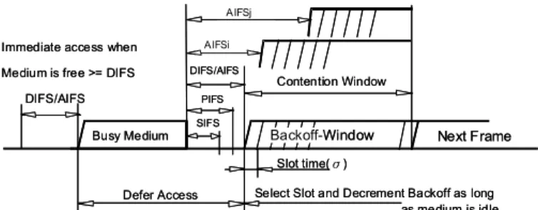
The access mechanism of 802.11e EDCF, as shown in Fig. 1, is similar to that of DCF. Four different priorities, called access categories (ACs), are supported in EDCF. Each AC has its associated values of CWmin, CWmax, and arbitration IFS (AIFS). The AIFS for the i-th AC, denoted by AIFSi, is defined by AIFSi=SIFS+Li × σ, for 1≦i≦4, (2)

26 where Li is an integer ranging from 1 to 255. Specifically, AIFSi is PIFS and DIFS for Li equal to 1 and 2, respectively. One should note that an AC with a smaller CWmin or AIFS implies a higher priority to access the channel. In EDCF, the backoff counter for priority i, denoted by ci, is modified as

ci = Rand (0,wi-1) + X, for 1≦i≦4, (3)

where wi is the CW for priority i; X is equal to 1 if Li=1, otherwise, it’s set to be 0. X is introduced to ensure

that operation of EDCF mode will not disturb the PCF mode.

Figure 1. Basic access mechanism under 802.11e EDCF MAC protocol.

III. T

HEORETICAL

A

NALYSIS

In this section, we investigate the weighted fairness of 802.11 under EDCF mode. We consider a system with NL low-class STAs and NH high-class STAs, each STA adopts a full queue traffic model [7]. For backward compatible to DCF, AIFSH=PIFS and AIFSL=DIFS are assigned for the two classes. An ideal channel condition without hidden terminals and with error-free transmission is assumed. We adopted the weighted fairness function given by [6]

, (4) H H L L ST ST φ φ =

where 　

φ

_H,

φ

_L,ST_H, and ST_L are the assigned weights and the successful transmission probabilities for high- and low-class STAs, respectively. We assumed that the average frame length for both classes is the same. Therefore, the traffic flows for each class may share the channel according to the pre-defined weights and the weighted fairness is then achieved if Eq. (4) can be guaranteed.

A. System Parameters and Observation Points

According to the backoff procedure, the decrement of backoff counter is stopped if the channel is sensed busy. Therefore, the time interval between two consecutive backoff counter decrements is not fixed. Due to the fact that AIFSH<AIFSL, we define a slot time as the (variable) time interval between two consecutive

AIFSj AIFSi DIFS/AIFS Contention Window Slot time(σ) Busy Medium Defer Access Next Frame

Select Slot and Decrement Backoff as long

SIFS PIFS

DIFS/AIFS Immediate access when Medium is free >= DIFS

as medium is idle Backoff-Window AIFSj AIFSi DIFS/AIFS Contention Window Slot time(σ) Busy Medium Defer Access Next Frame

Select Slot and Decrement Backoff as long

SIFS PIFS

DIFS/AIFS Immediate access when Medium is free >= DIFS

as medium is idle

27 backoff counter decrements for the high-class STAs. The observation points are then selected at the end of each time slot such that the backoff counter for either low- or high-class STAs can only be decreased at the observation points.

Let c n_L( ) and c n_H( ) be the stochastic processes representing the backoff counter of a given low- and high-class STA saw at the observation point n, respectively. The first property we found is that the c nH( ) is

always decreased but c nL( ) could be frozen for any observation point n. Since AIFSH=PIFS, the new

backoff counter for high-class STAs is initially chosen in range of (1,WH ) after a successful or a collided _i

transmission. However, the selection of initial backoff counter of a high-class STA must be done in a slot and should be decreased by 1 at the observation point. Thus, we have the second property that c n_H( )will fall into the range of (0,WH -1). _i

( ) L

c n and c n_H( ) are non-Markovian because the backoff counter depends also on its retransmission history. Therefore, we adopt the definition of “backoff stage,” which is defined as the number of retransmission attempts for a frame, to account for the retransmission history [8]. Let M_L (M_H) and WL ₀

(WH ) be the maximum backoff stage and the CWmin of the low-class (high-class) STAs, respectively. We ₀

can calculate the CW of the low-class (high-class) STAs at the i-th backoff by WL =2i×_i WL (₀ WH _i

= 2i_×

0

WH ), where i is called the backoff stage and i≦M_L (M_H).

B. Behavior of a Single Station with Different AIFS

Lets n_L( ) and s n_H( ) be the stochastic processes representing the backoff stage for a given low-class (high-class) STA at time n, respectively. We first consider the behavior of a single low-class STA with c n_L( )

and s n_L( ) at observation point n. Similar to the approximation adopted in [8], we assume that at each transmission attempt, each frame (of a low-class STA) collide with a constant and independent probability

L

P regardless of the number of retransmissions. P_L is referred to as conditional collision probability of a low-class STA, meaning that a collision seen by a frame (of a low-low-class STA) being transmitted on the channel. In other words, it is the probability that at least one of the other STAs (i.e. N_H high-class STAs and N_L-1 low-class STAs) counts down to zero while the low-class STA transmits. We further assume that a low-class STA with nonzero backoff counter may sense the channel as busy with a constant and independent probability q. q is referred to as channel busy probability sensed by a low-class STA. In other words, it’s the probability that at least one of other STAs (i.e. N_H high-class STAs and N_L-1 low-class STAs) transmits

28 while the low-class STA has nonzero backoff counter. Therefore, q is independent of the number of retransmissions.

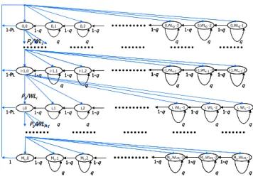
Once independence is assumed, and P_L and q are supposed to be constant values, it is possible to model the bi-dimensional process {s n_L( ),c n_L( )} with the discrete-time Markov chain as depicted in Fig. 2. Here, we assumed that the CW of a frame originates from a low-class (high-class) STA will be reset to WL (₀ WH ) ₀

if has been retransmitted for M_L (M_H ) times. In this Markov chain, the non-null one-step transition probabilities of a single low class station are

0 0 { , | , } , (1, 1) (0, ), (5) { , | , 1} 1 , (0, 2) (0, ), (6) {0, | ,0} (1 ) / , (0, 1), (0, 1), (7) { , | 1,0} i L i L L L P i k i k q k WL i M P i k i k q k WL i M P k i P WL k WL i M P i k i = ∈ − ∈ + = − ∈ − ∈ = − ∈ − ∈ − − = 0 0 / , (0, 1) (1, ), (8) {0, | ,0} 1/ , (0, 1). (9) L i i L L P WL k WL i M P k M WL k WL      _{∈ − ∈}   = ∈ −  where P i k i k{ , | , }_{1 1 0 0} ≡P s n{ ( + =1) i c n₁, ( + =1) k s n₁| ( )=i c n₀, ( )=k₀}. q q q q q ML,0 1-q ML,1 1-q ML,2 1-q ML,WLML-31-q ML,WLML-2 1-q ML,WLML-1 1-q 1 PL/WLi i,0

1-q i,1 1-q i,2 1-q 1-q i, WLi -3 1-q i, WLi -2 1-q i, WLi -1

1-PL

q q q q q

i-1,0

1-q i-1,1 1-q i-1,2 1-q 1-q i-1,WLi-1 -3 1-qi-1,WLi-1 -2 1-q i-1,WLi-1-1

1-PL PL/WLi+1 q q q q q 0,0 1-q 0,1 1-q 0,2 1-q 1-q 0,WL0 -3 1-q 0,WL0 -2 1-q 0,WL0-1 1-PL PL/WL1 q q q q q q q q q q ML,0 1-q ML,1 1-q ML,2 1-q ML,WLML-31-q ML,WLML-2 1-q ML,WLML-1 1-q 1 q q q q q ML,0 1-q ML,1 1-q ML,2 1-q ML,WLML-31-q ML,WLML-2 1-q ML,WLML-1 1-q ML,WLML-3 1-q ML,WLML-2 1-q ML,WLML-1 1-q 1 PL/WLi i,0

1-q i,1 1-q i,2 1-q 1-1-qq i, WLi -3i, WLi -3 1-1-qq i, WLi -2i, WLi -2 1-1-qq i, WLi -1i, WLi -1

1-PL

q q q q q

i-1,0

1-q i-1,1 1-q i-1,2 1-q 1-q i-1,WLi-1 -3 1-qi-1,WLi-1 -2 1-q i-1,WLi-1-1

1-PL

q q q q q

i-1,0

1-q i-1,1 1-q i-1,2 1-q 1-1-qq i-1,WLi-1 -3i-1,WLi-1 -3 1-1-qqi-1,WLi-1 -2i-1,WLi-1 -2 1-1-qq i-1,WLi-1-1i-1,WLi-1-1

1-PL PL/WLi+1 q q q q q 0,0 1-q 0,1 1-q 0,2 1-q 1-1-qq 0,WL0 -30,WL0 -3 1-1-qq 0,WL0 -20,WL0 -2 1-1-qq 0,WL0-10,WL0-1 1-PL PL/WL1 q q q q q

Figure 2. Markov chain model for the backoff counter with AIFSL=DIFS.

Letbi k_, =limn→∞Pr{ ( )s nL =i c n, ( )L =k i}, ∈(0,ML),k∈(0,WLi−1) be the steady-state probability of the low-class STA. We

can derive bi,k and b0,k by

,0 1,0 0,0, (1, ), (10) i i L i L L b =P b⋅ − =P b⋅ i∈ M 0,0 , ( ) , (1, ), (1, 1), (11) (1 ) i i L i k L i i WL k P b b i M k WL WL q − ⋅ ⋅ = ∈ ∈ − ⋅ − 0 0,0 0, 0 0 ( ) , (1, 1). (12) (1 ) k WL k b b k WL WL q − ⋅ = ∈ − ⋅ −

29 0,0 1 1 0 2(1 )(1 2 )(1 ) . (13) (1 )(1 (2 ) L ) (1 2 )(1 2 )(1 L ) L L M M L L L L q P P b WL P P + q P P + − − − = − − + − − −

Similarly, consider the stochastic process c n_H( ) and s n_H( ) for a high-class STA observed at n. We also assumed that at each transmission attempt, each frame (of a high-class STA) collide with a constant and independent probability P_H regardless of the number of retransmissions. P_H is referred to as conditional collision probability of a high-class STA, meaning that a collision seen by a frame (of a high-class STA) being transmitted on the channel. In other words, it’s the probability that at least one of the other STAs (i.e.

NH–1 high-class STAs and NL low-class STAs) counts down to zero while the high-class STA transmits.

PH is supposed to be a constant value because of the independence assumption. It is also possible to model

the bi-dimensional process {s n_H( ),c n_H( )} with the discrete-time Markov chain as depicted in Fig. 3. Similarly, the non-null one-step transition probabilities are

0 0 0 { , | , 1} 1, (0, 2) (0, ), (14) {0, | ,0} (1 ) / , (0, 1) (0, 1), (15) { , | 1,0} / , (0, 1) (1, ), (16) {0, | ,0} 1/ , (0, i H H H H i i H H P i k i k k WH i M P k i P WH k WH i M P i k i P WH k WH i M P k M WH k + = ∈ − ∈ = − ∈ − ∈ − − = ∈ − ∈ = ∈ WH₀ 1). (17)       ₋  i-1,WHi-1-3 1 i-1,WHi-1-2 1 i-1,WHi-1-1 1 i-1,0 1 i-1,1 1 i-1,2 1 i,WHi-3 1 i,WHi-2 1 i,WHi-1 1 i,0 1 i,1 1 i,2 1 1-PH 1-PH MH,WLMH-3 1 MH,WLMH-2 1 MH,WLMH-1 1 MH ,0 1 MH,1 1 MH,2 1 1 0,WH0-3 1 0,WH0-2 1 0,WH0-1 1 0,0 1 0,1 1 0,2 1 1-PH PH/WH0 PH/WHi PH/WHi+1 i-1,WHi-1-3 1 i-1,WHi-1-2 1 i-1,WHi-1-1 1 i-1,0 1 i-1,1 1 i-1,2 1 i,WHi-3 1 i,WHi-2 1 i,WHi-1 1 i,0 1 i,1 1 i,2 1 1-PH 1-PH 1-PH 1-PH MH,WLMH-3 1 MH,WLMH-2 1 MH,WLMH-1 1 MH ,0 1 MH,1 1 MH,2 1 1 MH,WLMH-3 1 MH,WLMH-2 1 MH,WLMH-1 1 MH ,0 1 MH,1 1 MH,2 1 MH,WLMH-3 1 MH,WLMH-2 1 MH,WLMH-1 1 MH ,0 1 MH,1 1 MH,2 1 11 0,WH0-3 1 0,WH0-2 1 0,WH0-1 1 0,0 1 0,1 1 0,2 1 0,WH0-3 1 0,WH0-2 1 0,WH0-1 1 0,0 1 0,1 1 0,2 1 1-PH 1-PH PH/WH0 PH/WHi PH/WHi+1

Figure 3. Markov chain model for the backoff counter with AIFSH=PIFS.

Here, we do not have P{i,k|i,k} as in Eq.(5) due to the first observed property that c n_H( ) is always decreased but c n_L( ) could be frozen for any observation point n. Also, the range of c n_H( ) (i.e. k) has to be modified to (0,WHi-1) according to the second observed property.

30 ,0 1,0 0,0, (1, ), (18) i i H i H H d =P d⋅ ₋ =P ⋅d i∈ M 0,0 , ( ) , (1, ), (0, 1), (19) i i H i k H i i WH k P d d i M k WH WH − ⋅ = ∈ ∈ − 0 0,0 0, 0 0 ( ) , (0, 1). (20) k WH k d d k WH WH − ⋅ = ∈ −

And, d0,0 can be found as

0,0 1 1 0 2(1 2 )(1 ) . (21) (1 )(1 (2 ) H ) (1 2 )(1 H ) H H M M H H H H P P d WH P P + P P + − − = − − + − −

C. Frame Transmission Probabilities with Different AIFS

Denote τ as the transmission probability that a high-class STA transmits in a randomly chosen time slot, _H

H

τ can be obtained by summarizing of the state probability di,0 found in (18) as

,0 0 1 1 0 2(1 2 ) . (22) (1 )(1 (2 ) ) /(1 ) (1 2 ) H H H M H i i H M M H H H H d P WH P P P P τ = + + = − = − − − + −

∑

Since AIFSH<AIFSL, the low-class STA may not affect the high-class STA. Therefore, τ is equal to the _H probability that more than one high-class STA that choose the same backoff counter. Similarly, we can derive the probability that more than one low-class STA that choose the same backoff counter value, denoted by

τ

'L, as ' 0 0 0 1 1 0 2 (2 1) 2(1 2 ) . (23) (1 )(1 (2 ) ) /(1 ) (1 2 ) L L L L M i L i L M i i L i L M M L L L L P P WL P WL P P P P τ = = + + ⋅ = ⋅ + − = − − − + −

∑

∑

The transmission probability that a low-class STA transmits in a randomly chosen time slot, denoted by

τ

L, is the sum of bi,0 found in (10) and is given by

,0 0 1 1 0 2(1 )(1 2 ) . (24) (1 )(1 (2 ) )/(1 ) (1 2 )(1 2 ) L L L M L i i L M M L L L L b q P WL P P P q P τ = + + = − − = − − − + − −

∑

Then we can derive the PH, PL, and q based on their definition. PH is the probability that a ready-to-transmit high-class STA collides with any of the NH-1 high-class STAs or NL low-class STAs. q is the probability that the channel is sensed busy by a low-class STA with nonzero backoff counter. The channel will be busy if any of the NH high-class STAs or NL-1 low-class STAs transmits at the same time. PL is the

31 probability that a ready-to-transmit low-class STA collides with any of the NH high-class STAs or NL–1 low-class STAs. In this case, the transmission probability for low-low-class STAs is

τ

'L because the counter of the ready-to-transmit low-class STA is zero. Then we can have,

1 1 ' 1 1 (1 ) (1 ) , 1 (1 ) (1 ) , (25) 1 (1 ) (1 ) . H L H L H L N N H H L N N L H L N N H L P P q τ τ τ τ τ τ − − −  = − − −  = − − −   _{= − − −} 

Finally, we can easily derive successful transmission probabilities of high-class and low-class STAs, respectively, as (1 ), (26) (1 ). H H H L L L ST P ST P τ τ = ⋅ −   _{= ⋅ −} 

Comparing with Eq. (4), we can use the numerical method to find the relationship between WH0 and WL0 from Eqs.(22), (23), (24), and (25) that can satisfied with Eqs. (4) and (26) by fixing the values of

φ

H,

φ

L, NH,

NL, MH, and ML.

IV.

NUMERICAL RESULTS

To validate the analysis, simulations were performed based on MATLAB. The values of PHY-related parameters were referred to IEEE 802.11b [9]. The symbol transmission rate was set to 11 Mbps. The frame format was the one defined by the 802.11e MAC specifications, and the PHY header and IFS intervals were those defined for 802.11b PHY. The PHY overhead time including preamble and header length is 196 µs, σ is 20 µs, SIFS is 10 µs, and the propagation delay is 1 µs. The length of the MAC header and ACK packet is 36 and 14 bytes, respectively. Unless otherwise specified, a constant frame payload size of 1028 bytes, which includes 1000 bytes application data payload, 20 bytes IP header, and 8 bytes UDP header, were used in the simulations. The full queue traffic model was assumed to apply to all stations. The maximum backoff stage

MH and ML were both set to be equal to 5 throughout this section. Unless otherwise specified, the numerical results were depicted in solid and dash lines and the simulation results were depicted with hollow and full symbols.

The accuracy of the analysis is verified by simulation results. In the following examples, we fix the sum of

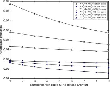
NH and NL to be 10 and set WL0 to be 32. The effect of high- and low-class STAs (i.e. NH and NL, respectively) for different values of WH0 was investigated. In Fig.4, the transmission probabilities of the two classes (i.e.

τ

H and

τ

L) were depicted for different NH and WH0. It was found that the larger NH would lead to smaller transmission probabilities for both classes because the high-class STAs have more chances to access the

32 channel. It was observed that, if WL0 was fixed, a small WH0 resulted in a high

τ

H but a low

τ

L. Fig. 5 showed the weighted fairness, STH/STL, for different cases. It was showed that STH/STL was highly depended on the selection of (WH0, WL0). The smaller WH0 would lead to the larger STH/STL when WL0 was fixed. Moreover, the growth of NH might lead to the decrease of STH/STL. Moreover, it was found that, the STH/STL could be greater than one even if WH0=WL0. The differentiation of throughput was achieved by setting different AIFSs.

Based on the results observed above, we might choose a suitable WL0 based the given NH, NL, MH, and ML. Then we may adopt any numerical method to find the WH0 based on the desired weighted goal

φ

H/

φ

L. In the simulations, WH0 was initially set to be equal to WL0. For a given WH0, STH/STL was calculated. The new value of WH0 was decreased if STH/STL <

φ

H/

φ

L and was increased otherwise. The iteration continued until |STH/STL-

φ

H/

φ

L| was minimized.

In the following, we show that the fairness is achieved using the proposed method. A total of 10 STAs are considered. The weighted goal

φ

H/

φ

L is 2 and the WL0 is fixed to be 32. WH0 is then chosen based on the weighted goal for different combination of (NH, NL). Fig. 6 showed that the weight goal was achieved for different combination of high- and low-class STAs. Due to the constraint that WH0 was an integer, therefore, it resulted in a little fluctuation of STH/STL.

V.

CONCLUDING REMARKS

In this paper, we proposed an analytical method to obtain parameters required to achieve weighted fairness for services operating under the enhanced distributed coordinator function (EDCF) mode. A system with full queue traffic model and supported two classes of services was considered. Specifically, the length of AIFS was set to be DIFS and PIFS for low- and high-class stations, respectively, to backward compatible with 802.11. In the queueing analysis, a discrete-time Markov-chain was adopted to model the behavior of backoff counters for the two classes and the steady-state probabilities were derived. We further explored the relationship between throughput, conditional collision probability, and conditional busy medium probability for the two classes. With the information, the size of the contention window was adjusted to achieve the weighted goal. The accuracy of the analytical solution is verified by simulation for different number of active stations. It can conclude that, for different combination of high- and low-class STAs, the weighted fairness is easily achieved by employing the proposed method.

33

REFERENCES

[1] G. Bianchi, L. Fratta, and M. Oliveri, “Performance Evaluation and Enhancement of the CSMA/CA MAC Protocol for 802.11 Wireless LANs,” IEEE PIMRC, Taipei, Taiwan, Oct. 1996, pp. 407-411.

[2] F.Cali, M.Conti, and E.Gregori, “Dynamic Tunig of the IEEE 802.11 Protocol to Achieve a Theoretical Throughput Limit,” IEEE/ACM Trans. on Networking, vol. 8, no. 6, Dec. 2000.

[3] H. Wu, S. Cheng, Y. Peng, K. Long, and J. Ma, “IEEE 802.11 Distributed Coordination Function (DCF) Analysis and Enhancement,” IEEE ICC, vol. 1,pp. 605-609, 2002.

[4] N. H. Vaidya, P. Bahl, and S. Gupta, “Distributed Fair Scheduling in Wireless LAN,” IEEE MOBICOM, Boston, MA, Aug. 2000, pp. 167-178.

[5] A. Banchs and X. Perez, ”Distributed Weighted Fair Queuing in 802.11 Wireless LAN,” IEEE ICC, vol. 5 , pp. 3121 -3127, 2002.

[6] D. Qiao and K.G. Shin, ”Achieving Efficient Channel Utilization and Weighted Fairness for Data Communications in IEEE 802.11 WLAN under the DCF ” Tenth IEEE International Workshop on Quality of Service, pp. 227 -236, 2002.

[7] 3GPP TSG-RAN-1, Nortel Networks, “Nortel Networks’ reference simulation methodology for the performance evaluation of OFDM/WCDMA in UTRAN”, Document R1-03-0518, Meeting #32, Paris, France, May 19-23, 2003.

[8] G. Bianchi, “Performance Analysis of the IEEE 802.11 Distributed Coordination Function,” IEEE Journal on Selected Area in Communications, vol.18, no.3, pp. 535-547, Mar. 2000.

[9] “IEEE Standard for Wireless LAN Medium Access Control (MAC) and Physical Layer (PHY) specifications: Higher-Speed Physical Layer Extension in the 2.4 GHz Band,” IEEE Std 802.11b-1999, Sep. 1999.

34 1 2 3 4 5 6 7 8 9 0.01 0.02 0.03 0.04 0.05 0.06 0.07 0.08 0.09

Number of high-class STAs (total STAs=10)

T ra ns m is si on pr obabi lit y WH 0=16,WL0=32,high-class WH 0=16,WL0=32, low-class WH 0=24,WL0=32,high-class WH 0=24,WL0=32, low-class WH 0=32,WL0=32,high-class WH 0=32,WL0=32, low-class

Figure 4. Transmission probability: analytical versus simulation results.

1 2 3 4 5 6 7 8 9 1 1.5 2 2.5 3 3.5 4 4.5 ST H /S TL

Number of high-class STAs (total STAs=10)

WH₀=16,WL₀=32 WH₀=24,WL₀=32 WH₀=32,WL₀=32

Figure 5. The STH/STL: analytical versus simulation results.

1 2 3 4 5 6 7 8 9 1.8 1.9 2 2.1 2.2

Number of high-class STAs (total STAs=10)

ST H /ST L ideal weighted numerical results

35

A Joint Power and Rate Assignment Algorithm

for Multirate Soft Handoff

in WCDMA Heterogeneous Cellular Systems

Ching-Yu Liao, Chung-Ju Chang, and Yi-Shen Chen

Department of Communication Engineering

National Chiao Tung University

Hsinchu 300, Taiwan ROC

E-mail: [email protected]

Tel. No.: 886-3-5731923 Fax No.: 886-3-5710116

Department of Communication Engineering,

National Chiao Tung University, Taiwan, ROC. Email: [email protected]

Tel: +886-3-5731923 Fax: +886-3-5710116

Abstract

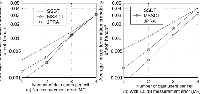
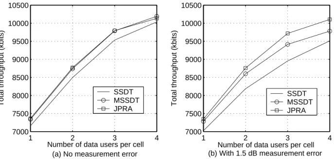
The paper proposes a joint power and rate assignment (JPRA) algorithm to deal with multirate soft handoff in WCDMA heterogeneous cellular systems. This JPRA algorithm, containing a constrained unequal power allocation (CUPA) scheme and an evolutionary computing rate assignment (ECRA) method, can determine an appropriate allocation of power and service rate for multirate soft handoffs, respectively. It can achieve power balancing between cells for soft handoffs better than the conventional site-selection diversity transmission (SSDT) scheme. Simulation results show that the JPRA algorithm can improve the forced termination probability of soft handoffs by 61.0 %, and the total throughput by 2.4 %. Besides, considering measurement error happened during the active set selection, the JPRA algorithm can further improve the forced termination probability of soft handoffs by 76.8 %, and the total throughput by 6.7 %.

Keywords

multirate soft handoff, heterogeneous cellular system, power allocation, rate assignment.

36

I. Introduction

Soft handoff is one of the most important features in WCDMA cellular mobile communication systems. When mobile users move from one cell to another cell, the soft handoff technique can provide seamless connections and better signal qualities for users in the cell boundary. However, in the forward link, systems often have to consume more power to serve soft handoff users than that to serve non-handoff users. Since the power resource are shared between non-non-handoff users and soft non-handoff users, the radio resource management would be a critical problem especially when soft handoff users are with multirate services. Generally, a multirate soft handoff costs much more power resource to satisfy the required quality of service.

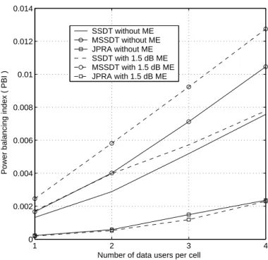
Furthermore, in heterogeneous WCDMA cellular systems, microcells, which are with stringent power budget, may easily exhaust their total transmission power because of serving soft handoff users in the forward link [1], [2], [3], and then there is no extra power resource for serving other users in the system. This situation would become worse for multirate WCDMA heterogeneous cellular systems. If power balancing can be achieved between macrocells and microcells through effectively managing radio resources for multirate soft handoffs, there are more power resource can be allocated for users in the congested microcells. Consequently, the system performance can be improved.

In this paper, we propose a joint power and rate assignment (JPRA) algorithm for multirate soft handoff users in WCDMA heterogeneous cellular systems. Many literature discussed the issue of joint power and rate assignment for all users in the cellular system in the sense of global optimization problem [4], [5]. However, they focused on the reverse link and did not concern about multirate soft handoffs. Reference [6] discussed radio resource management in multiple-chip-rate direct sequence CDMA systems supporting multiclass services, and it developed call admission control to arrange handoff in the same subsystem or execute inter-frequency handoff. Kim [7] dealt with rate-regulated power control in the reverse link without concerning handoff. Kim and Sung [8] proposed a handoff management scheme for multirate services using guard channels and reservation on demand queue control. But a hard handoff scheme was considered. Reference [9] and [10] proposed joint power and rate allocation algorithms in the downlink CDMA systems, however no handoff mechanism was concerned.

The proposed JPRA algorithm is composed of a two-phase process. In the first phase, a constrained unequal power allocation (CUPA) scheme is designed for soft handoffs. A conventional site selection diversity transmission (SSDT) scheme was proposed for soft handoff in [11]. It dynamically selects one base station with best link quality in the active set to serve the soft handoff. The SSDT sometimes cannot offer enough power required for multirate soft handoff users because of the maximum allocation

37 power constraint. Furthermore, since SSDT is a single site transmission scheme at one time, it easily consumes more power when suffering measurement error during active set selection. The advantage of power saving feature would disappear. The proposed CUPA is a multi-site diversity transmission scheme. It distributes the required allocation power for one soft handoff user unequally among all the active base stations, based on link quality between the active base station and the soft handoff user. The base station with better link quality will allocate more power than others with worse link qualities. In addition, the allocation power is constrained by the maximum allocation power of the base station. In the second phase of JPRA algorithm, an evolutionary computing rate assignment (ECRA) method is proposed to formulate an integer and discrete optimization problem under a predefined total power constraint for soft handoffs in each cell. It is well known that conventional optimization methods can hardly cope with problems with integer and discrete variables, whereas evolutionary computing methods are very efficient for these problems for reducing the searching complexity [12].

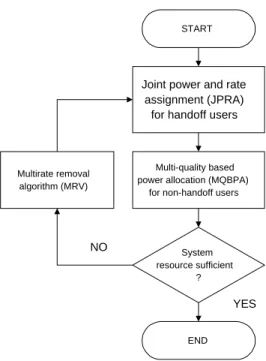
In the meantime, a multirate removal (MRV) algorithm is proposed to pick out a user who consumes system resource most and to reduce its service rate or even block it when the system resource is insufficient. Several removal algorithms had been proposed. Among these, the link-based and received signal-strength based removal algorithms were only suitable for single service [13], [14]. The prioritized removal algorithm, based on predefined service priority, did not consider service rate tuning for users in the reverse link of a multiservice cellular system [15]. On the other hand, a new multi-quality balancing power allocation (MQBPA) algorithm for non-handoff users with multiple service rates is also developed. Previous work for quality balancing power allocation technique were studied only for a single service rate and the same required signal quality [1], [3], [16]. Consequently, system operation for forward-link power and rate assignment containing JPRA for soft handoff is shown in Figure 1.

Simulation results show that proposed JPRA algorithm effectively achieves power balancing between macrocells and microcells in WCDMA heterogeneous cellular systems. Because of the power balancing characteristic, JPRA can improve not only the forced termination probability of soft handoffs by 61.0 % but also the total throughput by 2.4 %, as compared to the conventional SSDT scheme. Moreover, with the concern of 1.5 dB measurement error happened during the active set selection, it further improves the forced termination probability of soft handoffs by 76.8 %, and the total throughput by 6.7 %. The proposed JPRA algorithm can achieve better power balancing between cells and owns less sensitivity to the measurement error during the active set selection in multirate WCDMA heterogeneous cellular systems.

The remaining parts of this paper are organized as follows. In section II, the JPRA algorithm for multirate soft handoff is proposed. Simulation results are presented and discussed in section III.

38

YES Joint power and rate

assignment (JPRA) for handoff users

Multi-quality based power allocation (MQBPA)

for non-handoff users

END System resource sufficient ? NO START Multirate removal algorithm (MRV)

Fig. 1. The system operation of forward-link power and rate assignment

Finally, section VI concludes this paper. Moreover, the proof of CUPA convergence is provided in the Appendix A; the MQBPA and MRV algorithms are provided in the Appendix B and C, respectively.

II. The JPRA Algorithm

The JPRA algorithm is mainly composed of the constrained unequal power allocation (CUPA) scheme in the first phase and the evolutionary computing rate assignment (ECRA) method in the second phase. Before describing them, the received bit-energy-to-noise ratios of multirate soft handoff is defined.

In WCDMA cellular systems, the received bit-energy-to-noise ratio (Eb/No) of user j in base station i and with service rate r, denoted by γi,j(r), must be larger than or equal to the required signal quality, denoted by γ∗_{(r). For bandwidth W , the γ}

i,j(r) can be expressed as γi, j(r) = qi,j(r) · Li,j · G(r) P k Pk· Lk,j+ ηo ≥ γ∗(r) , (1)

where qi,j(r) is the allocation power from base station i to user j; Pk = N P j=1

qk,j is the total downlink transmission power for N users in cell k; Li,j is the link quality from cell i to user j; G(r) = W/r is the processing gain; and ηo is background noise. Assume that the link quality includes only the effect of both path loss and shadowing. For a soft handoff user h with service rate r, using the maximum

39 ratio combining (MRC) method to combine signals from all serving base stations in the active set Dh, its received Eb/No, γh(r), can be obtained by

γh(r) = X i∈Dh

γi,h(r). (2)

A. The CUPA Scheme

The constrained unequal power allocation (CUPA) scheme estimates the required allocation power for soft handoff user h, qh(r); then it distributes qh(r) to all serving base stations in Dh under the constraint of maximum allocation power to each user by base station i ∈ Dh, bqi. The qi,h(r) is pro-portional to the link quality between the serving base station i and the soft handoff user h [3]. If the allocation power of one link reaches to the constraint of maximum allocation power, the CUPA will compensate the required power through other links. The CUPA scheme is an iterative method to distribute qh(r) to all serving base stations so that the required signal quality can be satisfied. The design is to try to accomplish power balancing between cells in the heterogenous cellular system with different cell sizes. Besides, it is noteworthy that because of the maximum allocation power constraint of each forward link, there exists a forced termination situation for the soft handoff because the soft handoff user cannot obtain required signal quality even though all active links are allocated with max-imum power. If the soft handoff is forced to terminate, the qi,h(r) of each link i in the active set Dh are reset to zero. The CUPA scheme is stated in more details in the following.

[The CUPA Scheme]

Step 0: [Exam soft handoff feasibility]

• Allocate maximum power bq_i for each active links i .

• Calculate received signal quality γh(r) based on (1) and (2). • IF γ_h(r) > γ∗(r), THEN Goto Step 1.

ELSEIF γh(r) = γ∗(r), THEN Set qi,h(r) = bqi, i ∈ Dh, DONE.

ELSE the soft handoff user h is forced to terminate (qi,h(r) = 0, i ∈ Dh), DONE. Step 1: [Initialize]

• Initialize the required transmission power q_hn(r), n = 0, for soft handoff user h to be the summation of the maximum allocation power, bqi, of each serving base station i by

q0h(r) = X i∈Dh

b

qi. (3)