A Bayesian Approach to Video Object Segmentation via Merging 3-D Watershed
Volumes
Yu-Pao Tsai, Chih-Chuan Lai, Yi-Ping Hung, and Zen-Chung Shih
Abstract—In this letter, we propose a Bayesian approach to
video object segmentation. Our method consists of two stages. In the first stage, we partition the video data into a set of three-dimen-sional (3-D) watershed volumes, where each watershed volume is a series of corresponding two-dimensional (2-D) image regions. These 2-D image regions are obtained by applying to each image frame the marker-controlled watershed segmentation, where the markers are extracted by first generating a set of initial markers via temporal tracking and then refining the markers with two shrinking schemes: the iterative adaptive erosion and the veri-fication against a presimplified watershed segmentation. Next, in the second stage, we use a Markov random field to model the spatio-temporal relationship among the 3-D watershed volumes that are obtained from the first stage. Then, the desired video objects can be extracted by merging watershed volumes having similar motion characteristics within a Bayesian framework. A major advantage of this method is that it can take into account the global motion information contained in each watershed volume. Our experiments have shown that the proposed method has potential for extracting moving objects from a video sequence.
Index Terms—Markov random field, three-dimensional (3-D)
watershed volume, video object segmentation, watershed segmen-tation.
I. INTRODUCTION
V
IDEO object segmentation plays an important role in many advanced video applications (such as in MPEG-4 or in virtual reality), but still remains a challenging research topic. A popular approach to video object segmentation is to com-bine a technique for single image segmentation with a temporal tracking procedure [20]. Unfortunately, single image segmenta-tion is itself a very difficult problem (which may not be easier than video object segmentation). Other techniques in [12], [15] consider video sequences to be three-dimensional (3-D) signals and extend two-dimensional (2-D) methods to them, although the time axis does not play the same role as the spatial axis. The drawback of this technique is that a moving object in one frame must overlap with its corresponding object in the next frame. If the motion distance of the object is large, the object may become disconnected from one frame to the next. Most of the unsupervised segmentation algorithms only utilize low-level Manuscript received October 8, 2002; revised April 21, 2004. This paper was recommended by Associate Editor M. Strintzis.Y.-P. Tsai is with the Institute of Information Science, Academia Sinica, Taipei 115, Taiwan 30050, R.O.C., and is also with the Department of Com-puter and Information Science, National Chiao Tung University, Hsinchu 300, Taiwan 30050, R.O.C.
C.-C. Lai and Y.-P. Hung are with the Institute of Information Science, Academia Sinica, Taipei, Taiwan, R.O.C., and also with the Department of Computer Science and Information Engineering, National Taiwan University, Taipei 106, Taiwan 30050, R.O.C. (e-mail: [email protected]).
Z.-C. Shih is with the Department of Computer and Information Science, National Chiao-Tung University, Hsinchu, Taiwan 30050, R.O.C.
Digital Object Identifier 10.1109/TCSVT.2004.839973
features such as color, texture, motion, frame difference and histogram [9], [20]. However, without high-order information, semantic video object extraction is hard to achieve. Therefore, many researches have allowed a certain degree of human inter-action. For example, the methods introduced in [2], [4] require some human interaction for the initial segmentation of the first image in the video. In fact, almost all the automatic algorithms developed for extracting video objects have some limitations. For example, the automatic method proposed in [20] can only extract homogeneous regions, instead of complete objects.
Realizing that there exists no generic automatic algorithm ap-plicable to all kinds of video sequences, we focus on the problem of extracting video objects having similar motion characteristic. The method proposed in this letter consists of two stages: 1) generation of 3-D watershed volumes and 2) Bayesian merging of 3-D watershed volumes. Details of the two stages will bde-scribed in Sections II and III. Experimental results will be shown in Section IV, and the conclusion will be given in Section V.
II. GENERATION OF3-D WATERSHEDVOLUMES Watershed algorithm has been become popular technique for image segmentation [5], [13], [18]. In this letter, we apply wa-tershed technique to video object segmentation by constructing 3-D watershed volumes. Given a video clip
we can regard the data as one volume image. Our method first partitions the volume image into a set of 3-D watershed
vol-umes, where each 3-D watershed volume is a series of
cor-responding 2-D image regions. Fig. 1 shows the flowchart of our method for generating 3-D watershed volumes. These 2-D image regions are obtained by applying to each image frame the
marker-controlled watershed segmentation described in Step 2
of Section II-B. The procedure for generating 3-D watershed volumes can be divided into two phases: initial segmentation and temporal tracking. Details of these two phases are described below.
A. Initial Segmentation
In the initial phase, the first frame of the video clip is partitioned into a set of 2-D regions by applying the watershed
segmentation algorithm to the gradient image of . However, the basic watershed transformation tends to produce over-seg-mentation due to noise or local irregularities in the gradient image. Since overly segmented regions may not be reliable enough for the next phase of temporal tracking, we adopt a preprocessing method called “topographic simplification” to alleviate the over-segmentation problem. In our current implementation, the topographic surface of the gradient image is simplified by removing the local minima [19]. First, we apply a dilation operation with a structuring element of 2 1051-8215/$20.00 © 2005 IEEE
Fig. 1. Flowchart of generating 3-D watershed volumes.
2 pixels, i.e., let . Next, we apply to
a “reconstruction by erosion” [17] from , i.e.,
let . Notice that using a larger
can eliminate more local minima. Finally, we can obtain a reasonable segmentation of by applying the basic watershed transformation to the simplified gradient image .
In this letter, the above procedure of “topographic
simplifi-cation followed by watershed transformation” will be referred
to as the presimplified watershed segmentation, and will be ap-plied again to each subsequent frame for the purpose of refining the extracted markers, as described in Step 1.3.
B. Temporal Tracking
In the second phase, our algorithm repeats the following two steps for each subsequent frame in the video clip: 1) marker ex-traction and 2) marker-controlled watershed segmentation. The task of marker extraction is to extract reliable seed regions based on the segmented regions obtained from the previous frame. Given these reliable markers, the marker-controlled watershed segmentation can not only accurately extract the boundaries of the watershed regions, but also can detect newly emerging re-gions.
Step1—Marker Extraction: Marker extraction is crucial to
the success of the temporal tracking phase and deserves some special attention here. Our method for extracting markers con-sists of the following three substeps:
Step 1.1—Region label propagation by motion-based back-ward projection: First, initial markers are obtained by using
backward pixel projection based on backward motion vectors. That is, for each pixel in the current frame, we assign to the region label of the corresponding pixel in the previous frame to it. The correspondence is determined by using the backward motion vector . Here, we choose to use backward motion to avoid generating empty and conflicting areas in the current frame. The dense field of backward motion vectors is estimated by using a template-matching algorithm that adopts adaptive windows, similar to the one used in [6]. To save the computation time, we first estimate a sparse field of motion vectors at every 4 4 pixel spacing. Then, the dense pixel-wise motion vectors are computed using bilinear interpolation. The approximation error can be dealt with the following process.
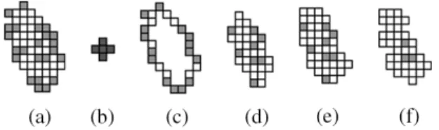
Fig. 2. Example of Step 1.2 for marker extraction. (a) Initial marker with unreliable pixels colored in grey. (b) Cross-shaped structuring element of 5 pixels. (c) Border pixels removed with the normal erosion. (d) Interior pixels obtained with the normal erosion. (e) Eroded marker after the first iteration of adaptive erosion. (f) After the second iteration (stable and stopped).
Step 1.2—Removing unreliable pixels from initial markers by iterative adaptive erosion: Since motion vectors are
usu-ally not very accurate, we must remove unreliable region assignments due to erroneous pixel correspondences. In order to reduce the possibility of generating false boundaries in the next substep, the extracted markers should be as large as possible, and completely contained in their true corresponding regions—which are unfortunately unknown to the computer.
Consider an initial marker . A pixel is regarded
as an unreliable pixel if it has an unreliable region propagation,
that is, if is greater than , where denotes the
local mean of textural error centered round pixel (that is, the error of texture, including intensity and color, between the cor-responding pixels)
(1)
where and its eight neighbors having the
same region label as p , is the number of elements in the set , and denotes the global mean of textural error for the whole area of marker
(2) where is the number of the pixels in marker . The reason for constraining to 2 and 16 is to prevent using an unreason-able large or unreasonunreason-able small threshold. The two numbers, 2 and 16, are determined according to our experiments.
In this substep, we apply an iterative adaptive erosion to trim off “unreliable border pixels” of the initial markers, as illustrated in Fig. 2. The adaptive erosion (erode if “unreliable”) is per-formed iteratively with a cross-shaped structuring element of 5 pixels, shown in Fig. 2(b), until the result becomes stable. No-tice that the adaptively eroded marker shown in Fig. 2(e) is a union of the normally eroded marker [shown in Fig. 2(d)] and the reliable pixels, colored in white, are contained in the border portions [shown in Fig. 2(c)].
Note that using a lower can eliminate more marker pixels. In the case of foreground and background objects, which are not distinctive, should be set conservatively. We found that works well for most MPEG-4 test sequences in hand. The resulting markers with different values of using frame 116 of the “foreman” sequence are shown in Fig. 3. Pixels in black represent any undefined areas.
Fig. 3. Markers extracted from frame 116 of sequence “foreman” with different the value ofk after Step 1.2 for marker extraction. (a) k = 0:8. (b) k = 1:2.
Fig. 4. Example of Step 1.3 for marker extraction. (a) Two different markers are overlaid by the watershed lines obtained from presimplified watershed segmentation. (b) The shrunk marker after removing the doubtful portions.
Fig. 5. Markers extracted from frame 116 of sequence “foreman” with different the value ofk after Step 1.3 for marker extraction. (a) k = 0:8. (b) k = 1:2.
Step 1.3—Removing unreliable pixels by checking with a presimplified watershed segmentation: Here, we first
gener-ated a reasonably fine segmentation of the current frame by applying the presimplified watershed segmentation described in Section II-A, with a small value of parameter . For each gen-erated watershed region, check if it contains only one marker and the sole marker occupies more than half of the watershed region. If so, the sole major marker will be retained for driving the marker-controlled watershed segmentation in the next step. Otherwise, the marker pixel in this watershed region will be considered “unreliable,” and will be removed from the markers, as illustrated in Fig. 4. Fig. 5 shows the final markers obtained by applying this substep to the markers shown on Fig. 3. We can see that after this step, small and ambiguous pieces of the marker are removed.
Step 2—Marker-Controlled Watershed Segmentation: Based
on the reliable markers obtained from the last step, we can then extract more precise region boundaries by using the
marker-controlled watershed segmentation [8], [20]. One problem
ac-companying marker-controlled segmentation is that no newly exposed regions can be extracted without creating new markers. To solve this problem, we modify the marker-controlled water-shed algorithm slightly. For the flooding process of the marker-controlled watershed algorithm used in [20], when the water
Fig. 6. New region is labeled if the dynamics of a catchment basin exceeds a certain threshold.
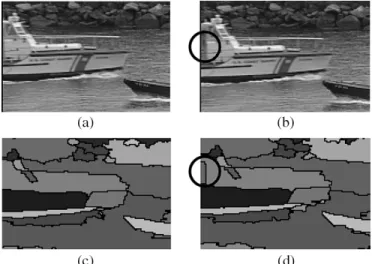
Fig. 7. Demonstration of detecting new region by using dynamic thresholding. (a) Frame 26. (b) Frame 27. (c) Segmented result of frame 26. (d) Segmented result of frame 27.
coming from two different basins is about to meet, the two basins are merged if “both have the same label” or “at least one of them is unlabeled.” Our modification for creating new markers is if the dynamics of an unlabeled basin larger than a certain threshold [7], [10], the basin will be given a new label (Fig. 6). Fig. 7 shows the result of detecting new regions using frame 26 and 27 of the “coastguard” sequence. The big boat is entering the image from the left, and the background water can be detected as a new region.
III. BAYESIANMERGING OFWATERSHEDVOLUMES Once the 3-D watershed volumes are generated, as described in Section II, we need to merge them into a set of desired video objects. Here, we propose a Bayesian approach to merging wa-tershed volumes having similar motion characteristics, hoping that more global motion information can be utilized within a formal framework. Here, we use a Markov random field (MRF) to model the spatial and temporal relationships among different watershed volumes. A closely related work is the one done by Gelgon and Bouthemy, which uses region-level MRFs to track a spatial image partition [3]. Another work proposed by Patras
et al. [12] labels watershed segments by MAP. The labeling
cri-terion is the maximization of the conditional a posteriori prob-ability of the labeling field given the motion hypothesis, the es-timate of the label field of the previous frame, and image in-tensities. However, our method is different from theirs, not only in how the MRF is applied (we employ the MRF after tracking while they do it before tracking), but also in how the class-con-ditional probability is modeled.
tion. We first decompose each watershed volume into a set
of regions , where
de-notes a region which can be obtained by intersecting frame
with the watershed volume , and are the indices
of the beginning frame and the ending frame of the watershed volume , respectively. Note that the indices of the beginning and ending frames of the watershed volumes can vary for the watershed volume due to the appearance or disappearance of objects in the scene.
In practical situations, image motion of a rigid object can be approximately modeled by a small number of motion parame-ters. If two regions roughly correspond to the same 3-D rigid object, the motion parameter should be about the same. From the above observation, we compute a motion parameter vector for each region by applying the least-median squares (LMedS) robust estimator [13] to the backward dense motion field obtained from Step 1.1 of Section II-B. The motion pa-rameters can be estimated by
(3) where is a parameterized motion field, is defined as the two-norm operator, and is the motion vector of pixel in frame . After the parameters for all the regions in the wa-tershed volume are determined, we can construct a motion
feature vector: . Notice that
the dimensionality of is , where is
the dimension of . In our current implementation, the motion characteristics of are described by a constant motion field,
that is, , where and and
are the coordinates of the mean motion vector.
B. Proposed Method
In this work, we assume that the number of video objects to be extracted (including the background objects) is known. Given
a set of 3-D watershed volumes , where
is the number of 3-D watershed volumes, a volume adjacency graph (VAG) can be constructed to express the neighborhood relationship among 3-D watershed volumes. Each node in the graph corresponds to a watershed volume, and between two vol-umes exists an arc if the volvol-umes are spatially connected. Next,
we define a label field on the
VAG. Given , we estimate the labeling field
by maximizing the a posteriori probability (MAP). Using the Bayes rule, the a posteriori probability density function can be expressed as
(4) The first term on the right-hand side of (4) is the conditional probability distribution . It is modeled as a Gaussian
where is the mean of the parameter vectors of all water-shed volumes in frame whose corresponding labels are , is a function of the size of the video object.
The second term on the right-hand side of (4) is the prior probability distribution , which is a regularization term. To take into account the “degree” of adjacency between two watershed volumes, we directly extend a measure of adjacency degree between two regions proposed in [3] to that between two watershed volumes
(6)
where is the area of the common border between
and , and and are the gravity centers of and ,
respectively. We model the prior as a Gibbs distribution. Before defining a Gibbs distribution, we need to define the cliques. Here, only two-site cliques are considered and straightfor-wardly obtained from the arc of the VAG. Let be the set of all binary cliques. The Gibbs distribution is given by
(7) where is a normalizing constant and , the regulariza-tion potential, is defined as
(8)
where is a Kronecker delta function. The regularization term tends to favor identical labels for two neighboring volume sites.
The maximum a posteriori probability (MAP) estimate of is obtained by minimizing the following energy function
(9) Energy minimization is performed using an ICM algorithm proposed by Besag [1], sometimes also called the greedy algo-rithm. At each iteration, each volume sites is visited. The label of each site is either changed to the label that yields maximal decrease of the energy function, or left unchanged if no energy reduction is possible. The process stops when no more changes can be made. The detail can be found in [16].
IV. EXPERIMENTALRESULTS
In this section, we use the “foreman”, and “coastguard” se-quences, shown in Figs. 8 and 9, respectively, to demonstrate the performance of our algorithm. The experiments are run on
Fig. 8. “Foreman” sequence: frame 1, 20, 40, 60, 80, 100. (a) Original images. (b) After temporal tracking. (c) After Bayesian merging.
AMD Athlon 1.2 GHz PC with 384 MB RAM. The sizes of the “foreman” sequence and the “coastguard” sequence are 352 288 and 352 240. As to the total execution time, the pro-cessing of the “foreman” sequence with 100 frames requires 483 s and the “coastguard” sequence with 50 frames requires 131 s. In our current implementation, the gradient images are
com-puted on a weighted YUV color space, i.e., .
The weighting factors, , , and , are set to one, two, and two, respectively, to emphasize the color components.
In the “foreman” sequence, the human body has a moderate motion and the camera is moving as well. It can be seen from Fig. 8(b), where cross-sections of watershed volumes are shown, that the results obtained by marker-controlled temporal tracking look pretty good. By setting (i.e., the number of video objects to be extracted is 2), the watershed volumes depicted in Fig. 8(b) can be correctly merged into two video objects: the foreman and the background, as shown in Fig. 8(c). In this se-quence, we have found that the similarity between the motions of the head and the shoulder could be more easily detected when
Fig. 9. “Coastguard” sequence: frame 1, 10, 20, 30, 40, 50. (a) Original Images. (b) After temporal tracking. (c) After Bayesian merging.
considering a longer sequence. Therefore, our method can ob-tain better segmentation results than those obob-tained by Moschni
et al. [9].
In the “coastguard” sequence, the horizontal camera drift is present while two boats are moving with different velocities and directions. Notice that the bigger boat is entering the image from the left, and its new emerging regions can be successfully ex-tracted, as shown in Fig. 9(b). If we set , the proposed Bayesian method can partition the video clip into four different objects: the bigger boat, the smaller boat, the water and the shore, as shown in Fig. 9(c). Compared with the results using the method proposed by Patras et al. [12], the segmented bound-aries we extracted are much closer to the objects.
V. CONCLUSION
In this letter, we have proposed a new method for video ob-ject segmentation. This method first partitions the video data into a set of 3-D watershed volumes, and then extracts video objects by merging motion-coherent watershed volumes within a Bayesian framework. One major contribution of this work is that it models the prior information with a MRF over a volume adjacency graph (VAG), where each node of the VAG is a 3-D watershed volume and, hence, is able to take into account the global motion information contained in each watershed volume.
segmentation. Experimental results have shown that the pro-posed method has potential for extracting moving objects from a video sequence.
REFERENCES
[1] J. Besag, “On the statistical analysis of dirty pictures,” J. R. Stat. Soc. B, vol. 48, no. 3, pp. 259–302, 1986.
[2] D. Gatica-Perez, G. Gu, and M.-T. Sun, “Semantic video object extrac-tion using four-band watershed and partiextrac-tion lattice operators,” IEEE
Trans. Circuits Syst. Video Technol., vol. 11, no. 5, pp. 603–618, May
2001.
[3] M. Gelgon and P. Bouthemy, “A region-level motion-based graph rep-resentation and labeling for tracking a spatial image partition,” Pattern
Recognit., vol. 30, no. 4, pp. 725–740, 2000.
[4] C. Gu and M. Lee, “Semiautomatic segmentation and tracking of se-mantic video objects,” IEEE Trans. Circuits Syst. Video Technol., vol. 8, no. 5, pp. 572–584, May 1998.
[5] K. Haris, S. N. Efstratiadis, N. Maglaveras, and A. K. Katsaggelos, “Hy-brid image segmentation using watersheds and fast region merging,”
IEEE Trans. Image Process., vol. 7, no. 12, pp. 1684–1699, Dec. 1998.
[6] T. Kanade and M. Okutomi, “A stereo matching algorithm with an adap-tive window: theory and experiment,” IEEE Trans. Pattern Anal. Mach.
Intell., vol. 16, no. 9, pp. 920–932, Sep. 1994.
[7] C. Lemarechal and C. Fjortoft, “Comments on “Geodesic saliency of watershed contours and hierarchical segmentation’,” IEEE Trans.
Pat-tern Anal. Mach. Intell., vol. 20, no. 7, pp. 762–763, Jul. 1998.
[11] M. Pardas and P. Salembier, “3-D morphological segmentation and motion estimation for image sequences,” Signal Process., vol. 38, pp. 31–43, 1994.
[12] I. Patras, E. A. Hendriks, and R. L. Lagendijk, “Video segmentation by MAP labeling of watershed segments,” IEEE Trans. Pattern Anal. Mach.
Intell., vol. 23, no. 3, pp. 326–332, Mar. 2001.
[13] J. B. T. M. Roerdink and A. Meijster, “The watershed transform: defini-tions, algorithms and parallelization strategies,” Fund. Inform., vol. 41, pp. 187–228, 2000.
[14] P. J. Rousseeuw, “Least median of squares regression,” J. Amer. Statist.
Assoc., vol. 79, pp. 871–880, 1984.
[15] P. Salembier and M. Pardas, “Hierarchical morphological segmentation for image sequence coding,” IEEE Trans. Image Process., vol. 3, no. 5, pp. 639–651, Sep. 1994.
[16] Y.-P. Tsai, C.-C. Lai, Y.-P. Hung, and Z.-C. Shih, “A Bayesian Approach to Video Object Segmentation via Merging 3-D Watershed Volumes,” Academia Sinica, Taiwan, R.O.C., Tech. Rep. TR-IIS-04-005, 2004. [17] L. Vincent, “Morphological grayscale reconstruction in image analysis:
application and efficient algorithms,” IEEE Trans. Image Process., vol. 2, no. 2, pp. 176–201, Feb. 1993.
[18] L. Vincent and P. Soille, “Watersheds in digital spaces: an efficient al-gorithm based on immersion simulations,” IEEE. Trans. Pattern Anal.
Mach. Intell., vol. 13, no. 6, pp. 583–598, Jun. 1991.
[19] D. Wang, “A multiscale gradient algorithm for image segmentation using watersheds,” Pattern Recognit., vol. 30, no. 12, pp. 2043–2052, 1997.
[20] , “Unsupervised video segmentation based on watersheds and tem-poral tracking,” IEEE Trans. Circuits Syst. Video Technol., vol. 8, no. 5, pp. 539–546, May 1998.