D Minimizing Total Earliness and Tardiness for Common Due Date Single-Machine Scheduling with an Unavailability Interval

Research Article

Minimizing Total Earliness and Tardiness for Common Due

Date Single-Machine Scheduling with an Unavailability Interval

Chinyao Low,

Rong-Kwei Li,

and Guan-He Wu

1_{Department of Industrial Engineering and Management, National Yunlin University of Science and Technology,}

123 University Road, Douliou, Yunlin 64002, Taiwan

2_{Department of Industrial Engineering and Management, National Chiao Tung University, 1001 University Road,}

Hsinchu 30010, Taiwan

Correspondence should be addressed to Chinyao Low; lowcy@yuntech.edu.tw Received 23 March 2016; Accepted 6 June 2016

Academic Editor: Miguel A. Salido

Copyright © 2016 Chinyao Low et al. This is an open access article distributed under the Creative Commons Attribution License, which permits unrestricted use, distribution, and reproduction in any medium, provided the original work is properly cited.

This paper addresses the problem of scheduling𝑛 independent jobs on a single machine with a fixed unavailability interval, where

the aim is to minimize the total earliness and tardiness (TET) about a common due date. Two exact methods are proposed for solving the problem: mixed integer linear programming formulations and a dynamic programming based method. These methods are coded and tested intensively on a large data set and the results are analytically compared. Computational experiments show that the dynamic programming method is efficient in obtaining the optimal solutions and no problems due to memory requirement.

1. Introduction

This paper considers the minimization of total earliness and tardiness (TET) for common due date single-machine scheduling with an unavailability interval. The TET perfor-mance measure is consistent with the just-in-time (JIT) man-ufacturing philosophy in which an ideal schedule consists of all jobs finish exactly on the due date.

These days, the emphasis on the JIT approach has led to a growing interest in earliness-tardiness scheduling models. In a JIT scheduling environment, job earliness may cause bounded capital and inventory holding costs, whereas job tardiness may disrupt a customer’s operations. Therefore, both earliness and tardiness should be taken into account in order to determine the optimal machine scheduling policy.

The common due date scenarios are relevant in many realistic situations; for example, several items constitute a customer order, or they are delivered to an assembly line where the components are all required to be ready at the same time. Numerous studies have been published on the earliness-tardiness scheduling problems with common due date, such as those discussed in the surveys of Baker and Scudder [1], Biskup and Feldmann [2], Gordon et al. [3], and Lauff and

Werner [4]. In what follows, some references related to the common due date TET minimization are recalled.

Kanet [5] proposed a polynomially bounded matching algorithm for the single-machine problem that the due date was assumed to be greater than the total processing time of the jobs. Bagchi et al. [6] extended Kanet’s result and provided an implicit enumeration procedure to find all the optimal schedules. Sundararaghavan and Ahmed [7] developed a polynomial-time algorithm to determine the optimal job-machine assignment for identical parallel job-machines. Emmons [8] investigated the uniform parallel-machine scheduling problem when the makespan and machine occupancy were considered as the secondary objective. Baker and Scudder [1] specified the minimum value of a common due date that gives rise to the unrestricted version of the TET problem. Dynamic programming algorithms and branch-and-bound methods for single-machine scheduling with a restricted due date were presented in [6, 9–13]. Sarper [14] modelled the two-machine flow shop scheduling problem as a mixed integer linear programming formulation and suggested three constructive heuristics. Sakuraba et al. [15] introduced a job timing algorithm for generating the optimal schedule when the sequence of jobs processed in the two-machine flow shop

Volume 2016, Article ID 6124734, 12 pages http://dx.doi.org/10.1155/2016/6124734

was given. Sung and Min [16] addressed the problem of scheduling two-machine flow shop with at least one batch processor incorporated. Some optimality properties were characterized for three different system configurations to derive their corresponding solution methods. Yeung et al. [17] proposed a branch-and-bound method and a heuristic to solve the two-machine flow shop scheduling problem with TET criterion in relation to a given common due window. Lauff and Werner [18] investigated the computational com-plexity of multistage scheduling problems with intermediate storage costs.

It can be observed that the majority of previous studies assumed that the machines are available at all times. However, in a real production system, machines may not be always available because of unforeseen breakdowns, tool changes, or preventive maintenance requirements for improving the production efficiency. It is also possible that machines have been committed to deal with the promised orders and hence become unavailable for processing in certain periods of the current planning horizon. Under such circumstances, the optimal production strategies can be quite different from those attained by classical models.

Due to the practical experience in production systems, there has been a great deal of efforts concentrated on scheduling problems with limited machine availability (see Lee et al. [19]; Schmidt [20]; Ma et al. [21]). More recently, Low et al. [22] presented heuristic approaches to minimize the makespan on a single machine that was periodically unavail-able. Mosheiov and Sidney [23] developed polynomial-time algorithms for scheduling a deteriorating maintenance activ-ity on a single machine with different objective functions. Zhao and Tang [24] analyzed the single-machine scheduling problem with simultaneous considerations of maintenance activities and job-dependent aging effect while minimizing the makespan.

´

Angel-Bello et al. [25] proposed a mixed integer pro-gramming formulation and an efficient heuristic approach for the single-machine makespan problem with availability constraints and sequence-dependent setup costs. Huo and Zhao [26] presented polynomial-time algorithms to optimize both makespan and total completion time under a two-parallel-machine environment with availability constraints. Yang et al. [27] provided a dynamic programming algorithm and a branch-and-bound method for minimizing the total completion time on a single machine in which job processing and maintenance activity had to be scheduled simultaneously. Lee and Kim [28] studied the single-machine scheduling problem with periodic maintenance and adopted a two-phase heuristic to minimize the number of tardy jobs. Yin et al. [29] examined the problem of scheduling jobs and common due date assignment on a single machine with a rate-modifying activity. They proposed some optimality conditions and developed polynomial-time algorithms for special cases.

Dong [30] presented a column generation based branch-and-bound method to schedule identical parallel machines in which the job sequence and the timing of shutdown operation were jointly optimized. Hsu et al. [31] considered the scheduling problem of minimizing the total completion

time and the total machine load on the unrelated paral-lel machines with three basic types of aging effect mod-els and deteriorating maintenance activities. They showed that all the addressed models are polynomial-time solv-able. Shen et al. [32] proposed polynomial-time algorithms to schedule identical parallel machines with nonsimulta-neous machine available time. Vahedi-Nouri et al. [33] developed a new binary integer programming formula-tion and a branch-and-bound method for minimizing the total completion time in single-machine scheduling with learning effect and multiple availability constraints. Xu and Yang [34] considered the two-parallel-machine scheduling problem with a periodic availability constraint. They pre-sented a mathematical programming model to minimize the makespan.

Hashemian et al. [35] addressed the makespan minimiza-tion for parallel-machine scheduling with multiple planned unavailability intervals. A mixed integer linear programming model and an implicit enumeration algorithm were designed to tackle the problem. Kaplano˘glu [36] adopted a multi-agent based approach for scheduling single machine with sequence-dependent setup times and machine maintenance, where both of the regular and irregular maintenance activities were considered. Rustogi and Strusevich [37] studied the single-machine scheduling problem incorporating positional and time-dependent effects, in which the machine was sub-ject to rate-modifying activities that split the jobs into groups. The aims were to minimize the makespan and the total completion time. Yin et al. [38] explored the single-machine batch scheduling problem with an unavailability interval. A dynamic programming algorithm was proposed for minimiz-ing the sum of total flow time and batch delivery cost. Yin et al. [39] investigated the problem of scheduling jobs with assignable due dates on a single machine, in which the job processing times were subject to positional deterioration and the execution of preventive maintenance. They analyzed the structural properties of the problems under consideration and presented polynomial-time algorithms for deriving the optimal solution. Rustogi and Strusevich [40] considered the single-machine scheduling problem with linear time-dependent deterioration effects and maintenance activities. A range of polynomial-time algorithms were designed to minimize the makespan.

Most of the aforementioned scheduling models focused on regular performance measures such as makespan, total completion time, and number of tardy jobs. With current emphasis on the JIT production strategy, these classical measures may no longer be applicable. So far, only Low et al. [41] addressed the problem of minimizing common due date TET in the presence of availability constraints. They developed an ant colony optimization algorithm for the single-machine model in which one maintenance task had to be performed and analyzed some special cases that are polynomial-time solvable. Nevertheless, such heuristic approaches offer no guarantees to the optimality of the obtained solutions and do not define how close the obtained solutions are to the optimal ones. Furthermore, it should be noted that the matching algorithm suggested by Low et al. [41] only can be used to deal with the cases when the due

date falls within the unavailability interval and certain con-ditions are satisfied. In practical scheduling environments, the production schedulers always expect to come up with an optimal schedule in reasonable time. It might be unde-sirable to use heuristic approaches to tackle problems while efficient exact algorithms are available. Thus, more powerful optimization techniques must be brought to bear on the problem.

This paper contributes two exact methods: mixed integer linear programming formulations and a dynamic program-ming method. The mixed integer linear programprogram-ming for-mulations are characterized by the type of binary variable that captures the scheduling decision, and the dynamic programming method is derived based on the optimality properties. Experimental results show that the proposed methods are able to give satisfactory solutions. Moreover, it is computationally demonstrated that the dynamic program-ming method is efficient in obtaining the optimal schedules for large-scale problems.

In the next section, a formal statement of the problem is established and some optimality properties are given. Section 3 provides four mixed integer linear programming formulations based on different definitions of decision vari-ables, while Section 4 describes the dynamic programming algorithms. In Section 5, computational results are reported to evaluate the proposed methods. Finally the conclusions are drawn in Section 6.

2. Problem Presentation and

Optimality Properties

2.1. Description of the Problem. A set of 𝑛 independent

jobs has to be processed on a single machine which is unavailable in a given time interval[𝑡_𝑠, 𝑡_𝑒]. Each job 𝑗 (𝑗 = 1, 2, . . . , 𝑛) becomes available for processing at time zero, has a processing time𝑝_𝑗, and should ideally be completed at a common due date𝑑. The machine can handle at most one job at a time and preemption of jobs is prohibited. Without loss of generality, it is assumed that all data are integral. A schedule defines for each job 𝑗 a completion time 𝐶_𝑗. Let 𝐸_𝑗 = max{0, 𝑑 − 𝐶_𝑗} and 𝑇_𝑗 = max{0, 𝐶_𝑗− 𝑑} represent the earliness and tardiness, respectively, of job𝑗. The objective is to determine a feasible schedule so that the TET about the common due date ∑𝑛_𝑗=1|𝐶_𝑗 − 𝑑| = ∑𝑛_𝑗=1(𝐸_𝑗 + 𝑇_𝑗) are minimized. Extending the standard three-field notation in Graham et al. [42], this problem can be referred to as1, ℎ₁ | 𝑑_𝑗 = 𝑑 | ∑𝑛_𝑗=1(𝐸_𝑗+ 𝑇_𝑗), where ℎ₁indicates that there is only one unavailability interval on the machine.

2.2. Problem Analysis. In absence of machine availability

constraints, the problem under consideration is reduced to the problem1 | 𝑑_𝑗 = 𝑑 | ∑𝑛_𝑗=1(𝐸_𝑗 + 𝑇_𝑗), which has been proven to be NP-hard by Hall et al. [9] based on the even-odd partition problem, and hence the addressed problem is also NP-hard. To begin with, some important optimality properties are established. They are essential for the design of the dynamic programming.

Since the machine cannot process any jobs in an unavail-ability interval[𝑡_𝑠, 𝑡_𝑒], there are two available time windows 𝛿_𝑖= [𝐷_𝑖, 𝑅_𝑖], where

𝑖 = 1: 𝐷_𝑖= 0 and 𝑅_𝑖= 𝑡_𝑠, 𝑖 = 2: 𝐷_𝑖= 𝑡_𝑒and𝑅_𝑖= 𝑢𝑏𝐶∗,

where𝑢𝑏𝐶∗ is an upper bound on the makespan. Let𝜎 be the index of the job for which𝐶_𝜎 − 𝑝_𝜎 < 𝑑 ≤ 𝐶_𝜎. Define 𝐽_𝐸= {1 ≤ 𝑗 ≤ 𝑛 | 𝐶_𝑗 ≤ 𝑑} as the set of jobs that finish on or before the due date, and define𝐽_𝑇= {1 ≤ 𝑗 ≤ 𝑛 | 𝐶_𝑗− 𝑝_𝑗 ≥ 𝑑} as the set of jobs that start on or after the due date. In addition, we denote by𝐽_𝑖 = {1 ≤ 𝑗 ≤ 𝑛 | 𝐶_𝑗 ≤ 𝑅_𝑖, 𝐶_𝑗 − 𝑝_𝑗 ≥ 𝐷_𝑖} the set of jobs that are processed in available time windows 𝛿_𝑖, such that ∑_{𝑗∈𝐽𝑖}𝑝_𝑗 ≤ 𝑅_𝑖 − 𝐷_𝑖, 𝐽₁ ∪ 𝐽₂ = {1, 2, . . . , 𝑛}, and 𝐽₁ ∩ 𝐽₂ = 0. Properties 1 and 4 generalize the results given by Cheng and Kahlbacher [43] and Bagchi et al. [6], respectively. Properties 2 and 3 are straightforward to prove by contradiction. Property 5 is an extension of the weakly V-shaped schedule optimality shown in Hall et al. [9]. It is easily verified that such a result can be generalized to the case with an unavailability interval.

Property 1. In an optimal schedule there are no idle times

within the processing of consecutive jobs in each available time window.

Property 2. The earliest job in an optimal schedule must start

at or before time𝑡 = max{𝑑, 𝑡_𝑒}.

Property 3. In an optimal schedule, there is no idle interval

between the last job in𝛿₁and time𝑡_𝑠when𝑡_𝑠≤ 𝑑, and there is no idle interval between the first job in𝛿₂and time𝑡_𝑒when 𝑡_𝑒≥ 𝑑.

Property 4. In an optimal schedule, the jobs in set𝐽_𝐸∩ 𝐽_𝑖are sorted according to nonincreasing order of processing times (LPT), and the jobs in set 𝐽_𝑇 ∩ 𝐽_𝑖 are sorted according to nondecreasing order of processing times (SPT), for all𝑖 = 1, 2.

Property 5. An optimal schedule must satisfy 𝑝_𝜎 ≤

max{min_{𝑗∈𝐽𝐸∩𝐽2}{𝑝_𝑗}, min_{𝑗∈𝐽𝑇}{𝑝_𝑗}} if 𝑡_𝑒 < 𝑑 or 𝑝_𝜎 ≤ max{min_{𝑗∈𝐽𝐸}{𝑝_𝑗}, min_{𝑗∈𝐽𝑇∩𝐽1}{𝑝_𝑗}} if 𝑡_𝑠> 𝑑.

3. Mixed Integer Linear

Programming Methods

This section presents four distinct ways of formulating the problem1, ℎ₁ | 𝑑_𝑗 = 𝑑 | ∑𝑛_𝑗=1(𝐸_𝑗+ 𝑇_𝑗) using mixed integer linear programming. Following is the notation for various indices and parameters used in the models.

Indices

𝑖: index of available time windows, 𝑗: index of jobs,

𝑘: index of sequence positions, 𝑡: index of time periods.

Parameters

𝑛: total number of jobs, 𝑑: common due date, 𝑝_𝑗: processing time of job𝑗,

𝐷_𝑖: start time of available time window𝛿_𝑖, 𝑅𝑖: finish time of available time window𝛿𝑖,

𝑢𝑏𝐶∗: an upper bound on the makespan, 𝑢𝑏𝐶∗ = max{𝑑, 𝑡_𝑒} + ∑𝑛_𝑗=1𝑝_𝑗,

𝑀: an appropriately large positive number.

3.1. Time-Indexed Decisions on Processing Periods. First, the

time-indexed variables on processing periods are considered. The rationale for this approach is to decompose the schedul-ing horizon into individual periods, where period𝑡 starts at time 𝑡 and ends at time 𝑡 + 1 (𝑡 ∈ [0, 𝑢𝑏𝐶∗ − 1]). Then, the scheduling problem can be regarded as the assignment of unit job segments to unit periods. Let the binary variables 𝑥_𝑗𝑡 equal 1 if job 𝑗 is processed during period 𝑡 ∈ Ψ and 0 otherwise, whereΨ = ⋃_𝑖(𝛿_𝑖\ {𝑅_𝑖}) represents the set of time units in which the machine is available. The following formulation is originally proposed in Low et al. [41]. A major drawback of this formulation is its size. The preliminary tests show that only instances with about 20 jobs can be solved by ILOG CPLEX 12.4. Therefore, a more sophisticated formulation must be considered.

MILP1. Consider Min 𝑛 ∑ 𝑗=1 (𝐸_𝑗+ 𝑇_𝑗) (1) subject to ∑ 𝑡∈Ψ 𝑥_𝑗𝑡= 𝑝_𝑗, 𝑗 = 1, . . . , 𝑛, ₍₂₎ 𝑡 ⋅ 𝑥_𝑗𝑡≤ 𝐶_𝑗− 1, 𝑗 = 1, . . . , 𝑛; 𝑡 ∈ Ψ, (3) 𝐶𝑗− 𝑝𝑗 ≤ 𝑡 + 𝑢𝑏𝐶∗⋅ ( 1 − 𝑥𝑗𝑡) , 𝑗 = 1, . . . , 𝑛; 𝑡 ∈ Ψ, (4) 𝑛 ∑ 𝑗=1𝑥𝑗𝑡≤ 1, 𝑡 ∈ Ψ, (5) 𝐶_𝑗− 𝑑 = 𝑇_𝑗− 𝐸_𝑗, 𝑗 = 1, . . . , 𝑛, (6) 𝑥𝑗𝑡∈ {0, 1} , 𝑗 = 1, . . . , 𝑛; 𝑡 ∈ Ψ, (7) 𝐶_𝑗, 𝐸_𝑗, 𝑇_𝑗≥ 0, 𝑗 = 1, . . . , 𝑛. (8) Constraint (2) enforces that all processing occurs only within setΨ. Constraints (3) and (4) indicate that each job 𝑗 is processed during periods 𝐶_𝑗− 𝑝_𝑗and𝐶_𝑗− 1. Constraint (5) guarantees that at any given period at most one job can be handled. Constraint (6) determines the job earliness and tardiness. This model includes2𝑛 + (2𝑛 + 1)|Ψ| constraints, 𝑛|Ψ| binary variables, and 3𝑛 standard variables.

3.2. Time-Indexed Decisions on Start Times. An alternative

approach relies on time-indexed variables on start times. This formulation assumes the same time-discretization as for MILP1. Define𝜃_𝑖𝑗 = {𝑡 | 𝐷_𝑖 ≤ 𝑡 ≤ 𝑅_𝑖 − 𝑝_𝑗} as the set of time units in which job𝑗 is allowed to start its processing in available time window𝛿_𝑖, and define𝑒𝑠𝑡_𝑗(𝑡) = {𝑠 | 𝑠 ∈ Ψ, max{0, 𝑡−𝑝𝑗+1} ≤ 𝑠 ≤ 𝑡} as the set of start times for which

job𝑗 would be in process in period 𝑡. Let the binary variables 𝑦𝑗𝑡equal 1 if job𝑗 starts at period 𝑡 ∈ Ψ and 0 otherwise. The

formulation is described as follows.

MILP2. Consider Min 𝑛 ∑ 𝑗=1 (𝐸𝑗+ 𝑇𝑗) (9) subject to ∑ 𝑡∈⋃𝑖𝜃𝑖𝑗 𝑦_𝑗𝑡= 1 + |Ψ| ⋅ ∑ 𝑡∉⋃𝑖𝜃𝑖𝑗 𝑦_𝑗𝑡, 𝑗 = 1, . . . , 𝑛, (10) 𝑛 ∑ 𝑗=1 ∑ 𝑠∈𝑒𝑠𝑡𝑗(𝑡) 𝑦_𝑗𝑠≤ 1, 𝑡 ∈ Ψ, (11) ∑ 𝑡∈⋃𝑖𝜃𝑖𝑗 𝑡 ⋅ 𝑦_𝑗𝑡+ 𝑝_𝑗− 𝑑 = 𝑇_𝑗− 𝐸_𝑗, 𝑗 = 1, . . . , 𝑛, (12) 𝑦𝑗𝑡∈ {0, 1} , 𝑗 = 1, . . . , 𝑛, ∀𝑡 ∈ Ψ, (13) 𝐸_𝑗, 𝑇_𝑗≥ 0, 𝑗 = 1, . . . , 𝑛. (14) Constraint (10) ensures that each job is processed once, where⋃_𝑖𝜃_𝑖𝑗represents the set of time units in which job𝑗 is allowed to start its processing in the scheduling horizon. Constraint (11) states that at most one job can be handled at any time. Constraint (12) calculates the values of earliness and tardiness of jobs. This model contains2𝑛 + |Ψ| constraints, 𝑛|Ψ| binary variables, and 2𝑛 standard variables.

3.3. Sequence-Position Decisions. In this formulation, the key

binary variables are𝑥_𝑖𝑗𝑘 = 1 if job 𝑗 is assigned to the 𝑘th (𝑘 = 1, . . . , 𝑙_𝑖) position in available time window 𝛿_𝑖 and 0 otherwise, where 𝑙_𝑖 is the maximum number of jobs that can be scheduled in𝛿_𝑖. It is obtained easily by inserting the shortest jobs. Define𝐶𝑇_𝑖𝑘,𝐸_𝑖𝑘, and𝑇_𝑖𝑘as the completion time, earliness, and tardiness of the job scheduled𝑘th in available time window𝛿_𝑖, respectively. From Property 1, it is sufficient to consider only schedules in which jobs are contiguous in each available time window. Nevertheless, an optimal schedule may not start processing the jobs immediately at the beginning of each available time window. Thus, the variables 𝑆𝑇_𝑖 are introduced to represent the start time of the first job processed in available time window𝛿_𝑖. With the above notation the problem can be modelled as follows.

MILP3. Consider Min 2 ∑ 𝑖=1 𝑙𝑖 ∑ 𝑘=1 (𝐸_𝑖𝑘+ 𝑇_𝑖𝑘) (15) subject to 2 ∑ 𝑖=1 𝑙𝑖 ∑ 𝑘=1 𝑥_𝑖𝑗𝑘= 1, 𝑗 = 1, . . . , 𝑛, (16) 𝑛 ∑ 𝑗=1 𝑥_𝑖𝑗𝑘≤ 1, 𝑖 = 1, 2; 𝑘 = 1, . . . , 𝑙_𝑖, (17) 𝐶𝑇_𝑖𝑘= 𝑆𝑇_𝑖+∑𝑛 𝑗=1 𝑘 ∑ 𝑠=1 𝑝_𝑗⋅ 𝑥_𝑖𝑗𝑠, 𝑖 = 1, 2; 𝑘 = 1, . . . , 𝑙_𝑖, (18) 𝐶𝑇_𝑖𝑘− 𝑑 ≤ 𝑇_𝑖𝑘− 𝐸_𝑖𝑘+ 𝑢𝑏𝐶∗⋅ (1 −∑𝑛 𝑗=1 𝑥_𝑖𝑗𝑘) , 𝑖 = 1, 2; 𝑘 = 1, . . . , 𝑙_𝑖, (19) 𝑑 − 𝐶𝑇𝑖𝑘 ≤ 𝐸_𝑖𝑘− 𝑇_𝑖𝑘+ 𝑢𝑏𝐶∗⋅ (1 −∑𝑛 𝑗=1 𝑥_𝑖𝑗𝑘) , 𝑖 = 1, 2; 𝑘 = 1, . . . , 𝑙_𝑖, (20) 𝐸𝑖𝑘+ 𝑇𝑖𝑘≤ 𝑢𝑏𝐶∗⋅ 𝑛 ∑ 𝑗=1 𝑥𝑖𝑗𝑘, 𝑖 = 1, 2; 𝑘 = 1, . . . , 𝑙_𝑖, (21) 𝐶𝑇_𝑖𝑘≤ 𝑅_𝑖, 𝑖 = 1, 2; 𝑘 = 1, . . . , 𝑙_𝑖, (22) 𝑆𝑇_𝑖≥ 𝐷_𝑖, 𝑖 = 1, 2, (23) 𝑥_𝑖𝑗𝑘∈ {0, 1} , 𝑖 = 1, 2; 𝑗 = 1, . . . , 𝑛; 𝑘 = 1, . . . , 𝑙_𝑖, (24) 𝑆𝑇_𝑖≥ 0, 𝑖 = 1, 2, (25) 𝐶𝑇_𝑖𝑘, 𝐸_𝑖𝑘, 𝑇_𝑖𝑘≥ 0, 𝑖 = 1, 2; 𝑘 = 1, . . . , 𝑙_𝑖. (26) Constraint (16) indicates that each job is assigned to exactly one position in one available time window. Constraint (17) guarantees the assignment of at most one job to each position in each available time window. Constraint (18) gives the completion time of the job that is assigned to the 𝑘th position in𝛿_𝑖. Constraints (19)–(21) measure the deviation of each job’s completion time from the common due date. If there exists a job that is scheduled in the𝑘th position in 𝛿_𝑖 (i.e.,∑𝑛_𝑗=1𝑥_𝑖𝑗𝑘 = 1), then its earliness and tardiness can be determined by equation 𝐶𝑇_𝑖𝑘 − 𝑑 = 𝑇_𝑖𝑘 − 𝐸_𝑖𝑘, which

follows directly from Constraints (19) and (20). Otherwise, Constraint (21) enforces𝐸_𝑖𝑘and𝑇_𝑖𝑘equal to zero. Constraints (22) and (23) concern the machine unavailability. This model includes𝑛 + 6 ∑2_𝑖=1𝑙_𝑖 + 2 constraints (i.e., 13𝑛 + 2 at most), 𝑛 ∑2_𝑖=1𝑙𝑖binary variables (i.e.,2𝑛2at most), and3 ∑2𝑖=1𝑙𝑖+ 2

standard variables (i.e.,6𝑛 + 2 at most).

3.4. Precedence Decisions. This formulation is based on the

precedence variables. Let𝑥_𝑖𝑗󸀠_𝑗 be the binary variables equal

to 1 if job𝑗󸀠precedes job𝑗 in available time window 𝛿_𝑖, and let𝑦_𝑖𝑗be the binary variables equal to 1 if job𝑗 is scheduled in available time window𝛿_𝑖. Note that job𝑗󸀠is not necessarily positioned immediately before job 𝑗 in 𝛿_𝑖 when𝑥_𝑖𝑗󸀠_𝑗 = 1.

Hence, the problem can be modelled as follows.

MILP4. Consider Min 𝑛 ∑ 𝑗=1 (𝐸_𝑗+ 𝑇_𝑗) (27) subject to 2 ∑ 𝑖=1 𝑦_𝑖𝑗= 1, 𝑗 = 1, . . . , 𝑛, (28) 2 ⋅ ( 𝑥_𝑖𝑗󸀠_𝑗+ 𝑥_𝑖𝑗𝑗󸀠) ≤ 𝑦_𝑖𝑗+ 𝑦_𝑖𝑗󸀠, 𝑖 = 1, 2; 𝑗, 𝑗󸀠= 1, . . . , 𝑛; 𝑗󸀠< 𝑗, (29) 1 + 𝑥_𝑖𝑗󸀠_𝑗+ 𝑥_𝑖𝑗𝑗󸀠 ≥ 𝑦_𝑖𝑗+ 𝑦_𝑖𝑗󸀠, 𝑖 = 1, 2; 𝑗, 𝑗󸀠_{= 1, . . . , 𝑛; 𝑗}󸀠_{< 𝑗,} (30) 𝐶_𝑗 ≥ 𝐶_𝑗󸀠+ 𝑝_𝑗− 𝑀 ⋅ (1 − 2 ∑ 𝑖=1 𝑥_𝑖𝑗󸀠_𝑗) , 𝑗, 𝑗󸀠= 1, . . . , 𝑛, 𝑗 ̸= 𝑗󸀠, (31) 𝐶𝑗 ≤ 2 ∑ 𝑖=1𝑦𝑖𝑗⋅ 𝑅𝑖, 𝑗 = 1, . . . , 𝑛, (32) 𝐶𝑗− 𝑝𝑗 ≥ 2 ∑ 𝑖=1𝑦𝑖𝑗⋅ 𝐷𝑖, 𝑗 = 1, . . . , 𝑛, (33) 𝐶_𝑗− 𝑑 = 𝑇_𝑗− 𝐸_𝑗, 𝑗 = 1, . . . , 𝑛, (34) 𝑥_𝑖𝑗󸀠_𝑗∈ {0, 1} , 𝑖 = 1, 2; 𝑗, 𝑗󸀠= 1, . . . , 𝑛, 𝑗 ̸= 𝑗󸀠, (35) 𝑦_𝑖𝑗∈ {0, 1} , 𝑖 = 1, 2; 𝑗 = 1, . . . , 𝑛, (36) 𝐶𝑗, 𝐸𝑗, 𝑇𝑗≥ 0, 𝑗 = 1, . . . , 𝑛. (37)

Constraint (28) states that each job is assigned to exactly one available time window. Constraints (29) and (30) establish the relation between precedence and assignment variables. If jobs𝑗󸀠and𝑗 are both processed within 𝛿_𝑖(i.e., 𝑦_𝑖𝑗= 𝑦_𝑖𝑗󸀠 = 1), then job 𝑗󸀠is scheduled either before or after

to consider the precedence relationship between jobs𝑗󸀠and𝑗 in𝛿_𝑖(i.e.,𝑥_𝑖𝑗󸀠_𝑗= 𝑥_𝑖𝑗𝑗󸀠 = 0). Constraint (31) computes for every

job𝑗 ̸= 𝑗󸀠the completion time when job𝑗󸀠precedes job𝑗 in the same available time window. Otherwise, the constraint is redundant. Constraints (32) and (33) describe the limits of the machine availabilities. Constraint (34) defines the earliness and tardiness of jobs. This model contains3𝑛2+𝑛 constraints, 2𝑛2_{binary variables, and3𝑛 standard variables.}

Unlike the other formulations, it can be seen that the sizes of the time-indexed formulations (MILP1 and MILP2) depend on the length of the scheduling horizon. This can lead to models with quite a large number of binary variables; however, the time-indexed formulations may be efficient in other respects. More specifically, tightening the linear relaxation of the formulation plays a key role in convergence of the solution procedure, and it strictly relies on the choice of decision variables used and the relevant constraint structures. To that end, the performance of these above formulations will be evaluated in computational study.

4. Dynamic Programming Based Method

In this section, a dynamic programming model for the problem 1, ℎ₁ | 𝑑_𝑗 = 𝑑 | ∑𝑛_𝑗=1(𝐸_𝑗 + 𝑇_𝑗) is presented. This method is an extension of Ventura and Weng’s dynamic programming [13]. Here, we show that it can be applied with slight modification to the case with an unavailability interval. Since the machine is unavailable for processing during the time interval[𝑡_𝑠, 𝑡_𝑒], there are three cases to consider: (1) 𝑡_𝑒< 𝑑, (2) 𝑡_𝑠> 𝑑, and (3) 𝑡_𝑠≤ 𝑑 ≤ 𝑡_𝑒. The algorithms are developed below separately for each case. Assume for convenience that the jobs are renumbered in the order defined for SPT.

Algorithm for Case 1 (𝑡_𝑒 < 𝑑). Let 𝑓(𝑗, 𝑡, 𝑠) denote the

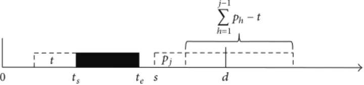
minimum cost for the 𝑗-jobs partial problem, given that the total processing time of the jobs in 𝛿₁ is 𝑡, and the earliest job in 𝛿₂ starts at time 𝑠. For 𝑗 = 1, . . . , 𝑛, 𝑡 = 0, . . . , min{𝑡_𝑠, ∑𝑗_ℎ=1𝑝_ℎ} and 𝑠 = 𝑡_𝑒, . . . , 𝑑+𝑝_𝑛−1, the recursive three-term equation is defined as (41), in which the first two terms represent the value of𝑓(𝑗, 𝑡, 𝑠) if job 𝑗 is scheduled after 𝑡_𝑒and the last term represents the value of𝑓(𝑗, 𝑡, 𝑠) if job 𝑗 is scheduled before𝑡_𝑠. From Properties 4 and 5, if𝑠 < 𝑑 then at the stage of scheduling job𝑗 in 𝛿₂two decisions should be considered: job𝑗 can be scheduled as the first job, starting at time𝑠, or as the last one, then starting at time 𝑠 + ∑𝑗−1_ℎ=1𝑝_ℎ− 𝑡. The first decision leads to the partial schedule presented in Figure 1. The cost of this partial schedule can be calculated according to

𝑓 ( 𝑗 − 1, 𝑡, 𝑠 + 𝑝_{𝑗) + 󵄨󵄨󵄨󵄨󵄨𝑠 + 𝑝𝑗− 𝑑󵄨󵄨󵄨󵄨󵄨.} (38) The second decision results in the partial schedule shown in Figure 2, and its cost is given by

𝑓 (𝑗 − 1, 𝑡, 𝑠) +󵄨󵄨󵄨󵄨󵄨󵄨󵄨󵄨 󵄨󵄨󵄨𝑠 + 𝑗 ∑ ℎ=1 𝑝_ℎ− 𝑡 − 𝑑󵄨󵄨󵄨󵄨󵄨󵄨󵄨󵄨 󵄨󵄨󵄨. (39) 0 ts te s d pj t j−1 ∑ h=1 ph− t

Figure 1: A partial schedule in𝛿₂with job𝑗 starting at time 𝑠.

0 ts te s d pj t j−1 ∑ h=1 ph− t

Figure 2: A partial schedule in𝛿₂with job𝑗 starting at time 𝑠 +

∑𝑗−1 ℎ=1𝑝ℎ− 𝑡. 0 ts te d pj t − pj · · ·

Figure 3: A partial schedule in𝛿₁with job𝑗 starting at time 𝑡_𝑠− 𝑡.

If 𝑠 ≥ 𝑑 then all jobs in 𝛿₂ are tardy, so job 𝑗 has to be scheduled as the last one in𝛿₂. As a result, in this situation the first term in recursion can be omitted.

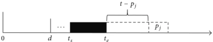
𝑓(𝑗 − 1, 𝑡 − 𝑝_𝑗, 𝑠) + 𝑑 − 𝑡_𝑠+ 𝑡 − 𝑝_𝑗is the value of𝑓(𝑗, 𝑡, 𝑠) if job𝑗 is scheduled in 𝛿₁. By Properties 3 and 4, the partial schedule in𝛿₁is constructed in a backward manner such that the last job in𝛿₁finishes exactly at time𝑡_𝑠(see Figure 3).

Initial Condition. The initial condition is

𝑓 (0, 𝑡, 𝑠) ={_{ {

0 if𝑡 = 0,

+∞ otherwise. (40)

The Recursion. The recursion is

𝑓 (𝑗, 𝑡, 𝑠) = min { { { { { { { { { { { { { 𝑓 ( 𝑗 − 1, 𝑡, 𝑠 + 𝑝𝑗) + 󵄨󵄨󵄨󵄨󵄨𝑠 + 𝑝𝑗− 𝑑󵄨󵄨󵄨󵄨󵄨, 𝑓 (𝑗 − 1, 𝑡, 𝑠) +󵄨󵄨󵄨󵄨󵄨󵄨󵄨󵄨 󵄨󵄨󵄨𝑠 + 𝑗 ∑ ℎ=1 𝑝_ℎ− 𝑡 − 𝑑󵄨󵄨󵄨󵄨󵄨󵄨󵄨󵄨 󵄨󵄨󵄨, 𝑓 ( 𝑗 − 1, 𝑡 − 𝑝_𝑗, 𝑠) + 𝑑 − 𝑡_𝑠+ 𝑡 − 𝑝_𝑗, (41) where 𝑓(𝑗 − 1, 𝑡, 𝑠 + 𝑝_𝑗) + |𝑠 + 𝑝_𝑗 − 𝑑| = 𝑓(𝑗 − 1, 𝑡, 𝑠) + |𝑠 + ∑𝑗_ℎ=1𝑝_ℎ − 𝑡 − 𝑑| = +∞ if 𝑡 > min{𝑡_𝑠, ∑𝑗−1_ℎ=1𝑝_ℎ} and 𝑓(𝑗−1, 𝑡−𝑝_𝑗, 𝑠)+𝑑−𝑡_𝑠+𝑡−𝑝_𝑗 = +∞ if 𝑡−𝑝_𝑗 < 0. The optimal objective value is equal to min_{0≤𝑡≤min{𝑡𝑠,∑}𝑛

𝑗=1𝑝𝑗}, 𝑡𝑒≤𝑠≤𝑑𝑓(𝑛, 𝑡, 𝑠).

For each state(𝑗, 𝑡, 𝑠), there are at most three operations. It follows from Property 5 that if job 1 starts after𝑑 in an optimal schedule, it must start on or before𝑑 + 𝑝_𝑛− 1, which implies that𝑠 ≤ 𝑑 + 𝑝_𝑛− 1. In addition, the value of the state variable 𝑡 is bounded by 𝑡_𝑠. Therefore, the time complexity of the algorithm is O(𝑛𝑡𝑠(𝑑 + 𝑝𝑛− 𝑡𝑒)).

0 d ts te

pj

t − pj

· · ·

Figure 4: A partial schedule in𝛿₂with job𝑗 starting at time 𝑡_𝑒+𝑡−𝑝_𝑗.

Algorithm for Case 2 (𝑡_𝑠 > 𝑑). Following the same reasoning

discussed in Case 1, let𝑓(𝑗, 𝑠, 𝑡) denote the minimum cost for the𝑗-jobs partial problem, given that the earliest job in 𝛿₁ starts at time𝑠, and the total processing time of the jobs in 𝛿₂ is𝑡. For 𝑗 = 1, . . . , 𝑛, 𝑠 = 0, . . . , min{𝑡_𝑠, 𝑑 + 𝑝_𝑛 − 1} and 𝑡 = 0, . . . , ∑𝑗_ℎ=1𝑝_ℎ, the recursive equation takes the following form.

Initial Condition. The initial condition is

𝑓 (0, 𝑠, 𝑡) ={_{ {

0 if 𝑡 = 0,

+∞ otherwise. (42)

The Recursion. The recursion is

𝑓 (𝑗, 𝑠, 𝑡) = min { { { { { { { { { { { { { 𝑓 ( 𝑗 − 1, 𝑠 + 𝑝_{𝑗, 𝑡) + 󵄨󵄨󵄨󵄨󵄨𝑠 + 𝑝𝑗− 𝑑󵄨󵄨󵄨󵄨󵄨,} 𝑓 (𝑗 − 1, 𝑠, 𝑡) +󵄨󵄨󵄨󵄨󵄨󵄨󵄨󵄨 󵄨󵄨󵄨𝑠 + 𝑗 ∑ ℎ=1 𝑝_ℎ− 𝑡 − 𝑑󵄨󵄨󵄨󵄨󵄨󵄨󵄨󵄨 󵄨󵄨󵄨, 𝑓 ( 𝑗 − 1, 𝑠, 𝑡 − 𝑝_𝑗) + 𝑡_𝑒+ 𝑡 − 𝑑, (43) where 𝑓(𝑗 − 1, 𝑠 + 𝑝_𝑗, 𝑡) + |𝑠 + 𝑝_𝑗 − 𝑑| = +∞ if 𝑠 > min{𝑡_𝑠+ 𝑡 − ∑𝑗_ℎ=1𝑝_ℎ, min{𝑡_𝑠, 𝑑 + 𝑝_𝑛− 1} − 𝑝_𝑗} or 𝑡 > ∑𝑗−1_ℎ=1𝑝_ℎ, 𝑓(𝑗−1, 𝑠, 𝑡)+|𝑠+∑𝑗_ℎ=1𝑝_ℎ−𝑡−𝑑| = +∞ if 𝑠 > 𝑡_𝑠+𝑡−∑𝑗_ℎ=1𝑝_ℎor 𝑡 > ∑𝑗−1_ℎ=1𝑝_ℎ, and𝑓(𝑗−1, 𝑠, 𝑡−𝑝_𝑗)+𝑡_𝑒+𝑡−𝑑 = +∞ if 𝑡−𝑝_𝑗 < 0. Clearly if𝑠 ≥ 𝑑, it is sufficient from Property 4 to consider that job𝑗 is scheduled either as the last one in 𝛿₁, starting at time 𝑠+∑𝑗−1_ℎ=1𝑝_ℎ−𝑡, or as the last one in 𝛿₂, then starting at time𝑡_𝑒+ 𝑡 − 𝑝_𝑗(see Figure 4). Therefore, in this situation the first term in recursion can be eliminated. The optimal objective value is found for min_{0≤𝑠≤min{𝑡𝑠,𝑑+𝑝𝑛−1}, 0≤𝑡≤∑}𝑛

𝑗=1𝑝𝑗𝑓(𝑛, 𝑠, 𝑡). Each state

(𝑗, 𝑠, 𝑡) requires at most three operations, and the state vari-ables𝑠 and 𝑡 take 𝑡_𝑠and∑𝑛_𝑗=1𝑝_𝑗as their maximum possible values, respectively. Hence, the overall time complexity of the algorithm is bounded by O(𝑛𝑡_𝑠(∑𝑛_𝑗=1𝑝_𝑗)).

Algorithm for Case 3 (𝑡_𝑠≤ 𝑑 ≤ 𝑡_𝑒). In this case, the problem is

reduced to determining the optimal assignment of the jobs to the available time windows. Once the membership in the two available time windows is specified, the optimal schedules in each available time window can be found by Properties 1, 3, and 4. Let𝑓(𝑗, 𝑡) be the minimum cost for the 𝑗-jobs partial problem, where the total processing time of the jobs in𝛿₁is𝑡. For𝑗 = 1, . . . , 𝑛 and 𝑡 = 0, . . . , min{𝑡_𝑠, ∑𝑗_ℎ=1𝑝_ℎ}, the recursive two-term equation is defined as (45), in which the first term represents the value of𝑓(𝑗, 𝑡) if job 𝑗 is scheduled in 𝛿₁and the

second term represents the value of𝑓(𝑗, 𝑡) if job 𝑗 is scheduled in𝛿₂.

Initial Condition. The initial condition is

𝑓 (0, 𝑡) ={_{ {

0 if 𝑡 = 0,

+∞ otherwise. (44)

The Recursion. The recursion is

𝑓 (𝑗, 𝑡) = min { { { { { { { 𝑓 ( 𝑗 − 1, 𝑡 − 𝑝_𝑗) + 𝑑 − 𝑡_𝑠+ 𝑡 − 𝑝_𝑗, 𝑓 (𝑗 − 1, 𝑡) + 𝑡_𝑒+∑𝑗 ℎ=1 𝑝_ℎ− 𝑡 − 𝑑, (45) where𝑓(𝑗 − 1, 𝑡 − 𝑝_𝑗) + 𝑑 − 𝑡_𝑠+ 𝑡 − 𝑝_𝑗= +∞ if 𝑡 − 𝑝_𝑗< 0 and 𝑓(𝑗−1, 𝑡)+𝑡_𝑒+∑𝑗_ℎ=1𝑝_ℎ−𝑡−𝑑 = +∞ if 𝑡 > min{𝑡_𝑠, ∑𝑗−1_ℎ=1𝑝_ℎ}. The optimal objective value is equal to min_{0≤𝑡≤min{𝑡𝑠,∑}𝑛

𝑗=1𝑝𝑗}𝑓(𝑛, 𝑡).

As described above, it can be established that the algorithm finds an optimal schedule in O(𝑛𝑡𝑠) time.

5. Experimental Results

In this section, the numerical results are provided to assess the performance of the different methods presented above. The dynamic programming algorithms were written in C++ language and the mixed integer linear programs were solved by ILOG CPLEX 12.4. The experiments were conducted on a PC with a 3.4 GHz processor and 4 GB RAM.

5.1. Comparison between the Proposed Methods. Here, the

computation times (in CPU seconds) and the optimality gaps of the proposed methods are compared. The problem instances were generated as follows:

(1) The number of jobs was chosen from 5 to 200. (2) The job processing times followed the discrete

uni-form distribution [1, 𝑝_max= 10].

(3) The start time of the unavailability interval was set at ⌊𝑃 ∑𝑛_𝑗=1𝑝_𝑗⌋ with the proportionality coefficient 𝑃 ∈ {0.25, 0.5, 0.75}. For simplicity, the duration of the unavailability interval was set to be⌊𝑝 = (∑𝑛_𝑗=1𝑝_𝑗)/𝑛⌋. The integer due date was generated uniformly as follows. Case 1 (𝑡_𝑒< 𝑑). Consider 𝑑 ∈ [𝑡_𝑒+∑ 𝑛 𝑗=1𝑝𝑗 3 (1 − 𝑅) , 𝑡𝑒+ ∑𝑛_𝑗=1𝑝_𝑗 3 (1 + 𝑅)] . (46) Case 2 (𝑡_𝑠> 𝑑). Consider 𝑑 ∈ [𝑡𝑠 2 (1 − 𝑅) , 𝑡_𝑠 2 (1 + 𝑅)] . (47) Case 3 (𝑡_𝑠≤ 𝑑 ≤ 𝑡_𝑒). Consider 𝑑 ∈ [𝑡𝑠+ 𝑡𝑒− 𝑅𝑝 2 , 𝑡_𝑠+ 𝑡_𝑒+ 𝑅𝑝 2 ] , (48)

Table 1: Comparison between the exact methods.

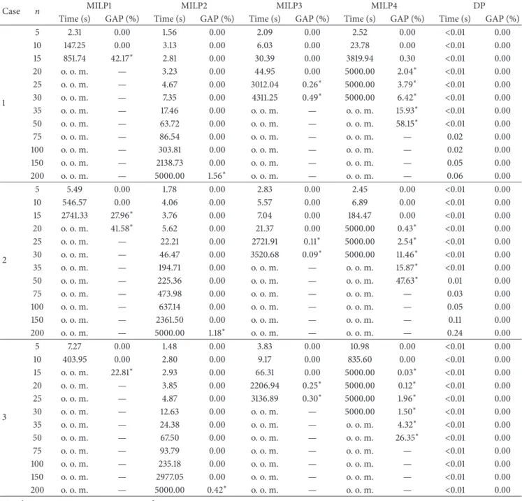
Case n MILP1 MILP2 MILP3 MILP4 DP

Time (s) GAP (%) Time (s) GAP (%) Time (s) GAP (%) Time (s) GAP (%) Time (s) GAP (%)

1 5 2.31 0.00 1.56 0.00 2.09 0.00 2.52 0.00 <0.01 0.00 10 147.25 0.00 3.13 0.00 6.03 0.00 23.78 0.00 <0.01 0.00 15 851.74 42.17∗ 2.81 0.00 30.39 0.00 3819.94 0.30 <0.01 0.00 20 o. o. m. — 3.23 0.00 44.95 0.00 5000.00 2.04∗ <0.01 0.00 25 o. o. m. — 4.67 0.00 3012.04 0.26∗ 5000.00 3.79∗ <0.01 0.00 30 o. o. m. — 7.35 0.00 4311.25 0.49∗ 5000.00 6.42∗ <0.01 0.00 35 o. o. m. — 17.46 0.00 o. o. m. — o. o. m. 15.93∗ <0.01 0.00 50 o. o. m. — 63.72 0.00 o. o. m. — o. o. m. 58.15∗ <0.01 0.00 75 o. o. m. — 86.54 0.00 o. o. m. — o. o. m. — 0.02 0.00 100 o. o. m. — 303.81 0.00 o. o. m. — o. o. m. — 0.02 0.00 150 o. o. m. — 2138.73 0.00 o. o. m. — o. o. m. — 0.05 0.00 200 o. o. m. — 5000.00 1.56∗ o. o. m. — o. o. m. — 0.06 0.00 2 5 5.49 0.00 1.78 0.00 2.83 0.00 2.45 0.00 <0.01 0.00 10 546.57 0.00 4.06 0.00 5.57 0.00 6.89 0.00 <0.01 0.00 15 2741.33 27.96∗ 3.76 0.00 7.04 0.00 184.47 0.00 <0.01 0.00 20 o. o. m. 41.58∗ 5.62 0.00 21.37 0.00 5000.00 0.43∗ <0.01 0.00 25 o. o. m. — 22.21 0.00 2721.91 0.11∗ 5000.00 2.54∗ <0.01 0.00 30 o. o. m. — 46.47 0.00 3520.68 0.09∗ 5000.00 11.46∗ <0.01 0.00 35 o. o. m. — 194.71 0.00 o. o. m. — o. o. m. 15.87∗ <0.01 0.00 50 o. o. m. — 225.36 0.00 o. o. m. — o. o. m. 47.63∗ 0.01 0.00 75 o. o. m. — 473.98 0.00 o. o. m. — o. o. m. — 0.03 0.00 100 o. o. m. — 637.14 0.00 o. o. m. — o. o. m. — 0.05 0.00 150 o. o. m. — 2361.50 0.00 o. o. m. — o. o. m. — 0.11 0.00 200 o. o. m. — 5000.00 1.18∗ o. o. m. — o. o. m. — 0.24 0.00 3 5 7.27 0.00 1.48 0.00 3.83 0.00 10.98 0.00 <0.01 0.00 10 403.95 0.00 2.80 0.00 9.17 0.00 835.60 0.00 <0.01 0.00 15 o. o. m. 22.81∗ 2.93 0.00 66.31 0.00 5000.00 0.03∗ <0.01 0.00 20 o. o. m. — 3.85 0.00 2206.94 0.25∗ 5000.00 0.12∗ <0.01 0.00 25 o. o. m. — 4.87 0.00 3136.89 0.30∗ 5000.00 1.96∗ <0.01 0.00 30 o. o. m. — 12.63 0.00 o. o. m. — 5000.00 1.50∗ <0.01 0.00 35 o. o. m. — 24.38 0.00 o. o. m. — o. o. m. 4.32∗ <0.01 0.00 50 o. o. m. — 67.50 0.00 o. o. m. — o. o. m. 26.35∗ <0.01 0.00 75 o. o. m. — 93.79 0.00 o. o. m. — o. o. m. — <0.01 0.00 100 o. o. m. — 235.18 0.00 o. o. m. — o. o. m. — <0.01 0.00 150 o. o. m. — 2977.05 0.00 o. o. m. — o. o. m. — <0.01 0.00 200 o. o. m. — 5000.00 0.42∗ o. o. m. — o. o. m. — <0.01 0.00

DP = dynamic programming; o. o. m. = out of memory.

of which the due date factor was chosen from 𝑅 ∈ {0.3, 0.5, 0.7}.

For each case, 10 instances were randomly generated for each problem size. The results of this experiment are summarized in Table 1. The symbol “—” denotes the cases that no feasible solution found within a time limit 5000 seconds or the program is interrupted due to lack of memory. The symbol “∗” denotes that the optimality gap is calculated as [(𝐶(IB) − optimum)/optimum] × 100%, where 𝐶(IB)

is the incumbent solution obtained before the program is terminated.

According to these results, it is clear that MILP2 and the dynamic programming method are much more effective than the other mixed integer linear programming formulations. MILP2 was able to handle the problems with close to 150 jobs, while it was difficult to use the latter approaches to solve instances with more than 20 jobs. However, the obtained results corroborate the findings in Kacem et al. [44] that the dynamic programming method could be superior to other

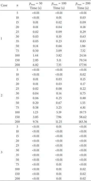
Table 2: Dynamic programming method performance.

Case n 𝑝max= 50 𝑝max= 100 𝑝max= 200

Time (s) Time (s) Time (s)

1 5 <0.01 <0.01 <0.01 10 <0.01 0.01 0.03 15 0.01 0.02 0.09 20 0.01 0.04 0.18 25 0.02 0.09 0.29 30 0.03 0.10 0.63 35 0.05 0.23 0.83 50 0.14 0.66 1.86 75 0.50 3.09 7.32 100 1.44 3.82 24.16 150 2.85 5.11 70.54 200 6.82 7.35 177.91 2 5 <0.01 <0.01 <0.01 10 <0.01 <0.01 0.02 15 0.01 0.03 0.15 20 0.01 0.03 0.17 25 0.02 0.08 0.22 30 0.04 0.14 0.75 35 0.06 0.25 0.88 50 0.20 0.67 1.55 75 0.58 3.25 6.81 100 1.23 5.19 19.73 150 3.85 7.96 58.62 200 9.76 11.25 183.36 3 5 <0.01 0.01 <0.01 10 <0.01 <0.01 <0.01 15 <0.01 <0.01 <0.01 20 <0.01 <0.01 <0.01 25 <0.01 <0.01 <0.01 30 <0.01 <0.01 <0.01 35 <0.01 <0.01 <0.01 50 <0.01 <0.01 <0.01 75 <0.01 0.01 <0.01 100 <0.01 0.01 0.02 150 <0.01 0.01 0.02 200 <0.01 0.01 0.02

methods. As compared to MILP2, the dynamic programming method was more efficient in attaining the optimal schedules and no problems due to memory requirement. In addition, the superiority of the dynamic programming method became more significant as the problem size increased.

The dynamic programming method is complex. So, we add particularly further experiments with𝑝_max = 50, 100, and 200 to evaluate the impact of the length of the scheduling horizon on the method. Table 2 presents computation times required to obtain the optimal solutions for each case. As the results show, the dynamic programming method became relatively expensive, in terms of CPU time, when the value of∑𝑛_𝑗=1𝑝_𝑗 increased. Moreover, as compared to the results

of the mixed integer linear programming methods for the problems with𝑝_max= 10, the dynamic programming method was still capable of quickly solving problems with hundreds of jobs. Given the above observations, we can conclude that the dynamic programming method may be more promising for the addressed problem.

5.2. Dynamic Programming Method Experiments. In this

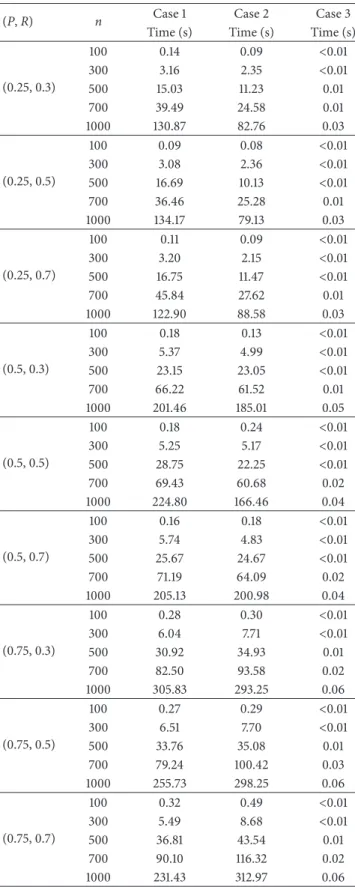
section, the influence of the proportionality coefficient𝑃 and the due date factor𝑅 on the performance of the dynamic programming method is analyzed. The number of jobs varied in 𝑛 ∈ {100, 300, 500, 700, 1000}, and the job processing times followed a discrete uniform distribution defined by the interval [1, 20]. The due date, start time, and the duration of the unavailability interval were set as those described in the previous experiment. For each treble (𝑛, 𝑃, 𝑅), 10 instances were randomly generated. Hence, this experiment contains a total of 450 instances for each case. For Cases 1 and 2, it can be observed from Table 3 that for the same problem sizes the average of CPU times became higher when the value of 𝑃 increased. The results also indicate that as compared to Case 1 when𝑃 was small (≤ 0.5) the problems of Case 2 were relatively easy to solve. Nevertheless, it is noticed that the variation of 𝑅 did not have a significant influence on the problem hardness. With respect to Case 3, the results indicate that for the same problem sizes the larger the value of𝑃 was the harder the problems became. It seems that the value of𝑅 had no effect on the performance of this method. Indeed, in this case the algorithm is implemented in O(𝑛𝑡_𝑠) time and therefore, its complexity is independent of the due date setting.

6. Conclusions

This paper addresses the single-machine scheduling problem to minimize the TET in relation to a common due date, where the machine is subject to a given unavailability interval during which the production is not allowed. To the best of our knowledge, no exact algorithms have previously been published for this problem. Therefore, this study proposes solution methodologies and properties of an optimal sched-ule for the purpose of exposing insights that may ultimately be useful in research on more complicated models.

First, four mixed integer linear programming formu-lations with different types of binary variables that seize the scheduling decisions are introduced. Observing that these formulations are time-consuming to derive an optimal solution with the increase of the number of jobs, a dynamic programming method based on the solution properties is then proposed to deal with large-scale problems. Numerical results for problems with up to 1000 jobs demonstrate that the dynamic programming method is well suited to finding optimal schedules in comparison with the mixed integer linear programming methods and its advantage gets bigger as the problems size increases. In summary, when the complexity of the dynamic programming method remains correct, it is very promising for practical problems.

Table 3: Influence of the proportionality coefficient𝑃 and the due

date factor𝑅 on the dynamic programming method.

(P, R) n Case 1 Case 2 Case 3

Time (s) Time (s) Time (s)

(0.25, 0.3) 100 0.14 0.09 <0.01 300 3.16 2.35 <0.01 500 15.03 11.23 0.01 700 39.49 24.58 0.01 1000 130.87 82.76 0.03 (0.25, 0.5) 100 0.09 0.08 <0.01 300 3.08 2.36 <0.01 500 16.69 10.13 <0.01 700 36.46 25.28 0.01 1000 134.17 79.13 0.03 (0.25, 0.7) 100 0.11 0.09 <0.01 300 3.20 2.15 <0.01 500 16.75 11.47 <0.01 700 45.84 27.62 0.01 1000 122.90 88.58 0.03 (0.5, 0.3) 100 0.18 0.13 <0.01 300 5.37 4.99 <0.01 500 23.15 23.05 <0.01 700 66.22 61.52 0.01 1000 201.46 185.01 0.05 (0.5, 0.5) 100 0.18 0.24 <0.01 300 5.25 5.17 <0.01 500 28.75 22.25 <0.01 700 69.43 60.68 0.02 1000 224.80 166.46 0.04 (0.5, 0.7) 100 0.16 0.18 <0.01 300 5.74 4.83 <0.01 500 25.67 24.67 <0.01 700 71.19 64.09 0.02 1000 205.13 200.98 0.04 (0.75, 0.3) 100 0.28 0.30 <0.01 300 6.04 7.71 <0.01 500 30.92 34.93 0.01 700 82.50 93.58 0.02 1000 305.83 293.25 0.06 (0.75, 0.5) 100 0.27 0.29 <0.01 300 6.51 7.70 <0.01 500 33.76 35.08 0.01 700 79.24 100.42 0.03 1000 255.73 298.25 0.06 (0.75, 0.7) 100 0.32 0.49 <0.01 300 5.49 8.68 <0.01 500 36.81 43.54 0.01 700 90.10 116.32 0.02 1000 231.43 312.97 0.06

Although the computational complexity associated with the mixed integer linear programming formulations makes it usually difficult for optimization software that addresses

industrial-dimensioned problems in reasonable solution time, the mixed integer linear programming methods are useful to understand the structure of the problem and may be the better algorithmic choice when convenience in imple-mentation is considered. Further research will be devoted to deriving of valid inequalities and investigation of the development of tighter upper bounds for the total processing time in each available time window in order to improve the computational efficiency of the proposed methods. It might be interesting to extend our schemes to the problem with multiple unavailability intervals.

Competing Interests

The authors declare that there are no competing interests regarding the publication of this paper.

References

[1] K. R. Baker and G. D. Scudder, “Sequencing with earliness and tardiness penalties: a review,” Operations Research, vol. 38, no. 1, pp. 22–36, 1990.

[2] D. Biskup and M. Feldmann, “Benchmarks for scheduling on a single machine against restrictive and unrestrictive common due dates,” Computers and Operations Research, vol. 28, no. 8, pp. 787–801, 2001.

[3] V. Gordon, J.-M. Proth, and C. Chu, “A survey of the state-of-the-art of common due date assignment and scheduling research,” European Journal of Operational Research, vol. 139, no. 1, pp. 1–25, 2002.

[4] V. Lauff and F. Werner, “Scheduling with common due date, earliness and tardiness penalties for multimachine problems: a survey,” Mathematical and Computer Modelling, vol. 40, no. 5-6, pp. 637–655, 2004.

[5] J. J. Kanet, “Minimizing the average deviation of job completion times about a common due date,” Naval Research Logistics Quarterly, vol. 28, no. 4, pp. 643–651, 1981.

[6] U. Bagchi, R. S. Sullivan, and Y.-L. Chang, “Minimizing mean absolute deviation of completion times about a common due date,” Naval Research Logistics Quarterly, vol. 33, no. 2, pp. 227– 240, 1986.

[7] P. S. Sundararaghavan and M. U. Ahmed, “Minimizing the sum of absolute lateness in single-machine and multimachine scheduling,” Naval Research Logistics Quarterly, vol. 31, no. 2, pp. 325–333, 1984.

[8] H. Emmons, “Scheduling to a common due date on parallel uniform processors,” Naval Research Logistics, vol. 34, no. 6, pp. 803–810, 1987.

[9] N. G. Hall, W. Kubiak, and S. P. Sethi, “Earliness-tardiness scheduling problems, II: deviation of completion times about a restrictive common due date,” Operations Research, vol. 39, no. 5, pp. 847–856, 1991.

[10] J. A. Hoogeveen and S. L. van de Velde, “Scheduling around a small common due date,” European Journal of Operational Research, vol. 55, no. 2, pp. 237–242, 1991.

[11] J. A. Hoogeveen, H. Oosterhout, and S. L. van de Velde, “New lower and upper bounds for scheduling around a small common due date,” Operations Research, vol. 42, no. 1, pp. 102–110, 1994.

[12] W. Szwarc, “Single-machine scheduling to minimize absolute deviation of completion times from a common due date,” Naval Research Logistics, vol. 36, no. 5, pp. 663–673, 1989.

[13] J. A. Ventura and M. X. Weng, “An improved dynamic program-ming algorithm for the single-machine mean absolute deviation problem with a restrictive common due date,” Operations Research Letters, vol. 17, no. 3, pp. 149–152, 1995.

[14] H. Sarper, “Minimizing the sum of absolute deviations about a common due date for the two-machine flow shop problem,” Applied Mathematical Modelling, vol. 19, no. 3, pp. 153–161, 1995. [15] C. S. Sakuraba, D. P. Ronconi, and F. Sourd, “Scheduling in a two-machine flowshop for the minimization of the mean absolute deviation from a common due date,” Computers & Operations Research, vol. 36, no. 1, pp. 60–72, 2009.

[16] C. S. Sung and J. I. Min, “Scheduling in a two-machine flow-shop with batch processing machine(s) for earliness/tardiness measure under a common due date,” European Journal of Operational Research, vol. 131, no. 1, pp. 95–106, 2001.

[17] W. K. Yeung, C. O˘guz, and T. C. E. Cheng, “Two-stage flowshop earliness and tardiness machine scheduling involving a common due window,” International Journal of Production Economics, vol. 90, no. 3, pp. 421–434, 2004.

[18] V. Lauff and F. Werner, “On the complexity and some properties of multi-stage scheduling problems with earliness and tardiness penalties,” Computers & Operations Research, vol. 31, no. 3, pp. 317–345, 2004.

[19] C.-Y. Lee, L. Lei, and M. Pinedo, “Current trends in determinis-tic scheduling,” Annals of Operations Research, vol. 70, pp. 1–41, 1997.

[20] G. Schmidt, “Scheduling with limited machine availability,” European Journal of Operational Research, vol. 121, no. 1, pp. 1–15, 2000.

[21] Y. Ma, C. Chu, and C. Zuo, “A survey of scheduling with deterministic machine availability constraints,” Computers and Industrial Engineering, vol. 58, no. 2, pp. 199–211, 2010. [22] C. Low, M. Ji, C.-J. Hsu, and C.-T. Su, “Minimizing the

makespan in a single machine scheduling problems with flexible and periodic maintenance,” Applied Mathematical Modelling, vol. 34, no. 2, pp. 334–342, 2010.

[23] G. Mosheiov and J. B. Sidney, “Scheduling a deteriorating maintenance activity on a single machine,” Journal of the Operational Research Society, vol. 61, no. 5, pp. 882–887, 2010. [24] C.-l. Zhao and H.-Y. Tang, “Single machine scheduling with

general job-dependent aging effect and maintenance activities to minimize makespan,” Applied Mathematical Modelling, vol. 34, no. 3, pp. 837–841, 2010.

[25] F. ´Angel-Bello, A. ´Alvarez, J. Pacheco, and I. Mart´ınez, “A

single machine scheduling problem with availability constraints and sequence-dependent setup costs,” Applied Mathematical Modelling, vol. 35, no. 4, pp. 2041–2050, 2011.

[26] Y. Huo and H. Zhao, “Bicriteria scheduling concerned with makespan and total completion time subject to machine avail-ability constraints,” Theoretical Computer Science, vol. 412, no. 12-14, pp. 1081–1091, 2011.

[27] S.-L. Yang, Y. Ma, D.-L. Xu, and J.-B. Yang, “Minimizing total completion time on a single machine with a flexible maintenance activity,” Computers and Operations Research, vol. 38, no. 4, pp. 755–770, 2011.

[28] J.-Y. Lee and Y.-D. Kim, “Minimizing the number of tardy jobs in a single-machine scheduling problem with periodic

maintenance,” Computers & Operations Research, vol. 39, no. 9, pp. 2196–2205, 2012.

[29] Y. Yin, T. C. E. Cheng, D. Xu, and C.-C. Wu, “Common due date assignment and scheduling with a rate-modifying activity to minimize the due date, earliness, tardiness, holding, and batch delivery cost,” Computers and Industrial Engineering, vol. 63, no. 1, pp. 223–234, 2012.

[30] M. Dong, “Parallel machine scheduling with limited control-lable machine availability,” International Journal of Production Research, vol. 51, no. 8, pp. 2240–2252, 2013.

[31] C.-J. Hsu, M. Ji, J.-Y. Guo, and D.-L. Yang, “Unrelated parallel-machine scheduling problems with aging effects and deteriorat-ing maintenance activities,” Information Sciences, vol. 253, pp. 163–169, 2013.

[32] L. Shen, D. Wang, and X.-Y. Wang, “Parallel-machine schedul-ing with non-simultaneous machine available time,” Applied Mathematical Modelling, vol. 37, no. 7, pp. 5227–5232, 2013. [33] B. Vahedi-Nouri, P. Fattahi, M. Rohaninejad, and R.

Tavakkoli-Moghaddam, “Minimizing the total completion time on a single machine with the learning effect and multiple availability constraints,” Applied Mathematical Modelling, vol. 37, no. 5, pp. 3126–3137, 2013.

[34] D. Xu and D.-L. Yang, “Makespan minimization for two parallel machines scheduling with a periodic availability constraint: mathematical programming model, average-case analysis, and anomalies,” Applied Mathematical Modelling, vol. 37, no. 14-15, pp. 7561–7567, 2013.

[35] N. Hashemian, C. Diallo, and B. Vizv´ari, “Makespan minimiza-tion for parallel machines scheduling with multiple availability constraints,” Annals of Operations Research, vol. 213, no. 1, pp. 173–186, 2014.

[36] V. Kaplano˘glu, “Multi-agent based approach for single machine scheduling with sequence-dependent setup times and machine maintenance,” Applied Soft Computing, vol. 23, pp. 165–179, 2014.

[37] K. Rustogi and V. A. Strusevich, “Combining time and position dependent effects on a single machine subject to rate-modifying activities,” Omega, vol. 42, no. 1, pp. 166–178, 2014.

[38] Y. Yin, D. Ye, and G. Zhang, “Single machine batch scheduling to minimize the sum of total flow time and batch delivery cost with an unavailability interval,” Information Sciences, vol. 274, pp. 310–322, 2014.

[39] Y. Yin, W.-H. Wu, T. C. E. Cheng, and C.-C. Wu, “Due-date assignment and single-machine scheduling with generalised position-dependent deteriorating jobs and deteriorating multi-maintenance activities,” International Journal of Production Research, vol. 52, no. 8, pp. 2311–2326, 2014.

[40] K. Rustogi and V. A. Strusevich, “Single machine scheduling with time-dependent linear deterioration and rate-modifying maintenance,” Journal of the Operational Research Society, vol. 66, no. 3, pp. 500–515, 2015.

[41] C. Low, R.-K. Li, G.-H. Wu, and C.-L. Huang, “Minimizing the sum of absolute deviations under a common due date for a single-machine scheduling problem with availability constraints,” Journal of Industrial and Production Engineering, vol. 32, no. 3, pp. 204–217, 2015.

[42] R. L. Graham, E. L. Lawler, J. K. Lenstra, and A. H. G. R. Kan, “Optimization and approximation in deterministic sequencing and scheduling: a survey,” Annals of Discrete Mathematics, vol. 5, pp. 287–326, 1979.

[43] T. C. E. Cheng and H. G. Kahlbacher, “A proof for the longest-job-first policy in one-machine scheduling,” Naval Research Logistics, vol. 38, no. 5, pp. 715–720, 1991.

[44] I. Kacem, C. Chu, and A. Souissi, “Single-machine scheduling with an availability constraint to minimize the weighted sum of the completion times,” Computers & Operations Research, vol. 35, no. 3, pp. 827–844, 2008.

Submit your manuscripts at

http://www.hindawi.com

Hindawi Publishing Corporation

http://www.hindawi.com Volume 2014

Mathematics

Hindawi Publishing Corporation

http://www.hindawi.com Volume 2014 Mathematical Problems in Engineering

Hindawi Publishing Corporation http://www.hindawi.com

Differential Equations International Journal of

Volume 2014

Hindawi Publishing Corporation

http://www.hindawi.com Volume 2014 Hindawi Publishing Corporationhttp://www.hindawi.com Volume 2014

Hindawi Publishing Corporation

http://www.hindawi.com Volume 2014 Mathematical PhysicsAdvances in

Complex Analysis

Hindawi Publishing Corporation

http://www.hindawi.com Volume 2014

Optimization

Hindawi Publishing Corporation

http://www.hindawi.com Volume 2014

Combinatorics

Hindawi Publishing Corporation

http://www.hindawi.com Volume 2014

International Journal of

Hindawi Publishing Corporation

http://www.hindawi.com Volume 2014

Journal of Hindawi Publishing Corporation

http://www.hindawi.com Volume 2014

Function Spaces

Abstract and Applied Analysis

Hindawi Publishing Corporation

http://www.hindawi.com Volume 2014 International Journal of Mathematics and Mathematical Sciences

Hindawi Publishing Corporation http://www.hindawi.com Volume 2014

The Scientific

World Journal

Hindawi Publishing Corporation

http://www.hindawi.com Volume 2014

Hindawi Publishing Corporation

http://www.hindawi.com Volume 2014

Discrete Dynamics in Nature and Society Hindawi Publishing Corporation

http://www.hindawi.com Volume 2014

Hindawi Publishing Corporation

http://www.hindawi.com Volume 2014

Discrete Mathematics

Hindawi Publishing Corporation

http://www.hindawi.com Volume 2014 Hindawi Publishing Corporationhttp://www.hindawi.com Volume 2014

Stochastic Analysis