ADAPTIVE-CONTROL OPTIMIZATION IN END MILLING USING NEURAL NETWORKS

(1)

~

Pergamon

A D A P T I V E C O N T R O L O P T I M I Z A T I O N I N E N D M I L L I N G U S I N G N E U R A L N E T W O R K S

SmuH-TARN6 CHIANG,t DIN6-I LIV,t AN-CHEN LEES" and WEI-HUA CmENGt

(Received 6 August 1993)

A b s t r a c t - - I n this paper, we propose an architecture with two different kinds of neural networks for on-line determination of optimal cutting conditions. A back-propagation network with three inputs and four o u t p u t s is used to m o d e l the cutting process. A second network, which parallelizes the a u g m e n t e d Lagrange multiplier algorithm, d e t e r m i n e s the c o r r e s p o n d i n g optimal cutting p a r a m e t e r s by maximizing the material removal rate according to appropriate operating constraints. D u e to its parallelism, this architecture can greatly reduce processing time a n d m a k e real-time control possible. Numerical simulations and a series of e x p e r i m e n t s are conducted on e n d milling to confirm the feasibility of this architecture.

1. I N T R O D U C T I O N

THE USE OF COMPUTER numerical control (CNC) systems has grown tremendously in recent decades. However, a remaining drawback of these systems is that the operating parameters, such as feedrate, speed, and depth of cut, are programmed off-line and the selection of these parameters is based on the part programmer's experience and knowledge. To prevent damage to the cutting tool, the operating conditions are usually set extremely conservatively. As a result, many CNC systems are inefficient and run under the operating conditions that are far from the optimal criteria.

For this reason, adaptive control, which provides on-line adjustment of the operating parameters, is being studied with interest. Adaptive control systems can be classified into two types [1]: (1)adaptive control with optimization (ACO) and (2)adaptive control with constraints (ACC). In ACO systems, the controller adjusts the operating parameters to maximize a given performance index under various constraints. In ACC systems, on the other hand, the operating parameters are adjusted to regulate one or more output parameters (typically cutting force or cutting power) to their limit values. In fact, the objective of most ACC systems is also to increase a given performance index by assuming that the optimal solution occurs on a constraint boundary.

Since machining is a time-varying process, most adaptive control methods [2] apply the recursive least squares method to in-process estimate the parameters of the special empirical formula or the linearized model. However, in many cases, no reliable model is available or the reduced linearized model is not accurate enough to depict the input/output (I/O) relationship of the cutting process. Furthermore, as more cutting constraints are taken into account, the computing time for these methods increases, because more parameters must be estimated. Therefore, neural networks, which can map the I/O relationship and possesses massive parallel computing capability, have attracted much attention in research on machining processes.

Chryssolouris and Guillot [3] modeled the machining process by a multiple regression method and a neural network and concluded that neural networks are superior to conventional multiple regression methods. Madey et al. [4] had a neural network learn the I/O relationship of a human operator's actions. The neural network could then work like the operator. However, this method is limited to the trained cutting conditions. Rangwala and Dornfeld [5] presented a scheme that used a multilayered

t D e p a r t m e n t of Mechanical E n g i n e e r i n g , National Chiao T u n g University, 1001 Ta H s u e h R o a d , H s i n c h u 300, Taiwan, R . O . C .

637

(2)

638 SHIUH-TARNG CHIANG et al.

perceptron neural network to model the turning process and an augmented Lagrange multiplier (ALM) method to optimize the material removal rate. They presented only a computer simulation. Later, Choi et al. [6] experimented with this scheme on a turning process, but employed a different optimum strategy, the barrier function (one of the sequential unconstrained minimization techniques). Since the calculation for optimization takes a great deal of time, their scheme was unable to reduce the error level between the neural network and actual lathe immediately. Thus this method may result in a false optimal result.

Although neural networks can represent more I/O relationships without increasing computing time, the networks employed in all of the previous work in this area require a great deal of time to find the optimal cutting conditions. Thus the calculated optimal conditions are far from the real optimal conditions. More recently, a special type of neural network that parallelizes the optimal algorithm has been used to solve on-line optimization problems [7].

Tank and Hopfield [8] first found that a neural network can seek to minimize the energy function and designed a neural network for finding a function minimum. Chua and Lin [9] used integrator cells to model neurons and mapped the cost function and constraints into a canonical nonlinear circuit based on the Kuhn-Tucker conditions. Kennedy and Chua [10] showed that the linear programming circuit of Tank and Hopfield [8], after some modification, can be reduced to the circuit of Chua and Lin [9]. Rodriguez-Vazquez et al. [11] replaced the RC-active technique by an SC-reactive technique, which is more suitable for VLSI implementation. Most of the above networks use the penalty method to solve optimization problems. However, Cichocki and Unbe- hauen [12] proposed a structure similar to Rodriguez-Vazquez et al.'s [11], that, unlike his, employed an ALM method. Their structure parallelizes existing optimal algorithms and constitutes a parallel network. Because of their parallelism, these networks make on-line optimization possible.

In this paper, a neural network based adaptive control with optimization (NNBACO) system that includes two different kinds of neural networks is proposed for on-line selection of optimal cutting parameters and control of the machining process. A back- propagation network with three inputs and four outputs is used as a general-purpose model to learn the end milling. A second network, which parallelizes the ALM method, finds the corresponding optimal cutting conditions based on the cost function and maximum material removal rate ( M R R ) , subject to certain constraints. Owing to the parallel processing ability of this architecture, the processing time will not increase when more constraints are added. Numerical simulations and a set of experiments that apply this N N B A C O system on end milling are presented to demonstrate its capabilities. These results show that this system is valid within the cutting conditions examined.

This paper is organized as follows. Section 2 gives an overview of neural networks. Section 3 first presents the circuit used for solving on-line optimization of a cutting process and then describes the architecture of the proposed NNBACO system. Section 4 presents a simulation that illustrates the application of the proposed structure in end milling. Section 5 describes the experimental procedure and results. Conclusions are given in the last section.

2. N E U R A L NETWORKS

In an artificial neural network, the unit analogous to the biological neuron is referred to as a "processing element" (PE) (see Fig. 1). Like a biological nervous system, an artificial neural network consists of a large number of interconnected PEs. A P E has many inputs oj.~_~, but only a single output o~.~, which can fan out to many other PEs in the network. The basic function of a neuron is to sum its inputs and to produce an output. Let wi4.~ be the weight between the ith input branch in the kth layer connected to the jth neuron in the (k - 1) layer. Then the output of the ith neuron oi,k is given by

(3)

Adaptive Control Optimization 639 O 1,k-I W -'-- y , i i ~ N ~ W ; I L" . - o 2,k-1 ~ nat I f w 0 " z Wi,j, k j,k-1

FI~. 1. Schematic diagram of the basic model.

1

(1)

where f(.) is called the activation function.

The operation of neural networks can be divided into two main phases: learning and recall. Learning is the process of adapting the weights in response to stimuli at the inputs. Once the weights have been adapted, the neural network has learned the I/O mapping. Recall refers to how the network processes a stimulus presented at the input and creates a response at the output.

Many kinds of neural network models have been proposed in recent years. A supervised processing neural network, back-propagation, is introduced in the following. The back-propagation network, shown in Fig. 2, was introduced by Rumelhart and McClelland [13] in 1986. A typical back-propagation network is a supervised multilayer network that includes an input layer, an output layer, and at least one hidden layer and in which each layer is fully connected to the succeeding layer.

As illustrated by the solid lines in Fig. 2, the stimuli are fed into the input layer and propagated forward to the output layer. The output is compared with the desired one and then the error signal is propagated backward through the network, as shown by the dashed lines, to upgrade the weights of each layer. The name back-propagation is derived from the backward propagation of the error signal.

The main steps in the back-propagation algorithm are summarized as follows: STEP 1 Initialize all weights wij.k with small random values.

STEP 2 Present input patterns and specify the corresponding desired outputs. STEP 3 Calculate the actual outputs of all the nodes, using the present value of the

weights, by Oi.k = f ( n e t i . k ) (2) where neti.k = ~ [Wij.k " O j . k - l ] . (3) J Output layer Hidden layer Input layer

(4)

STEP 4 Find an error term 8i for an output node using the equation

8 i . k = ( d i - O i . k ) • f ( n e t i . k ) .

For a hidden layer node, find the error term using the equation

(4)

8i.k = f ( n e t j . k _ , ) • ~ [S,.k+, • W,.i.k+,] (5)

l

where l is the number of neurons in the layer above node j. STEP 5 Adjust the weights by

w ( k + 1) = w ( k ) + ~ • 8Ok • O,.k + 13 " ( w ( k ) - w ( k - 1)) , (6)

where rl is the learning rate and 13 is a constant, between 0 and 1, which determines the effect of past weight change on the current direction of move- ment in the weight space.

STEP 6 Present another input and go back to STEP 2 cyclically until all the weights converge.

Since neural networks have a highly parallel structure, they are well suited to parallel implementation. Such an implementation can result in very fast processing and can achieve a very high degree of fault tolerance. In addition, since neural networks can naturally process many inputs and have many outputs, they are readily applicable to multivariable systems. Because of these promising features, recently neural networks have been widely applied in fields such as image compression, character recognition, and automatic control [14]. Moreover, specially designed chips for neural networks have also been developed.

3. N E U R A L N E T W O R K BASED A D A P T I V E C O N T R O L WITH O P T I M I Z A T I O N IN END MILLING

In what follows, the mathematical formulation for optimization of cutting conditions is described and the parallel structure used for solving the on-line optimization problem of a cutting process is developed. The neural network based adaptive control with optimization ( N N B A C O ) system applied to the end milling process is proposed in the last subsection.

3.1. Mathematical formulation for optimization o f cutting conditions

In a cutting process, in order to prevent damage to the cutting tool and maintain the minimum acceptable workpiece surface finish, there are upper bounds on the cutting forces in the X and Y directions (Fx,Fv), the power (P), and the surface finish (Ra). Similarly, because of the variety of cutting tools used and variations in machine capacity, the input variables (feedrate per tooth (ft), axial depth of cut (Ao) and radial depth of cut (Rd)) also have their own operating ranges. Although there are many factors that restrict the operating conditions, a high material removal rate is also required. Hence, the above description can be transformed into an optimization problem: under the limitations on the inputs and outputs, find a set of optimal inputs that will maximize the MRR, i.e.

maximize the performance index

F = f t " Ad " Ro (7)

subject to the following constraints on the input variables:

Min. offt - f t - Max. offt Min. of Rd --< Ro - Max. of Rd

(5)

Adaptive Control Optimization 641

and the following constraints on the output variables:

Fx - Allowable Fx -< 0 Fy - Allowable Fy -< 0 P - Allowable P -< 0

Ra - Allowable Ra -< 0 . (9)

Since the above optimization problem must be solved on-line during control of a machining process, a special type of neural network is introduced to solve this problem in the next subsection.

3.2.

Optimization using neural networks

Nonlinear constrained programming is a basic tool in systems where a set of design parameters are optimized subject to inequality constraints. Many numerical algorithms have been developed for solving such problems [15]. The main disadvantage in applying these conventional optimal algorithms to many industrial applications is that they generally converge slowly. However, in many engineering and scientific problems, e.g. automatic control, on-line optimization is required.

The goal of this section is to propose a parallel structure, one that parallels the conventional optimal algorithm, to solve this problem. The adapted optimization theory is described first.

Consider the following nonlinear constrained optimization problem: minimize a scalar cost function

F(X)

= F ( x l , x 2 . . . x . ) (10)

subject to the inequality constraints

Gj(X) -< 0 j = 1...m (11)

and the equality constraints

Hk(X) = 0 k = 1...q (12)

where the vector X is referred to as the vector of design variables. The sequential unconstrained minimization technique (SUMT) is one method used to solve constrained optimization problems. It turns a constrained problem into an unconstrained one. After that, an unconstrained optimization method can be applied.

The SUMT creates a pseudo-objective function of the form

A(X,rp) = F(X) + rp • F(X) , (13)

where F(X) is the original cost function and F(X) is an imposed penalty function, the form of which depends on the SUMT employed. The scalar rp is a multiplier that determines the magnitude of the penalty. Since the augmented Lagrange multiplier (ALM) method is an efficient and reliable SUMT, it will be adapted in the following.

In the ALM method, the pseudo-objective function is

A(X,h,rp)

= F(X) + ~ { h ] . (G](X) + z 2) + rp- (G](X) + z~) 2}

1=1 q

+ ~ {hk+m • Hk(X) + rp. (Hk(X)) z) , (14)

(6)

where kj is the Lagrange multiplier and zj is a slack variable. Because the new variable zj has been added in equation (14), it greatly increases the number of design variables. According to Rockafellar [16], equation (14) is equivalent to

A(X,h,rp) = F(X) + ~ {hi. *j + rp • ~b~} ]=1 q + ~ { ~ k + m " / - / k ( x ) +

rp. (Hk(X)) 2}

, ( 1 5 ) k = l where (16) and the upgrade formulas for hj are

X p + I = ~.P + 2 " rp. +~ j = 1...rn

+1

h~+ m = h~+ m + 2 • rp • Hk(X) k = 1 . . . q .

(17)

(18)

A detailed flow chart of this algorithm is shown in Fig. 3.

Now, applying a general gradient strategy in the unconstrained part, we develop the recursive discrete-time algorithm

Given: X? LO, rp, y ,r~ lax

Minimize A(X,~, rp) as an unconstrafi~ed function

~

Yes

;so

kj= L j+2rp" Max[3(X*),-~,j/(2. r p )] j--I ,...,m ~,k+m-- kk+m+2rp' Hk(X * ) k=l ... 1

] rp-- rp

i

@

vos2

r r p =rp m a x

(7)

A d a p t i v e C o n t r o l O p t i m i z a t i o n 643

X(t + 1) = X(t) - IX,. VA(X,h,rp) (19)

where Ix, is the step size in the tth iteration and V A ( X , h , r p ) is the gradient of A ( X , h , r p ) ,

which is defined as

VA(X,h,rp)=[O~x~ OA 0A] T ' OX 2 " ' ' ' OX n in which

(20)

OA _ OF(X) ~ sj • (hi + 2 • r p • d p j ) • OXi

3Xi OXi j = 1 q + ~ (Xk+m + 2 " rp • Hk) • OH k ~ (21) k = 1 tPXi and sj = if G/(X) - i -rp otherwise.

The optimization problem to be solved as given in equations (7)-(9) can be presented in a mathematical form as follows:

maximize the performance index (MRR)

F(X) = xl "x2 "x3 (22)

subject to the inequality constraints

G/(X) = xj - x; j=1,2,3

G j ( X ) = x;'_3 - x / _ 3 j=4,5,6

a j ( x ) ~-- y j _ 6 ( X l , X 2 , X 3 ) - Y ; - 6

j=7,8,9,10

, (23)

where x; and x~' are the upper and lower limits on the input variables xj and y} is the allowable value of the output yj. Since there are no equality constraints, the partial differential term of Hk(X) with respect to xi in equation (21) can be removed. Substitut- ing equations (22) and (23) into (21), we obtain

OA

Oxi - Xj " Xk + Si " (hi + 2 " rp " d~i) - si+3 " ( X i + 3 + 2 " r p ' 6 i + 3 )

~ [ OGJ+6] ( 2 4 )

"~- Sj+ 6 • ( h j + 6 + 2 • rp • 61)/-+6 ) • d x i J , j = l

where 6i, ~bi+3, and 6i+6 depend on the subscript and they are as follows: 6j = Max[Gj(X), ~ ] (bj= M a x [ G j ( X ) , ~ ] d ~ j = M a x [ G j ( X ) , ~ k r p ] = Max[(x~'_3 - xj-3), ~ ] - h J , = Max[(yj_6-Y;-6), -2~p] ifj=l,2,3 ifj=4,5,6 , ifj=7,8,9,10. (25)

(8)

644 SH1UH-TARNG CHIANG et al.

I---- 2rnl- -~,- + ]+ ~ +2rn.(Pl

: - : . , '

xi

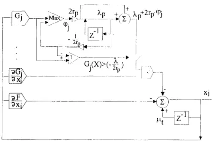
FIG. 4. Circuit of a constrained nonlinear optimization solver based on the ALM method.

The parallel structure corresponding to equation (24) is proposed and shown in Fig. 4, where the step size I~t is adopted as a constant. The main feature of this architecture is that it uses the ALM method, which converges more quickly than other penalty methods. This optimization circuit is not like the neural networks described in Section 2, but it has many of the features of neural networks. For example, this circuit performs massive parallel processing of analog signals and is capable of adapting the connection weights to accelerate convergence during the optimization process.

3.3. Procedure for N N B A C O system in end milling

The proposed N N B A C O system is shown in Fig. 5, in which there are two different kinds of neural networks employed. Neural network (I) is used to learn the appropriate mappings between the input and output variables of the machining process, so we shall refer to it as the neural network for modeling. This neural network is a three-layered back-propagation network with three input nodes, each representing feedrate per tooth, axial depth of cut, and radial depth of cut, and four output nodes, i.e. the forces in the X and Y directions, cutting power, and the surface finish of the workpiece.

Neural network (II), which is described in Section 3.2, is used to determine the optimal inputs, so we shall refer to this network as the neural network for optimization. Since neural network (I) is used to describe the cutting process, the derivatives in equation (24) can be calculated by a forward pass through the back-propagation network. The detailed derivation is shown in the Appendix. This can greatly reduce computing time in solving the optimization problem.

The procedure of this N N B A C O system can be summarized as follows:

7

. ~ Neural network I

for modeling

Current ~l state

. ~ Neural network 11 I

for optimization .Optimal inputs

Measured outputs

(9)

STEP 1 Under the initial constraints, neural network (II) determines a set of optimal inputs and then sends them into the milling machines and neural network (I). STEP 2 The measured outputs of the milling machine, corresponding to the optimal

input, are used as the desired output to train neural network (I).

STEP 3 Neural network (II) uses the newly upgraded neural network (I) as the model of the end milling process to find the optimal inputs and sends them into the milling machine and neural network (I).

STEP 4 STEP 2 and STEP 3 are repeated until the termination of the cutting process.

4. SIMULATION

In the following, the theoretical model of the end milling process is described. A simulation employing this theoretical model and the results are presented to confirm the feasibility of the NNBACO system.

4.1. Theoretical m o d e l s o f e n d m i l l i n g

Since there are four cutting constraints taken into account in this simulation (the average cutting force in the X, Y directions, cutting power and surface finish) we use four corresponding theoretical models to describe the end milling. These models are presented below.

The theoretical models for the average cutting forces in the X, Y directions presented

by Lee et al. [17] are expressed as

Fx = K t ' N t ' f t ' A a ' { K r ' [ s i n ( 2 " f 3 e n ) - 2"[3e,] + [1 -- COS(2"13en)]}/(8"rr) (N)

Fv = K , . N t . f t . A d ' { K r ' [ 1 - cos(2.13c,)] + [2"13~n -- sin(2.13~,,)]}/(8.'rr) (N), (26) where 13¢n is the tooth entry angle, Nf is the tooth number of the end mill, Kt indicates the ratio of tangential cutting force to the chip load, and Kr indicates the ratio of radial to tangential cutting force. Kt and Kr for the aluminum with hardness 55 HRB are

Kt = 757.7045 • f t ° ° 5 5 s (N/mm 2)

Kr = 0.2627. f-(, 2279 . (27)

The theoretical model for the cutting power can be expressed as

P = 1.6 + 4.26- [(N,. A,~ • Rd • ft) 0"66] " rpm/97422 (kW), (28)

where rpm is the spindle speed, expressed in revolutions per minute. According to [18], the surface finish of the workpiece can be modeled by

Ra = ~ / ( 8 . R) (mm) (29)

in which R a is the average peak to valley height on the workpiece surface and R is

the radius of the end mill. The deformation of the cutting tool is ignored here.

4.2. C o m p u t e r s i m u l a t i o n a n d results

In order to investigate the stability and adaptation of the NNBACO system, we simulated a procedure similar to that described in Section 3.3 and the real end milling process was replaced by the theoretical model, i.e. equations (26)-(29).

Since an untrained neural network has no knowledge about the system, unpredictable results may be obtained. Therefore, initial training was applied to neural network (I). In initial training, the first step is to generate the I/O samples from the theoretical model. Different values spanning the allowable range of each input variable yield a total of 420 input combinations. These input variables were used to determine the

(10)

output quantities, and they composed the set of I/O samples which were used for initial training and testing.

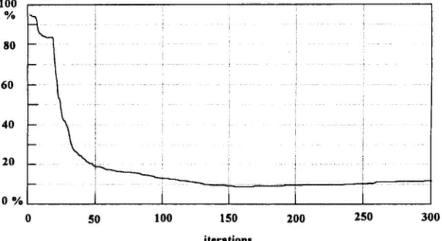
The three-layered back-propagation network with three inputs and four outputs described in Section 3.1 was employed for neural network (I). In the initial training, we start with three hidden nodes and the number of nodes was increased until a low error rate was achieved. The error rate is the ratio of incorrect samples, i.e. samples in which the absolute difference between the theoretical output and the output of the neural network exceeds 10%, to all 420 samples. The simulation results for the initial training, with ten hidden-layer nodes, are shown in Fig. 6; the results indicate that after 150 iterations the error rate approached 10%.

If the number of iterations used in training the neural network is increased, the error rate may be reduced slightly. But, from a macroscopic point of view, the error rate remains in the vicinity of 10%. Increasing the number of nodes in the hidden layer may also decrease the error rate, but it may make it more difficult to realize the proposed structure physically and may cause more time to be consumed in calculating the optimal inputs. Hence ten hidden-layer nodes were chosen in this stage.

According to the experiment set-up and workpiece used in our laboratory, the limits on the input and output variables that were used in the simulation were as follows: The upper limitation on the input variables:

ft: 0.33 (mm/tooth) Ra: 12.5 (mm) Ad: 24.5 (mm) . The allowable outputs:

Fx:800(N) ~ : 1 6 0 0 ( N )

e:l.8(kW)

Ra:0.0015(mm).

In order to examine the performance of the NNBACO system under specific cutting conditions, one of the input variables (radial depth of cut) was specified as varying between three specific values, and it changed from one value to another every one hundred iterations. Through this simulation, not only the static (constant Ro) but also the dynamic (varying Rd) performance of this system were investigated.

I 0 0 % 80 60 4O I ~ _i" i 20 . . . i i 0 % I . 0 50 100 150 200 250 300 i t e r a t i o n s

(11)

Adaptive Control Optimization 647

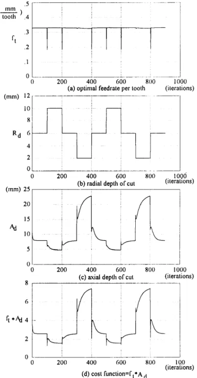
Figure 7(b) shows the three values (2, 6 and 10 mm) for the radial depth of cut,

and Figs 7(a) and (c) show the corresponding optimal inputs

(Aa

and ft). Because the

neural network can not "learn" as fast as the change in the radial depth of cut, there were some transient states at the beginning of each state. When the radial depth of cut is 2 mm, the inequality constraints of the cutting power are satisfied more easily than when the depth is 6 or 10. Hence the product of Jet and Rd, shown in Fig. 7(d), has the greates t value when

Ra

= 2. In these figures, we also find that as the system varies, the steady optimal inputs do as well.

The neural network's outputs corresponding to the optimal inputs are shown in

.5 I l l m

( ~ ) , 4

,3

ft .2 .1 0 0 ( m m ) 12 10 8 R d 6 4 2 0 0 ( m m ) 25 20 15 10 ; i 200 400 600 800 1000

(a) optimal fee&ate per tooth (iterations)

V

200 400 600 800 .. 1006 .

(b) radial depth of cut 0teratlons)

i

f

0 200 400 600 800 1000

(c) axial depth of cut (iterations) 8 ft*Ad 4 2 0 0 200 400 600 800 100 (iterations) (d) cost function--ft*A d

(12)

648 SHIUH-TARNG CHIANG et al.

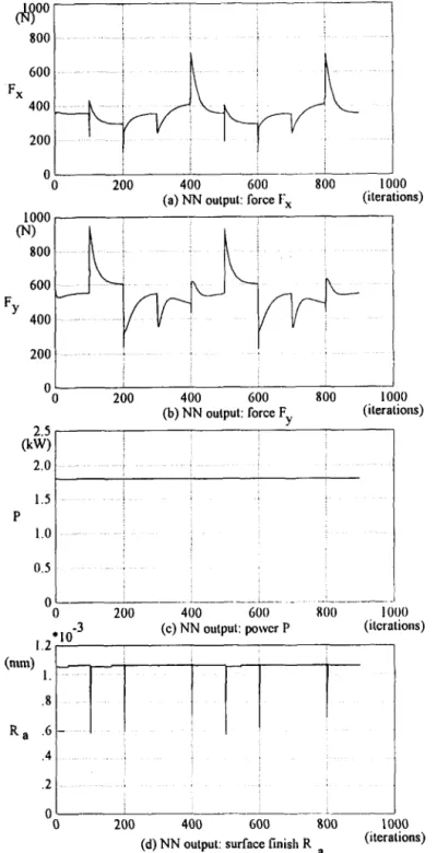
Fig. 8. Because the calculation of the optimizer is based on the neural network, all the inequality constraints, i.e. equation (23), are satisfied. However, in order to satisfy the inequality constraints for the cutting power, all the other outputs of the neural networks are far from the upper limits.

Most of the outputs of the theoretical model, shown in Fig. 9, are below the maximum

limitations. But some overshoots can be detected in the cutting power during the

changes between states. We also find that in these figures the maximum MRR is mainly limited by the cutting power.

The learning errors in the simulation are shown in Fig. 10, in which the error is defined as follows (-#cc- : ;-; -: 800 , I 600 Fx 400 200 0 0 200 400 600 800 IO’ ₄₀

(a) NN oulpul: force Fx (ileratlons)

1000 09 800 600 FY 400 200 2;o 400 600 800 1000

(b) NN output: force F,, (ileralions)

I

400 600 800 IO00

(c) NN output: power P (ilcralions)

_-_- -~

200 400 600 800 1000

(d) NN output: surface finish R _a (iteralions) FIG. 8. Neural network outputs in simulation.

(13)

600 i . . . i ...

Fx 400 ~ ...

201 ...

0 200 400 600 800 1000

(a) milling output: force F x (iterations)

10001 ~ soo ... i ... ... i . . . . 600 . . . Fy 400 ~ ... ~ ... ... 7 ~ ... : . 200 ... ] ... i ... ol i i 0 2 . 5 (kW) (ram) 2.0 1.5 1.0 0.5 200 400 600 800 1000

(b) milling output: force F y (iterations)

r - - - i v - ~ : 0 1.2"10 -3 I. .8 R a .6 .4 200 400 600 800 1000

(c) milling output: power P (iterations)

.2 . . . T

0 i

0 200 400 600 800 1000

(d) milling output: surface finish R _a (iterations)

FIG. 9. Outputs from the theoretical model in simulation. Itheoretical o u t p u t - n e u r a l n e t w o r k o u t p u t I

e r r o r = t h e o r e t i c a l o u t p u t (30)

B e c a u s e o f large v a r i a t i o n o f w e i g h t s at the b e g i n n i n g o f s t e p c h a n g e in Rd, the o p t i m i z e r t a k e s m o r e i t e r a t i o n s to find a set o f o p t i m a l inputs. A s the n e u r a l n e t w o r k a p p r o a c h e s the s t e a d y state, the o p t i m a l inputs can b e o b t a i n e d in f e w e r iterations. This m e a n s t h a t t h e n e u r a l n e t w o r k can d e s c r i b e the s y s t e m m o r e a n d m o r e a c c u r a t e l y in the static state. C o m p a r e d with t h e results o f initial training, the e r r o r d i m i n i s h e d v e r y quickly.

(14)

650 SHIUH-TARNG CHIANG et al. R a (x 100%) 10 0.8 0.6 0.4 0 2 0 i , , i i (x 100%) 1.0 I 0.8 0.6 /

ikL

200

_LI

400 600 (a) F x error 800 1000 (iterations) Fy 0 200 400 600 800 1000 (x 100%) (b) Fy error (iterations) 0.1 0.08 o.o .... ! P 0.04 ] i 0.02 0 0 (x 100% 1.0 0.8 0.6 0.4 0.2 0 200 400 600 800 1000

(c) power error (iterations)

2OO 400 600 800

(d) surface finish error

1000 (iterations) FIG. 10. The learning errors in the simulation.

After the simulations in this section, we adopted some patterns from the initial training set to test the underlying neural network and found that for patterns located near the optimal inputs the neural network generated outputs with a very small error. But for patterns far from the optimal values, the network generated outputs with a large error. This result implies that the neural network has only partial knowledge after training.

(15)

Adaptive Control Optimization

651 5. EXPERIMENTS

5.1. Experimental set-up

We conducted a series of experiments with end milling to confirm the feasibility of the proposed N N B A C O system.

The experimental set-up for the N N B A C O system is shown in Fig. 11, which also defines the positive directions of the three axes. The feedrate command to the servo- driver was generated by a hardware interpolator. Each NC servo loop (per axis) included a DC servo motor and a P.I.D. Velocity and position feedback were provided by tachometer and encoders.

A vertical knee-type milling machine (3 horse power spindle motor) was used for the experiments. The cutting forces were measured by a dynamometer (Kistler 9257B) and a charge amplifier (Kistler 5007). The A / D converter used was a 12-bit one; the collected data were saved to the memory of a 486 personal computer by D M A (direct memory access) transfer. The sampling time in the A / D converter was 1 ms and the NNBACO system updated the feedrate parameter in 100 ms.

The data processing and the control algorithm were implemented using Borland C+ + V.3.0 on a 32-bit 486 PC. The other machining conditions and parameters of the workpiece are listed below:

Workpiece: aluminum alloy (T6061). Cutting tool: end mill,

25 mm diameter, four teeth,

160 mm total length. Cutting conditions:

spindle speed: 300 rpm, axial depth of cut: 25 mm. No coolant.

5.2.

Experiments

We conducted three main series of experiments, in which two differently shaped workpieces were machined. Details of the experimental conditions and the dimensions of the workpiece are shown in Figs 12(a) and (b).

The first experiment is conventional cutting that the feedrate per tooth was set to be constant under the constraints on the maximum allowable cutting forces.

In the second experiment, the proposed N N B A C O system was applied in the end milling to demonstrate its performance. Because of the limitations of the laboratory equipment used, the neural network for modeling was set up with only two outputs, Fx and

Fy,

and the axial depth of cut was kept at 25 mm. There were ten nodes in the hidden layer. The radial depth of cut and other cutting conditions were set up as described in Figs 12(a) and (b).

In the last experiment on each workpiece, regardless of the variation in radial depth

feed direction

[ ~

~~1

workpiece

dynamometer

I

~.~

hardware table

I l

[ 486 pc I I interp°lat°r

~ NC servo

X-axis

T

X Charge /

Y amplifier

i

FIG. 1 1. The experimental set-up.

(16)

652 SHIUH-TARNG CHIANG et al. (a) Down milling Workpiece A:

4 I-

90 40 --~ 1 3 (unit: iron) Experiment 1 (Constant feedrate) Experiment 2

(NNBACO system is apply)

Experiment 3

(Rd to NN is kept constant -7 2 ram)

Maximum allowable force

Case: case a-I

Cutting condition ft: 0.12 ram/tooth Result: Figure 13

Case: case a-2

Cutting condition ft: 0.075-0.25 Iron/tooth Result: Fisure 14

Case: case a-3

Cutting condition ft: 0.075-0.25 iron/tooth Result: Figure 15 Fx: 400 N, Fy: 450 N (b) Down milling Workpiece B: 90 -4-25--,.- 1 ~r 2 i

T

(unit: ram)

Experiment 1 Case: case b-I

(Constant feedrate) Cutting condition ft: 0.12 nun/tooth

Result: Figure 16

Experiment 2 Case: case b-2

(NNBACO system is apply) Culting condition It: 0.075-0.25 nun/tooth

Result: Figure 17

Experiment 3 Case: case b-3

(Rd to NN is kept constant Cutting condition It: 0.075-0.25 iron/tooth

= 2 1ran) Result: Figure 18

Maximum allowable force - - Fx: 400 N, Fy: 450 N

Fro. 12. (a) Cutting conditions for workpiece A. (b) Cutting conditions for workpiece B.

of cut, the input (radial depth of cut) to the neural network was fixed at specific "false" values as defined in Figs 12(a) and (b). The difference between the "real" and "false" input is like a noise value. Thus, the error tolerance of the N N B A C O system can be investigated from this experiment.

(17)

5.3. Results and discussion

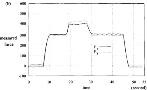
The geometry of the first workpiece, shown in Fig. 12(a), consisted of two steps. In order to satisfy the force limitation (the maximum allowable forces in the X, Y directions were 400 and 450 N, respectively), the feedrate was kept at 0.12 (mm/tooth) in case a-1. The measured force is shown in Fig. 13.

The N N B A C O system was applied in case a-2, in which the feedrate decreased to a lower level as the cutting tool stepped up to a higher stair. The results are shown in Fig. 14. The error defined is similar to equation (30), but the theoretical outputs are replaced by the measured signals. Since the neural network cannot learn very accurately when the radial depth of cut changes, there are two peaks in the measured force. After a while, however, the measured force in the X direction stabilized around the preset value, which means that the optimal cutting conditions are constrained by the force in the X direction in this case. Due to the sudden change in the input to the neural network, there is a peak in the neural network's output shown in Fig. 14(c).

Although the radial depth of cut varied from 2 to 3 mm, the input to the neural network was kept at 2 mm throughout the tool path in case a-3. The results, as depicted in Fig. 15, show that the peak in the neural network's output vanished, because there was no change in the input to the network. However, the two peaks are still present in the measured force and the error diagram, i.e. Figs 15(b) and (d).

For the other cases of experiment, there were three steps in the second workpiece, and the distance between each step was shorter. This workpiece, as shown in Fig. 12(b), includes ascending and descending parts. The maximum allowable forces in the X, Y directions were again set as 400 and 450 N, respectively.

In case b-l, feedrate was kept at 0.12 (mm/tooth). The measured forces are shown in Fig. 16.

The results of case b-2 obtained using the N N B A C O system are shown in Fig. 17. For the same reasons described in case a-2, there are four peaks in the neural network's output. In Fig. 17(c), we see that the optimal cutting conditions are limited sometimes by the force in the X direction and sometimes by the force in the Y direction. From the Fig. 17(d), we see that the error in the third step is not less than that in the first step. It means that the system only possesses knowledge near about optimun region. As the state (Rd) returns to the previous state, the system also needs to reoptimize the cutting conditions as before.

(N) m e a s u r e d force 600 500 400 300 200 100 0 -!00

m

i F x i F y ... 10 20 30 time FIG. 13. The results of case a-].

40 50 55

(second)

(18)

654

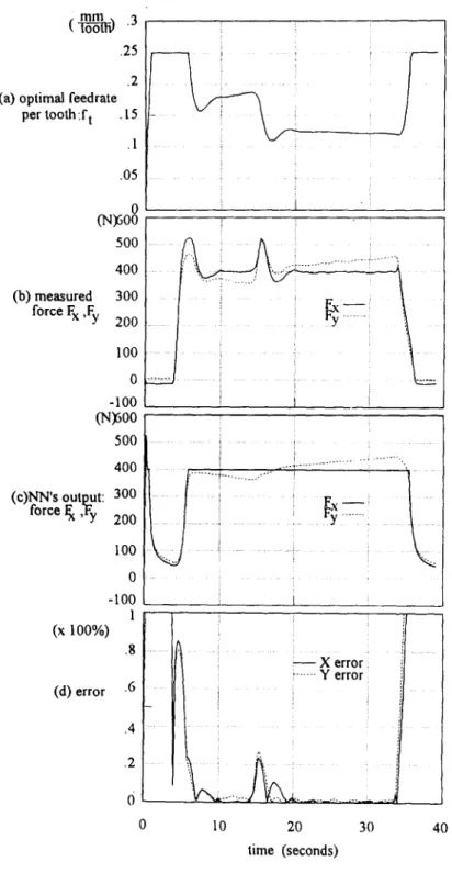
( -to-I~[~ .J

.25 .2 (a) optimal .fee&ale

per tootla:f t .15 .I .05 0 (W)600 500 400 (b) measured 300 forces Fx,Fy 200 100 0 -100 (N~600 500 400 (c)NN's output: 300 forces Fx,Fy 200 100 0 -100 l (x ! 0 0 % ) .8 (d) error .6

SHIUH-TARNG CHIANG el al. .3 , i ~ i ! ... i . . . i . . . L . . . i.--:-/.i.Z ... .4 .2 ~ - - x error!

il

i ... v error i

0 10 20 30 time (seconds) Fro. 14. The results of case a-2.

40

For the results of the last case b-3, Fig. 18, as in the previous case, we see that the optimal conditions are always constrained by the maximum allowable force in the X direction. When the results of Figs 17(d) and 18(d) are compared, they seem to be different. In the case of Fig. 17(d), as the radial depth of cut changes, the input of neural network suddenly changes which causes the weights to update tremendously and generates larger force errors. In the case of Fig. 18(d), this situation is avoided

(19)

Adaptive Control Optimization 655 .25

.2 (a) optimal feedrate

per tooth:f t .15 .1 .05 0 ~)600 500 400 (b) measured 300 force F x ,Fy 200 100 0 -100 ~)600 500 400 (e)NN's output: 300 force F x ,Fy 200 100 (x 100%) (d) error ¸ , i i ¸ ... ... i 0 . . . . i • -100 i X error i ... Y error 10 20 30 time (seconds) I ... 40 1 .8 .6 .4 .2

FIG. 15. The results of case a-3.

and s m o o t h transitions o f the e r r o r s o c c u r as true radial d e p t h of cut changes. H o w e v e r , for large v a r i a t i o n o f d e p t h o f cut, the N N B A C O still n e e d to give c o r r e c t input to r e d u c e the c o n v e r g e n c e time.

T h e results o f the real-time c o n t r o l e x p e r i m e n t s p r e s e n t e d a b o v e s h o w that w h e n applied in e n d milling the N N B A C O s y s t e m is stable within the range o f the cutting conditions e x a m i n e d . Since the cost f u n c t i o n is M R R a n d the radial a n d axial d e p t h

(20)

656 SHIuH-TARNG CrUANG et al. (N) measured force 600 500 400 300 200 100 0 -100 Z L'-i/-"i/ " "i.

i i

,

Fx-

ti -

. . . . 0 10 20 30 40 time 50 55 (second)

FIG. 16. The results of case b-1.

of cut are kept at specific values in each case studied, we can use the time needed to cut through the workpiece as an index of efficiency. That is, the less time spent, the higher M R R is. The time spent in cutting through each workpiece is given in Table 1. From the table, it is clear that when the N N B A C O system is applied M R R is increased greatly.

Although a "false" input was applied in the last experiment on each workpiece, the M R R for these experiments is still high. Moreover, in some cases, because of less variation in the neural network's input (Ra), these cases perform better than the "true" input cases. This shows that the N N B A C O system is an architecture with high fault tolerance.

6. CONCLUSIONS

In this paper, an architecture is presented for on-line determining optimal cutting conditions in an end milling process. The proposed N N B A C O system, which includes two different neural networks, differs from conventional adaptive control with optimization (ACO) systems in that (1) multi-constraints are handled simultaneously without increasing the processing time; (2) no specific model exists, but rather a back-propagation network is employed and (3) a special optimal mechanism is adopted to determine optimal cutting conditions.

Although the two neural networks in the N N B A C O system are not realized by chip technology, the simulations and experiments presented here show that this architecture can effectively describe the behavior of end milling and increase the cutting efficiency. Because the neural network (II) performs the optimization in the NNBACO system, neural network (I), the modeling network, only possesses knowledge in the vicinity of a local optimum. In the simulations and the experiments described here, although

T A B L E 1. T I M E SPE NT IN E N D MILLING WITH RESPECT TO DI FFER ENT WORKPIECE SHAPES

Workpiece A Workpiece B

Experiment 1 Case case a-1 case b-1

(Feedrate keeps constant) Time 54.2 s 54.2 s

(Apply NNBACO) Time 40.0 s 34.9 s

(21)

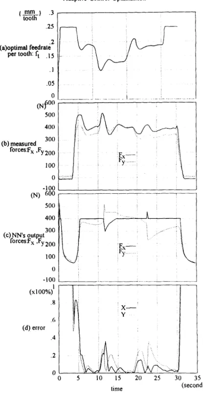
Adaptive Control Optimization 657 I mm ) .3 i-6-6ih- .25 .2 (a)optimal feedrate per tooth: ft .15 .1 .05 0 (NJ 500 500 400 300 (b) measured forces:F x ,Fy 200 100 0 -100 (N) 600 500 400 300 (c) NN's output forces:F x ,Fy 200 100 0 -100 I (x100%) .8 .6 (d) error .4 i I

L

0 - . \ . . . . - _ . . . - ° - - , Fx F~,. ', .2 X Y 10 15 20 25 30 35 lime (second)

FIG. 17. The results of case b-2,

there were some errors in the beginning, the N N B A C O system gradually achieved optimal cutting conditions. A n d since the N N B A C O system itself determines the knowledge to be acquired, i.e. by the neural network for optimization, it behaves like a self-organizing system.

The N N B A C O system is applied to end milling in this paper, but it is obvious that this system is a general-purpose architecture, i.e. it can be extended to other machines to improve cutting efficiency.

(22)

658 SHIUH-TARNG CHIANG et al. (_lnnL.~ .3

tooth j .25

.2 (a) optimal feedrate

tooth: per fl .15 .1 .05 0 (N) 600 500 4OO 300 (b) measured forces: Fx ,Fy200 100 0 - I 0 0 (N) 60O 500 400 300 (c) NN's output forces: F x ,Fy200 100 0 -100 1

(x 100%)

.8 ,6 (d) error .4 .2

/ - - /

Fx- i t"- " " .... "" " ... ""

i/

! 0 5 10 15 21) 25 time 30 I

J

I 35 (second) FIG. 18. The results of case b-3.

REFERENCES

[ 1 ] Y. KOREN, Computer Control of Manufacturing System. McGraw-Hill, New York (1983). [2] M. A. ELBESTAWl, A S M E J. Dyn. Syst. Meas. Control 112, 6ll (1990).

[3] G. CHRVSSOLOUmS and M. GUmLOT, A S M E J. Engng Ind. 112, 122 (1990). [4] G. R. MADEY, J. WEINROTH and V. SHAH, J. lntell. Manufact. 3, 193 (1992).

[5] S. R. RANGWALA and D. A. DOaNFELD, I E E E Trans. Syst. Man Cyber. 19, 299 (1989).

[6] G. S. CHOI, Z. WANG and D. A. DORNFELD, Proc. IEEE, Int. Conf. Robotics and Automation 1567 (1991).

[7] J. CHEN, M. A. SHANBLA'rr and C. MAA, Int. J. Neural Syst. 2, 331 (1992). [8] D. W. TANK and J. J. HOPFIELD, 1EEE Trans. Circuits Syst. CAS-33, 533 (1986). [9] L. O. CHUg and G. N. LIN, I E E E Trans. Circuits Syst. CAS-31. 182 (1984).

(23)

Adaptive Control Optimization 659 [11] A. RODRIGUEZ-VAZQUEZ, R. DOMINGUE7, A. RUEDA, J. L. H.r;ERTAS and E, SANCHEZ, I E E E Traits.

Circuits Syst. 37, 384 (1990).

[12] A. CiCHOCrd and R. UNBEHANEN, Int. J. Orcuit Theory Appl. 19, 161 (1991).

[ 13] D. RUMELnART and J. L. McCLELLAND, Parallel Distributed Processing: Explorations in the Microstruc- ture of Recognition, Vols 1 and 2. MIT Press, Cambridge, MA (1986).

[14} K. S. NARENDRA and K. PARTHASARATHY, IEEE Trans. Neural Networks 1(4), (1990).

[15] G. N. VANDI':aPLAATS, Numerical Optimization Techniques for Engineering Design: with Application. McGraw-Hill, New York (1984).

[16] R. T. ROCKAFELLER, J. Opt. Theory Appl. 12, 555 (1973).

[17] A. C. LEE, S. T. CH]Ar,~G and C. S. LIu, J. Chinese Soc. mech. Engrs 12, 412 (1991). [18] M. C. SHAW, Metal Cutting Principles. Oxford University Press, New York, (1984).

APPENDIX

In this Appendix, the method used to calculate the derivatives of equation (24) by a forward pass through the network is described. With regard to Fig. 2, we define the following nomenclature:

net~.k the sum of the ith neuron's inputs in the kth layer, i.e.

Oi.k

net/., = ~ [wi.j.k ' o,,k-I] (A1)

]

the ith neuron's output in the kth layer, i.e. o,.k = f(neti.k)

if f(.) is a sigmoid function then equation (A2) becomes

(A2) 1 f(net,.k) = (A3) 1 + e--nct~.k Yi di Wid,k E

the output of the ith neuron in the output layer. If the neural network has three layers then Yi = 0t.3"

the desired output of the ith output node.

the weight between the ith neuron in the kth layer and the jth neuron in the (k - 1 ) t h layer. defined as the global error

E = 0.5 • ~ ( d , - O,.k) 2 . ( A 4 )

i