Determination of optimal converting point of
color temperature conversion complied with
ANSI C78. 377 for indoor solid-state lighting and
display applications
Yao-Fang Hsieh,1 Mang Ou-Yang,2,* Ting-Wei Huang,2 and Cheng-Chung Lee1 1Department of Optics and Photonics, National Central University, 300 Jhongda Rd., Jhongli City, Taoyuan County,
320 Taiwan
2Department of Electrical and Computer Engineering, National Chiao-Tung University, 1001 Ta-Hsueh Rd., Hsinchu City, 30010 Taiwan
*oym@cc.nctu.edu.tw
Abstract: In recent years, displays and lighting require color temperature
(CT) conversion function because observers have different preferences. This paper proposes effective methods to determine the optimal converting point of CT conversion for display and lighting application. For display application, the concepts of center of gravity and isotemperature line are applied to determine the optimal converting point. The maximal enhancement of luminance between the optimal and average is 18%. For lighting application, this paper proposes two methods to determine the optimal converting point in the CT quadrangle which complies with ANSI C78. 377. The enhancement of luminance in two CT modes (5700K and 6500K) are 14.2% and 23.6%, respectively.
©2012 Optical Society of America
OCIS codes: (120.2040) Display; (150.2950) Illumination; (230.3670) Light-emitting diodes;
(330.1690) Color; (330.1710) Color, measurement. References and links
1. A. Borbély, A. Sámson, and J. Schanda, “The concept of correlated colour temperature revisited,” Color Res. Appl. 26(6), 450–457 (2001).
2. K. L. Kelley, “Lines of constant correlated color temperature based on MacAdam’s (u,v) uniform chromaticity transformation of the CIE diagram,” J. Opt. Soc. Am. 53(8), 999–1002 (1963).
3. A. R. Robertson, “Computation of correlated color temperature and distribution temperature,” J. Opt. Soc. Am.
58(11), 1528–1535 (1968).
4. D. B. Judd, “Estimation of chromaticity differences and nearest color temperature on the standard 1931 ICI colorimetric coordinate system,” J. Opt. Soc. Am. 26(11), 421–424 (1936).
5. J. Schanda and M. Danyi, “Correlated color-temperature calculations in the CIE 1976 chromaticity diagram,” Color Res. Appl. 2(4), 161–163 (1977).
6. M. Krystek, “An algorithm to calculate correlated colour temperature,” Color Res. Appl. 10(1), 38–40 (1985). 7. Q. Xingzhong, “Formulas for computing correlated color temperature,” Color Res. Appl. 12(5), 285–287 (1987). 8. C. S. McCamy, “Correlated color temperature as an explicit function of chromaticity coordinates,” Color Res.
Appl. 17(2), 142–144 (1992).
9. M. Ou-Yang and S. W. Huang, “Determination of gamut boundary description for multi-primary color displays,” Opt. Express 15(20), 13388–13403 (2007).
10. S. Wen, “Design of relative primary luminances for four-primary displays,” Displays 26(4–5), 171–176 (2005). 11. L. Honam, C. Hyungjin, L. Bonggeun, P. Sewoong, and K. Bongsoon, “One-dimensional conversion of color
temperature in perceived illumination,” IEEE Trans. Consum. Electron. 47(3), 340–346 (2001).
12. D. S. Park, S. K. Kim, C. Y. Kim, W. H. Choi, S. D. Lee, and Y. S. Seo, “User-preferred color temperature conversion for video on TV or PC,” Proc. SPIE 5008, 285–293 (2003).
13. S. K. Kim, D. S. Park, W. H. Choi, and S. D. Lee, “Color temperature conversion for video on TV or PC reflecting human's display preference tendency,” in Proceedings of IEEE Conference on Convergence Information Technology (Institute of Electrical and Electronics Engineers, Gyeongju, 2007), pp. 861–867. 14. ANSI_NEMA_ANSLG C78.377–2008.
15. M. Ou-Yang and S. W. Huang, “Design considerations between color gamut and brightness for multi-primary color displays,” J. Display Technol. 3(1), 71–82 (2007).
1. Introduction
In lighting, color displays, photography and other fields, color temperature (CT) represents the chromaticity of visible light. The CT of a light source corresponds to the same chromaticity of the Planckian radiator at that temperature. The chromaticity diagram of the Commission International de l’Eclairage (CIE) shows the Planckian chromaticity coordinates locus of various CT. People can calculate the Planckian locus by colorimetrically integrating the Planck function at many different CT, with each temperature specifying a unique pair of CIE 1931 xy chromaticity coordinates on the locus. However, the chromaticity of several natural and artificial light sources is not on the Planckian locus. Thus, the concept of correlated color temperature (CCT) is used. The CCT has been defined as “the temperature of the Planckian radiator whose perceived color most closely resembles that of a given stimulus seen at the same brightness and under specified viewing conditions” [1]. The CCT is commonly used to designate the color of light which includes skylight, daylight, fluorescent light, and other illuminations. Kelly [2] proposed a graphical method for finding CCT on a diagram. Robertson [3] proposed methods to evaluate numerically CCT from the distribution of the spectral power. Judd [4] proposed the concept of isotemperature lines for the calculation of CCT for the selected radiator. The CCT of the light source can be determined by extending the isotemperature line from the Planckian locus out to the chromaticity coordinate of the light source. If the chromaticities were plotted in uniform color space, isotemperature lines were straight lines perpendicularly intersecting with Planckian locus. Six isotemperature lines were plotted on the CIE 1976 u’v’ chromaticity diagram [5]. The computation of CCT and determination of the isotemperature line have also been studied in other previous researches [6,7]. The method of Qiu was better than Krystek, but it involved different equations in two ranges of an angle. The method was more complicated than the McCamy [8] which proposed a simple equation to compute CCT from CIE 1931 xy chromaticity diagram.
The CT conversion is an important issue for display and LED lighting. For display application, consumers have different preferences to the CT. According to the color mixing theory and the relationship between color gamut area and luminance [9], when the reference white point is converted to the point of target CT, the luminance must be sacrificed. In the same color perception condition, less luminance loss means less power consumption for lighting and display. Therefore, Wen [10] proposed a theory using linear approach to obtaining maximal luminance of the point of target CT. However, the process of calculation was complicated. In addition, he did not propose any method to determine the optimal converting point of target CT. Some recent investigations suggested methods to implement CT conversion [11–13]. These researches established the user-preferred CT model from the experiment and determined the optimal converting point of CT conversion from their model. However, they did not consider determining the optimal converting point on the isotemperature line and the issue about luminance loss. The CT conversion is also a very important issue for LED lighting. The LED needs different CT illumination for different applications. The ANSI (American National Standard Institute) proposes a standard document (ANSI C78.377) to gauge eight BINs which include warm (2700K, 3000K, 3500K), normal (4000K, 4500K), and cold (5000K, 5700K, 6000K) modes, for Solid State Lighting (SSL) products [14]. These eight BINs are approved by the ENERGY STAR. This standard specifies the range of chromaticities recommended for general lighting with indoor SSL products, and guarantees the white light chromaticities of products can be communicated to consumers. The chromaticity of light is represented by chromaticity coordinates (x,y and
u’,v’). The standard defines the range of CCT as a quadrangle (7-steps from Planckain locus). The chromaticity tolerance is based on MacAdam ellipses to define the perceptible color difference. The appendix of the standard includes table for the chromaticity coordinates of the center points and the four corners of each quadrangle. Because the CIE 1976 u’v’ chromaticity diagram is more uniform than the CIE 1931 xy chromaticity diagram and the
CCT is defined on the CIE 1960 (u’,2/3v’) chromacitity diagram, this paper derives the proposed algorithms based on the CIE 1976 u’v’ chromaticity diagram.
This paper mainly proposes methods for determining the optimal converting point of target CT for CT conversion. In applications, the display and SSL have different definition of the range of CCT. The range of CCT of display is the isotemperature line and of the SSL is the CT quadrangle. This paper individually describes the methods for these two applications. In our previous research [15], the algorithm for effectively obtaining the maximal luminance of the point of target CT has been proposed. This paper applies the previous algorithm to obtain the maximal luminance of the optimal converting point. Finally, simulations and experiments are performed to verify the methods.
2. Theory
2.1 The method for determining the optimal converting point of CT conversion for display application
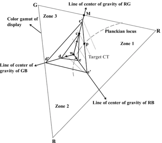
The proposed method converts the reference white point to the color point on the isotemperature line of the target CT. There are many color points on the isotemperature line. Which point on the isotemperature line is the optimal converting point? This paper defines that the optimal converting point has the maximal luminance among the color points on the isotemperature line and the worst point has the minimal luminance. According to the color mixing theory and the relationship between color gamut area and luminance [9], when the color gamut area expanded to bigger one, the luminance must be decreased. Hence, the proposed method determines the optimal converting point on the isotemperature line first meeting by the expanded color gamut from the reference white point. Huang [9] also proved that the color gamut area must expand along the lines of center of gravity of tri-primaries. The concept of line of center of gravity was from the Centre of Gravity Law of Color Mixture [16]. When two colors C1 and C2 were additively mixed, the resulting color C3 was located on the line jointing C1 and C2 in a position given by the Centre of Gravity Law of Color Mixture. The line jointing C3 and reference white point was called line of center of gravity of C1C2. Figure 1 is used to explain the proposed method. The dotted lines represent the isotemperature line. The dashed line represents the Planckian locus. The point p on the Planckian locus is chosen to be the target CT for example. When the luminance of R, G, and B are full input, the color gamut area is shrunk to a single point (point W; reference white point). As the luminance decreases, the single point is expanded to the triangle cde along the lines of center of gravity (RG, GB, and RB). When the luminance decreases again, these three apexes (the points c, d, and e) of the triangle also move along the lines of the center of gravity (RG, GB, and RB) and the area of the triangle increases (the triangle changes from cde to c’d’e’). Hence, when the reference white point is converted to the isotemperature line of target CT, the c is the optimal converting point. Because the point c is first met by the expanded color gamut from reference white point, the area of triangle cde is smaller than other triangles which are constructed by point on isotemperature line and the points on the lines of center of gravity RB, GB (for example, the area of triangle c’d’e’ is bigger than triangle cde). Therefore, the optimal converting point is the intersection between the line of center of gravity and the isotemperatue line. In addition, the lower CT is on the right side of the reference white point (W). Hence, when the target CT is lower than the reference white point of display, the optimal converting point of target CT can be obtained from the intersection between the line of the center of gravity RG and the isotemperature line. When the target CT is higher than the reference white point of the display, the optimal converting point can be obtained from the intersection between the line of the center of gravity GB and the isotemperature line.
Fig. 1. The schematic of the determination of optimal converting point of target CT. The point c is the optimal converting point which is also the intersection between the isotemperature line of target CT and line of center of gravity RG.
2.1.1 The chromaticity coordinate of the optimal converting point of CT conversion
According to the description of previous section, the optimal converting point of target CT is the intersection between line of center of gravity and isotemperature line. This section introduces the equations of these two lines. The equation for the line of the center of gravity, Eq. (1), is derived using color mixing theory and the concept of slope. The line of the center of gravity of RG is considered in an explanatory example. Figure 1 shows, the line of the center of gravity of RG is constituted by point B and point M. The chromaticity coordinate and luminance of M can be determined by the color mixing of R and G. Then, points B and M are utilized to obtain the equation for the line of the center of gravity of RG.
( ' ' ) ( ' ' ) ( ' ' ' ' ) ( ' ' ' ' ) ' ' , ( ' ' ) ( ' ' ) ( ' ' ) ( ' ' ) i i k j j k i i k k i j j k k j i i k j j k i i k j j k m v v m v v m u v u v m u v u v v u m u u m u u m u u m u u − + − ⋅ − ⋅ + ⋅ − ⋅ = + − + − − + − (1)
where (u’i, v’i), (u’j, v’j), and (u’k, v’k) are respectively the chromaticity coordinate of the
primary color i, j and k. Moreover, mi = Yi,MAX/v’i, mj = Yj,MAX/v’j, mk = Yk,MAX/v’k. When i, j, and k represent R, G, and B, respectively, Eq. (1) is the equation for the line of the center of gravity of RG. When i, j, and k represent G, B, and R, respectively, Eq. (1) is the equation for the line of the center of gravity of GB. When i, j, and k represent B, R, and G, respectively, Eq. (1) is the equation for the line of the center of gravity of RB.
The isotemperature line is defined as a line that is perpendicular to the Planckian locus of CIE1960 (u’, 2/3v’) chromaticity diagram. In 1992, McCamy [8] developed the approximately third-power polynomial and applied it to color temperatures between 2222K~13000K:
3 2
437N +3601N +6831N +(5517−T)=0, (2)
where T represents the CT. Substitute the CT into Eq. (2) yields N, which has three values - two complex numbers and one real number. Only the real number is of interest, and the value is between 1and −1. McCamy [10] defined N as (x-0.332)/(0.185-y). This paper transforms CIE 1931 xy coordinates to CIE 1976 u’v’ coordinates because chromaticity of the space is more uniform than the CIE 1931 xy.
0.2787 1.752 0.5574 0.996 ' ' , 1.7432 1.328 1.7432 1.328 N N v u N N − + = + + + (3)
where u’ and v’ represent chromaticity coordinates. The Eq. (3) is the equation of the isotemperature line.
2.2 Obtainment of the maximal luminance
The previous sections describe the method for determining the optimal converting point of the target CT. This section describes the algorithm for obtaining the maximal luminance of the optimal converting point. The reference white is composed of the maximal gray level of tri-primaries of display. When the reference white point is converted to the color point of target CT, the luminance must be sacrificed. Once the color point of target CT is determined, its maximal luminance can be obtained by the algorithm of our previous research [15]. Figure 2 shows the color gamut boundary of the tri-primaries (R, G, and B), where P(R, G, B) represents the reference white and the center of gravity of R, G, and B. The zone 1 is defined by the points R, P(G,R), P(R,B), P(R,G,B). The zone 2 is defined by the points B, P(R,B), P(B,G), P(R,G,B), and the zone 3 is defined by the points G, P(B,G), P(G,R), P(R,G,B). When the color point of target CT is located on zone 1 and YR equals YR,MAX (the luminance of
R is full input) in the combination of luminance of tri-primaries, the CT conversion is associated with maximal luminance. In this case, the maximal luminance (Ytotal) equals to YR,MAX + YG + YB., where YG and YB are variables which can be obtained from Eqs. (4) and (5)
, , ' ' ' ' ' ' ' ' ' ' ' ' , ' ' ' ' ' ' ' ' ' ' ' ' W B W R W B W R R MA X R MA X B R B R G W G W B W B W G G B B G u u v v v v u u Y Y v v v v Y u u v v u u v v v v v v − − − − − = − − − − × − × (4) , , ' ' ' ' ' ' ' ' ' ' ' ' , ' ' ' ' ' ' ' ' ' ' ' ' W G W R W G W R R MA X R MA X G R G R B W B W G W G W B B G G B u u v v v v u u Y Y v v v v Y u u v v u u v v v v v v − − − − − = − − − − × − × (5)
where (u’W, v’W) is the chromaticity coordinate of reference white point (P(R,G,B)), u’W = (mRu’R + mGu’G + mBu’B)/(mR + mG + mB) and v’W = (mRv’R + mGv’G + mBv’B)/(mR + mG + mB), where mR = YR,MAX/v’R, mG = YG,MAX/v’G, and mB = YB,MAX/v’B. (u’R,v’R), (u’G,v’G), and
(u’B,v’B) are the chromaticity coordinates of tri-primaries. This rule also can apply to the color
point of target CT in zones 2 and 3. When YG or YB equals YG,MAX or YB,MAX, respectively, in
the combination of the luminance of tri-primaries, the CT conversion is associated with maximal luminance. Clearly, only two variables are remained in the combination of the luminance of tri-primaries. The general form can be derived as Eqs. (6) and (7)
, , ' ' ' ' ' ' ' ' ' ' ' ' , ' ' ' ' ' ' ' ' ' ' ' ' W n W l W n W l l MA X l MAX n l n l m W m W n W n W m m n n m u u u u v v u u Y Y v v v v Y u u v v u u v v v v v v − − − − − = − − − − × − × (6) , , ' ' ' ' ' ' ' ' ' ' ' ' . ' ' ' ' ' ' ' ' ' ' ' ' W m W l W m W l l MA X l MA X m l m l n W n W m W m W n n m m n u u u u v v u u Y Y v v v v Y u u v v u u v v v v v v − − − − − = − − − − × − × (7)
When the color point of target CT is located on zone 2, the l is equal to B. When the color point of target CT is located on zone 3, the l is equal to G.
Fig. 2. The color gamut boundary of tri-primary colors divides into three zones, and the luminance combination of three zones is shown.
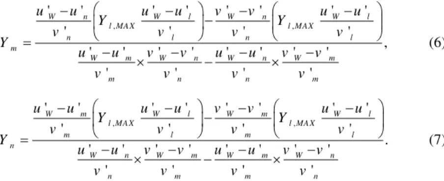
2.3 Determination of the optimal converting point of CT conversion for SSL complied with ANSI C78. 377
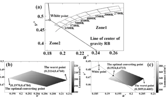
The ANSI C78. 377 gauges the eight CT (2700K, 3000K, 3500K, 4000K, 4500K, 5000K, 5700K, 6500K) ranges for indoor SSL application. This standard gauges each CT as a quadrangle. The color points of the same CT quadrangle represent the same color perception for human eyes. However, there are many color points in the range of CT quadrangle. Which color point is the optimal converting point? As shown in Fig. 3(a), the line of center of gravity may or may not intersect with the CT quadrangle. For example, the CT quadrangle A intersects with the line of center of gravity, whereas the quadrangle B does not. When the CT quadrangle A is chosen to be the target CT, the point c is the optimal converting point of the range of CT quadrangle A. As shown in Fig. 3(b), because the expanded color gamut from the reference white point (W) first meets the point c, the area of the expanded color gamut is smaller than that meeting other color points in the range of CT quadrangle A. (for example,
when the expanded color gamut meets the point c’, the area is bigger than it meets the point c.) When the CT quadrangle B is chosen to be the target CT, the point d is the optimal converting point of the range of CT quadrangle B. Because the point d is first met by the expanded color gamut from the reference white point, the color gamut area is the smallest under the range of CT quadrangle B. The maximal luminance of the optimal converting point can be obtained from the Eqs. (6) and (7). Hence, when the CT quadrangle intersects with line of center of gravity, the optimal converting point of the target CT is the intersection between the line of center of gravity and the edge line of CT quadrangle. When the CT quadrangle does not intersect with line of center of gravity, the optimal converting point is the corner point of the CT quadrangle which is first met by the expanded color gamut from the reference white point.
Fig. 3. The optimal converting points of the CT quadrangle A and CT quadrangle B. (a) The point c is the optimal converting point of CT quadrangle A. The point d is the optimal converting point of CT quadrangle B. (b) The local magnified picture of (a) explains that c is the optimal converting point of quadrangle A.
3. Simulations and discussion
3.1 Simulation of display application
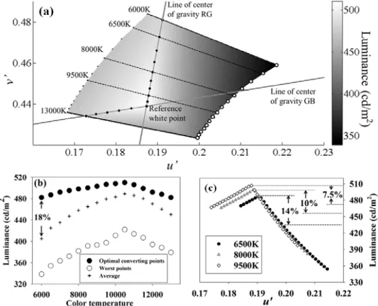
In order to prove the reliability of the proposed method for determining the optimal converting point of CT conversion, this simulation took 31 simulated points on the isotemperature line of each target CT. The simulated target CTs were from 6000K to 13000K. In order to keep chromaticity [2], the 31 simulated points were retained in ∆u’v’ = ± 0.04 between endpoint of isotemperature line and Planckian locus. The parameters of simulation were measured from the 30 inch LCD (Panasonic, TC-30MTF). The u’v’ chromaticity coordinates of the tri-primaries, R, G, and B were respectively (0.4490, 0.5241), (0.1139, 0.5556), and (0.1627, 0.1688). The luminance of the tri-primaries, R, G, and B were respectively 108.4 cd/m2, 347.08 cd/m2, and 56.41 cd/m2. The reference white point of the display was 10500K. Figure 4(a) shows the variation of luminance and chromaticity coordinates of simulated points of target CTs from 6000K to 13000K. The optimal converting points (solid circles) of each target CT were located on the intersection between line of center of gravity and isotemperature line. The worst points (hollow circles) were located on the endpoint of each isotemperature line. This was because when the color gamut expanded from the reference white point to the endpoint of isotempature line, the area of color gamut was bigger than it expanding to others point on the isotemperature line. For example, when the
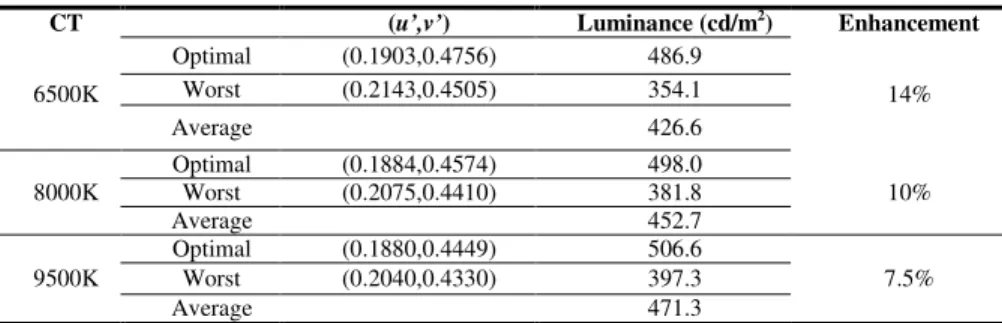
reference white point was converted to the color point on the 9500K isotemperature line, the luminance of black solid circle was more than hollow circle. Moreover, when the target CT was lower than the 10500K (reference white point), the optimal converting point of target CT was the intersection between line of center of gravity RG and the isotemperature line of target CT. When the target CT was higher than the 10500K, the optimal converting point was the intersection between line of center of gravity GB and the isotemperature line of target CT. The results were in accordance with the proposed method of this paper. Figure 4(b) shows the luminance of optimal converting points, worst points, and average value of all target CTs. The enhancement of the luminance was defined as “(optimal-average)/average”, where the optimal represented the optimal converting point and the average represented the average luminance value of 31 simulated color points of each CT. The maximal enhancement of luminance was on 6000K with 18%. The minimal enhancement of luminance was on 10500K with 6%. Hence, when the target CT was close to the reference white point (10500K) of the display, the enhancement of the luminance was limited. This was because the luminance of target CT was already close to the luminance of the reference white point of the display. Figure 4(c) shows the luminance of 31 simulated points of three CT modes (6500K, 8000K and 9500K) usually using by the display. Table 1 lists the results of these three useful CT modes. From the results, when people used the proposed method to implement the CT conversion of these three CT modes, the enhancement of luminance was 14%, 10%, and 7.5%, respectively.
Fig. 4. (a) The variation of luminance and chromaticity coordinates of the 31 simulated points on isotemperature line of all target CTs. The black solid circles and hollow circles individual represent the optimal converting points and worst points of each target CT. (b) The luminance of optimal converting points, worst points, and average value of each target CT. (c) The enhancement of luminance of three useful target CTs.
Table 1. The simulated results of three usually used CT modes of display CT (u’,v’) Luminance (cd/m2) Enhancement
6500K Optimal (0.1903,0.4756) 486.9 14% Worst (0.2143,0.4505) 354.1 Average 426.6 8000K Optimal (0.1884,0.4574) 498.0 10% Worst (0.2075,0.4410) 381.8 Average 452.7 9500K Optimal (0.1880,0.4449) 506.6 7.5% Worst (0.2040,0.4330) 397.3 Average 471.3 3.2 Simulation of SSL application
For the SSL case, the simulation was based on the conditions with luminance of tri-primaries
YR = 42.3 cd/m2, YG = 428.8 cd/m2 and YB = 5.1 cd/m2. The u’v’ chromaticity coordinates of
the tri-primaries, R, G, and B were respectively (0.5509, 0.5168), (0.1420, 0.5741), and (0.2002, 0.0339). These parameters were based on the LED product specification (RED POWER CO., LTD., u42RGBC2B-016). The ANSI C78. 377 gauged eight CTs for application. Figure 5(a) shows the simulated results of these eight CTs. As shown in Fig. 5(a), only the 6500K CT quadrangle intersected with the line of center of gravity. Hence, the simulation used the 5700K and 6500K to be the examples. We individual took 10000 points in these two CT quadrangles for simulation. The chromaticity coordinate of four corners of 5700K and 6500K quadrangles were according to the gauge of ANSI C78. 377. As shown in Fig. 5(b), when the color points were located away from the reference white point, the luminance of the color points must be decreased. This was because when the expanded color gamut from reference white point met the distant color point, the area of expanded color gamut was bigger than it meeting others color points. Therefore, the optimal converting point was located on the leftmost point of the quadrangle with the luminance of 226.4316 cd/m2. The worst point was located on the rightmost point of the quadrangle with the luminance of 188.0372 cd/m2. As shown in Fig. 5(c), the optimal converting point was the first intersection between line of center of gravity and edge line of 6500K CT quadrangle. The luminance of optimal converting point was 395.2242 cd/m2. The worst point was located on the rightmost point of the quadrangle with the luminance of 296.9473 cd/m2. The enhancement of luminance was defined as “(optimal-average)/average”, where the average was the average luminance value of 10000 points and optimal was the luminance of optimal converting point. The enhancement of luminance of 5700K and 6500K was 14.2% and 23.6%, respectively. Therefore, when the line of center of gravity intersected with the edge line of the CT quadrangle, the optimal converting point was the first intersection on the edge line of CT quadrangle. When the CT quadrangle did not intersect with the line of center of gravity, the corner point of CT quadrangle which was closest to the reference white point was the optimal converting pint. The results were in accordance with the proposed method of the article.
Fig. 5. (a) The eight CT quadrangles in the u’v’ chromaticity coordinate. (b) The variation of luminance of 5700K CT quadrangle. (c) The variation of luminance of 6500K CT quadrangle. 4. Experiment and discussion
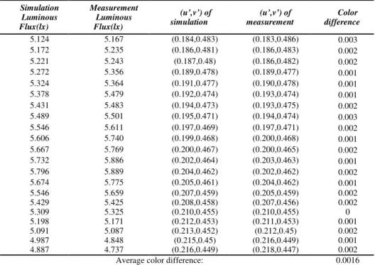
For the purpose of verifying the practicability of the proposed method, the experiment simulated 1050 points on the isotemperature line of 6500K and measured 21 points of the 1050 points. Figure 6(a) presents the experimental setup. The gray level signal was generated using a computer with a DVI output chip (nVidia 7600gs). In order to increase the accuracy of measurement, the gray level signal was measured using a spectrum meter (SphereOptics SMS-500) in units of luminous flux. In order to stabilize the backlight, the monitor was preheated for around 45 minutes in the darkroom. The fiber (OceanOptics) was placed at the center of the 17” LCD (Viewsonic VX710) monitor to prevent light leakage. The reference white point of the 17” LCD was 6100K. The experiment chose the 6500K to be the target CT. The 1050 simulated points was chosen in the range of ∆u’v’ = ± 0.04 between the endpoint of isotemperature line and the Planckian locus. In order to make the 21 measured points had the same chromaticity coordinates as the simulations, the experiment tuned luminance of the tri-primaries (R, G and B) of the display. Figure 6(b) shows the results of 1050 simulated points and 21 measured points. The values were listed on Table 2. The 13th measured point on the 6500K isotemperature line was the optimal converting point with luminous flux of 5.889 lx. The point was also the optimal converting point of the simulation. The 21th measured point was the worst point with luminous flux of 4.737 lx. The point was also worst point of simulation. The average luminous flux of the 21 points was 5.162 lx. The enhancement of luminous flux was about 14.08%. The optimal and worst points were the same in the simulation and experiment. Since the target CT was close to the reference white point (6100K) of the 17” LCD, the enhancement of luminous flux was only about 14.08%. The color difference between the simulated points and measured points did not exceed 0.003. Hence, the experimental results were credible. The color difference between the simulated and measured points was caused by the luminance of quantization effects. Moreover, the leakage of light from displays also caused a tiny error.
Fig. 6. (a) The setup of experiment. (b) The results of experiment on 6500K isotemperature line.
Table 2. The experimental results of chromaticity coordinates and luminous flux on 6500K isotemperature line Simulation Luminous Flux(lx) Measurement Luminous Flux(lx) (u’,v’) of simulation (u’,v’) of measurement Color difference 5.124 5.167 (0.184,0.483) (0.183,0.486) 0.003 5.172 5.235 (0.186,0.481) (0.186,0.483) 0.002 5.221 5.243 (0.187,0.48) (0.186,0.482) 0.002 5.272 5.356 (0.189,0.478) (0.189,0.477) 0.001 5.324 5.364 (0.191,0.477) (0.190,0.478) 0.001 5.378 5.479 (0.192,0.474) (0.193,0.474) 0.001 5.431 5.483 (0.194,0.473) (0.193,0.475) 0.002 5.489 5.501 (0.195,0.471) (0.194,0.474) 0.003 5.546 5.611 (0.197,0.469) (0.197,0.471) 0.002 5.606 5.740 (0.199,0.468) (0.200,0.468) 0.001 5.667 5.769 (0.200,0.467) (0.200,0.465) 0.002 5.732 5.886 (0.202,0.464) (0.203,0.463) 0.001 5.796 5.889 (0.204,0.462) (0.202,0.462) 0.002 5.674 5.775 (0.205,0.461) (0.204,0.462) 0.001 5.546 5.659 (0.207,0.459) (0.205,0.459) 0.002 5.429 5.425 (0.208,0.458) (0.207,0.456) 0.002 5.309 5.325 (0.210,0.455) (0.210,0.455) 0 5.198 5.171 (0.212,0.453) (0.211,0.453) 0.001 5.091 5.087 (0.213,0.452) (0.212,0.45) 0.002 4.987 4.848 (0.215,0.45) (0.216,0.449) 0.001 4.887 4.737 (0.216,0.449) (0.218,0.447) 0.002
Average color difference: 0.0016
5. Conclusions
The CT conversion is an important issue for lighting and display. Until now, there is no any method to find the optimal converting point of the target CT for the CT conversion. This paper proposes the effective methods for obtaining optimal converting point of CT conversion. For display application, the method is to find the intersection between the line of center of gravity and isotemperature line of the target CT. For SSL application, this paper proposes two methods for determining the optimal converting point of the range of CT quadrangle. When the CT quadrangle intersects with the line of center of gravity, the optimal converting point is the intersection between the line of center of gravity and the edge line of the CT quadrangle. When the CT quadrangle does not intersect with the line of center of gravity, the optimal converting point is the corner point of the CT quadrangle first meeting by
the expanded color gamut from the reference white point. The improvement of luminance for CT conversion is reported in this study. Hence, when people want to implement the CT conversion for display or SSL, these methods can help them to determine the optimal converting point of the target CT. Our future research will apply the method and theory to multi-primaries displays.
Acknowledgments
This paper is particularly supported by the “Aim for the Top University Plan” of the National Chiao-Tung University and Ministry of Education, Taiwan, R.O.C., the National Science Council of Taiwan (Contracts No. NSC 101-2220-E-009-032, NSC 101-2623-E-009-006-D, NSC 101-2218-E-039-001) and the Chung-Shan Institute of Science & Technology under contracts XV00E19P295 and CSIST-442-V302, and Delta Electronics Incorporation (Contract No. NCU-DEL-101-A-04). The authors want to thank them for providing experimental assistance and related information.