Controller Parameterization for Disturbance
Response Decoupling: Application to
Vehicle Active Suspension Control
Malcolm C. Smith, Fellow, IEEE, and Fu-Cheng Wang, Student Member, IEEE
Abstract—This paper derives a parameterization of the set of all stabilizing controllers for a given plant which leaves some prespecified closed-loop transfer function fixed. This result is motivated by the need to independently shape several different disturbance transmission paths in vehicle active suspension control. The result is studied in the context of quarter-, half-, and full-car vehicle models, to derive appropriate controller structures. A controller design is carried out for the full-car case and simulated with a nonlinear vehicle dynamics model.
Index Terms—Active suspension, controller parameterization, disturbance response decoupling, , loop-shaping, vehicle dynamics.
I. INTRODUCTION
T
HIS paper studies the problem of control system design when there are independent performance goals for sev-eral disturbance transmission paths. We are motivated by the problem of vehicle active suspension control where a key fea-ture is the need to insulate the vehicle body from both road ir-regularities and load disturbances (e.g., inertial loads induced by braking and cornering). It is well known that these are con-flicting requirements when passive suspensions are used, but the conflict may be removed when active control is employed with appropriate hardware structure, e.g., choice of sensor lo-cation, number, and type. Once a suitable hardware structure is selected, there remains the problem of designing the controller to achieve satisfactory responses for all of the disturbance trans-mission paths. It is this latter problem that is the main subject of this paper. To this end, we consider the problem of parameter-izing the set of all stabilparameter-izing controllers for a given plant which leaves the transfer function for a given disturbance transmission path the same as when some nominal stabilizing controller is employed. In this way, the design for each disturbance path can be carried out successively, providing there is sufficient freedom to adjust the responses independently.A. Vehicle Active Suspension Control
The use of active suspension on road vehicles has been considered for many years [8], [15], [17], [20], [26]. A large
Manuscript received November 30, 2000; revised July 31, 2001. Manuscript received in final form October 23, 2001. Recommended by Associate Editor M. Jankovic.
The authors are with the Department of Engineering, University of Cambridge, Cambridge CB2 1PZ, U.K. (e-mail: [email protected]; [email protected]).
Publisher Item Identifier S 1063-6536(02)01768-2.
number of different arrangements from semiactive to fully active schemes has been investigated [2], [16], [25], [27]. There has also been interest in characterizing the degrees of freedom and constraints involved in active suspension design. Constraints on the achievable response have been investigated from “invariant point,” transfer-function, and energy/passivity points of view in [7], [9], [10], [18], [19]. In [18], a complete set of constraints was derived on the road and load disturbance response transfer-functions and results on the choice of sensors needed to achieve these degrees of freedom independently were obtained for the quarter-car model (see [4] for generalization of these results to half- and full-car models). In [19] it was shown that the road and load disturbance responses could not be adjusted independently for any passive suspension applied to a quarter-car model.
The need to design the road and load disturbance responses independently has been considered elsewhere in the active sus-pension literature. For example, in [15] a hardware and sensing arrangement was devised so that the feedback part of the scheme would not affect the response to road disturbances, which were designed to be suitably soft by means of passive elements in the scheme. In [24], [25] the actuator was placed in series with a spring and damper, which were chosen to give a suitably soft re-sponse to road irregularities in the absence of a feedback signal. A controller structure using a filtered combination of the sensor measurements was then selected so that the road disturbance responses were unaffected by the feedback. The present paper represents a continuation of this idea by finding in general the required controller structure to achieve this property for any set of measurements.
In active suspension design for full-car models, it has been found advantageous to decompose the motion into bounce, pitch and roll components for the vehicle body and additionally warp for the wheels in contact with the road [6], [12], [13], [19]. This paper will also exploit such transformations, at least to a par-tial extent. In the full-car case we will exploit symmetry to de-compose into the bounce/pitch and roll/warp half-cars. In the half-car case we will use our results to determine the feedback structure to allow road and load disturbances to be shaped inde-pendently and discuss the simplicity assumptions which allow a further decomposition of the half-car into two quarter-cars.
B. Controller Parameterization
The idea of parameterizing all stabilizing controllers in a linear feedback system is a standard one [28], [30]. The extension of this idea to two-degree-of-freedom schemes 1063-6536/02$17.00 © 2002 IEEE
(which allows the response to reference commands and the return ratio of the feedback path to be optimized independently) is also standard [21], [29]. The generalization to additional degrees-of-freedom to include some exogenous disturbances has also been considered [14]. The parameterization of all sta-bilizing controllers which leaves some prespecified closed-loop transfer function fixed, as considered in this paper, represents a continuation of these ideas and techniques.
Our approach makes use of algebraic properties of the ring of stable, proper rational functions [21]. To facilitate the parame-terization at the required level of generality we will introduce the idea of left and right normal rank factorizations of a rational matrix (Definition 1).
C. Outline of Paper
Section II sets up in generality the problem of parameter-izing all stabilparameter-izing controllers which leave some prespecified closed-loop transfer function fixed. Our basic results, which characterize the required structure of the Youla -parameter, are given in Theorems 1 and 2. Section III considers the standard quarter-car model employing a “Sharp” actuator with various choices of measured variables. The required controller structures to leave the road disturbance responses the same as in the passive case are derived using the results of Section II. Section IV considers a simple half-car model with acceleration and strut deflection measurements, and again derives the con-trol structure required to keep the road disturbance responses the same as in the passive case. “Simplicity” conditions which allow the design to be carried out for two separate quarter-cars are presented. Section V considers a simple linearized full-car model and shows how this may be separated into two half-car models under a mild symmetry assumption. Section VI presents a design for the full-car model with acceleration and strut de-flection measurements. The bounce/pitch half-car is treated according to the theory in Section IV. The roll and warp modes are each treated as quarter-cars with the warp mode being handled in a special way. The controller design is simulated with a nonlinear vehicle model using the multibody simulation package AutoSim.
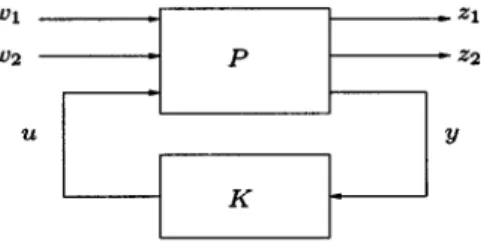
II. CONTROLLERPARAMETRISATIONRESULTS We consider the LFT (linear fractional transformation) model in Fig. 1, where the Laplace transfer function of the generalized plant is partitioned as
and further partitioned conformably with the disturbance signals as
(1)
where , , , , ,
at any time instant denotes the Laplace transform of etc. Weconsider the problemof parameterizing all stabilizing
controllers which leave (the transfer function from to ) the same as for some given stabilizing controller .
Let be the right and left coprime
factorizations of over . Then all stabilizing controllers can be parameterized by
(2) (3)
for where , , , are matrices with
ele-ments in which satisfy the Bezout identity
For our first result (Theorem 1) it is convenient if the factor-izations are chosen so that corresponds to the desired
stabilizing controller, i.e., . (This
as-sumption will be relaxed in the corollary to Theorem 2.) The results we will establish in this section make use of cer-tain algebraic properties of the set , namely its ring struc-ture. The reader is referred to [21] for the necessary background on this topic. Here we will be content to recall a few facts. The set has the property of being a Euclidean domain with de-gree function defined by the total number of zeros of the element in the closed right half plane and at infinity (counting multiplic-ities). The invertible elements in are called units, and are the elements with degree equal to zero. A matrix
is called unimodular if it has an inverse whose elements belong to , or equivalently, if its determinant is a unit in .
The normal rank of a matrix , denoted normal
rank , is the maximum rank of for any which
is not a pole. Equivalently, the normal rank is equal to the rank for almost all . We now introduce a type of matrix factor-ization which will be useful in proving the subsequent results.
Definition 1: Let be a matrix with elements in . is said to have a left normal rank factorization (lnf) if there exist
matrices and over with of full column
normal rank and unimodular such that . is said to have a right normal rank factorization (rnf) if there exist
ma-trices and over with of full row normal
rank and unimodular such that .
Lemma 1: For any , there exists an lnf and an rnf of .
Proof: See the Appendix.
We return to the problem of parameterizing all stabilizing controllers which leave the transfer function the same
as when the controller is applied. From
[5], the closed-loop transfer function in Fig. 1 can be expressed as
(4)
Fig. 1. Generalized model in LFT form.
Thus the problem reduces to parameterizing all stabilizing con-trollers which leave . These are characterized
by all such that ,
where and . We now introduce
an lnf of and an rnf of as follows:
(5) (6)
where , , ,
, and are the normal rank of and
re-spectively. Note that and are also the normal rank of and , respectively. Furthermore, we have the inequalities
, .
Theorem 1: Consider any stabilizable in the configuration of Fig. 1. All stabilizing controllers such that the closed-loop
transfer function are given by expressed
in the form of (2) and (3) with
(7)
for and , and
defined from the lnf and rnf factorizations (5) and (6), ,
are chosen such that and are unimodular, and
is a partition of
Proof: See the Appendix.
The control structure given in (7) is arrived at by completing the matrix to a unimodular matrix and then extracting from the resulting matrix inverse. Since and the completion are not unique then neither is . It will be useful to characterize this nonuniqueness in terms of the parameterization of the set directly. This is done in the fol-lowing lemma.
Lemma 2: Given two sets and
where , are full
row normal rank, then
1) if and only if is a left multiple of over , i.e., there exists a such that .
2) if and only if there exists a unimodular matrix
such that .
Proof: See the Appendix.
Throughout this paper the vehicle dynamics examples will satisfy some special assumptions on the open-loop plant. This
allows the controller parameterization of Theorem 1 to take a simplified form, and it turns out that a further useful structural simplification can then be made. It will be convenient to summa-rize these simplifications in the theorem below, which will then be applied directly throughout the paper. (The first two special assumptions on the open-loop plant arise because of some pas-sive elements in the suspension system which ensure that the road disturbance responses are satisfactory without any feed-back control. The third assumption is a rather technical one which says that the number of outputs to be left invariant is no smaller than the number of actuators and that this transmission path has full normal rank.)
Theorem 2: Let (i) be (open-loop) stable, (ii) ,
(iii) .
1) There exists such that all stabilizing
controllers which give can be
param-eterized as
(8)
for .
2) A particular for which (8)
param-eterizes all stabilizing controllers such that
can be calculated as follows: choose ,
, , , , ,
and , define from the rnf (6), and cal-culate , as in Theorem 1.
3) Consider any such that
parameterizes all stabilizing controllers which give . Then there exist a unimodular matrix
such that , where is defined in 2).
4) Let be defined in 2) and let be any stabilizing con-troller for . Then is a stabilizing controller
for for which .
5) Let be defined in 2) and consider any stabilizing
con-troller for for which . Then we
can write , where is a stabilizing controller
for .
Proof: See the Appendix.
Corollary 1: Let conditions (i) and (iii) of Theorem 2
hold and suppose that for some
. Then all stabilizing controllers which leave the same as when is applied can be parameterized as
(9)
for some and defined in Theorem 2 (2).
Proof: See the Appendix.
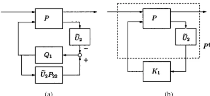
The controller structure given in (8), which is a special case of the general parameterization given in Theorem 1, may be rep-resented in the block diagram form shown in Fig. 2(a). Theorem 2(4, 5) shows that the essential feature in this controller struc-ture is the presence of as the rightmost term in (8). This is illustrated in the block diagram Fig. 2(b) where may be any stabilizing controller for the transformed plant .
(a) (b) Fig. 2. (a) General controller structure. (b) Equivalent controller.
Fig. 3. The quarter-car model.
III. THEQUARTER-CARMODEL
A. The Quarter-Car With Two Measurements
We begin with the quarter-car model of Fig. 3 where the sprung and unsprung masses are and and the tire is mod-eled as a linear spring with constant . The suspension consists of a passive damper of constant in parallel with a series com-bination of an actuator and a spring of constant (sometimes referred to as a “Sharp” actuator [27]). Following [16] the actu-ator is modeled so that the relative displacement across the ac-tuator will be a low-pass filtered version of the acac-tuator’s com-mand signal, i.e.,
(10) As in [16], we use a second-order filter to represent the actuator dynamics
(11) The external disturbances are taken to be a load and a road displacement , and the measurements are taken to be and
. The dynamic equations of the model are given by (12) (13) where
(14) (15) We wish to parameterize all controllers which leave the trans-mission path from the road disturbance to and the same as in the open-loop, i.e., with . This assumes that and are chosen to give satisfactory responses for this transmission
path. In effect, this gives the choice of . We now write
the system in the form of Fig. 1 with , ,
, , equals the actuator command
signal as in (10) and omitted. The corresponding dimensions
are , , , . Equation
(1) then takes the form
with the transfer functions being given by
(16) (17)
where and
(18) As expected, all roots of are in left-half plane, which can be confirmed by the Routh–Hurwitz criterion.
We now observe that , which has normal rank
equal to one, i.e., . Since is open-loop stable and , the conditions of Theorem 2 are satisfied. We can then apply Theorem 2(2) to find the matrix which defines the required control structure. Following the definitions in Theorem 2(2) we first find
which has normal rank equal to one, i.e., . Hence we can select
for any , to give a rnf of . We can choose to
complete a unimodular matrix as follows:
which gives and
(19) Thus, all stabilizing controllers which leave the same as in the open-loop can then be expressed as shown in Fig. 4 where
(20) for or equivalently is any stabilizing controller
Fig. 4. Controller structure for the quarter-car with two feedbacks.
Example 1: We now apply the above result to a specific case
in which we make the suspension stiff to load disturbances but soft to road disturbances. We select the following parameters for the quarter-car model as in [19] which correspond roughly
to a small saloon car [3]: kg, kg,
kN/m. We choose rad/s and as
the parameters for the actuator dynamics. We also choose kN/m, kNs/m as the spring-damper coefficients which we consider to give a suitable “soft” response from the road disturbances in the passive implementation. It is now required to design the active controller to achieve desirable responses from the load disturbances.
A simple approach is to take to be constant in (20) and to minimize the steady-state response from load disturbances to sprung mass position. A straightforward calculation shows that which can be made to
equal zero when . The step responses
for the passive and active suspensions are shown in Fig. 5, which clearly illustrates the zero steady-state response to loads achieved by the active controller. The following closed-loop
eigenvalues were obtained: 3.00, 3.95, ,
83.97, .
As a second approach we can employ the loop shaping design procedure [11], [30] to the plant . We select a
weighting function , so that the
open-loop loop shape, , has a gain crossover fre-quency at about 44 rad/s, somewhat below the actuator cutoff frequency of 100 rad/s. The use of a lag compensator in allows the gain to be increased relatively at low frequencies in order to achieve a smaller value of . This choice of weighting function gives a stability margin of 0.3864. The final controller takes the form (see Fig. 4) where
which has been reduced to third order by balanced truncation. For this controller the step response from to is shown in Fig. 6, which exhibits an improved transient response in comparison to Fig. 5 but inferior steady-state behavior. The following closed-loop eigenvalues were obtained: 3.95,
, , 83.97, ,
.
At this point it is instructive to compare the control struc-ture shown in Fig. 4 with a scheme presented by Williams et
Fig. 5. Passive suspension (Q = 0, solid) and active suspension (Q = 1:08, dashed).
Fig. 6. Passive suspension (solid) and active suspension using H loop shaping design (dashed).
Fig. 7. Controller structure of Williams et al.
al. in [25]. The stated aim of their controller is to provide a
rapid closed-loop levelling system which does not respond to unwanted road disturbances, and this is achieved “by filtering and summing the sprung mass acceleration and suspension displacement signals to eliminate the effects of the road in-puts.” A block diagram of the scheme in [25] is shown in Fig. 7 where is a phase lead compensator. Although the damper is placed in series with the actuator this is not an essential difference. It may be observed that the ratio between
the two filters and is equal to so the
scheme operates in a similar way to that of Fig. 4. In fact it can be shown that, if the denominators in and are both replaced by , and is any stabilizing controller, then the scheme parameterizes all controllers which leave the
road disturbance responses the same as in the open loop. Thus the scheme lacks full generality only by virtue of the fact that the filters and have an extra order of roll-off at high frequency, which is a minor difference since it may be useful to provide some high-frequency roll-off in in practice.
We point out that our chosen scheme, as well as the approach of [25], assumes that the ride performance is satisfactory with . If this is not the case, a controller may first be design to give any other desired road disturbance responses. Thereafter, Corollary 1 may be utilized to shape the load distur-bance responses as well.
Finally, it is useful to comment on the full set of performance requirements that are usually considered in suspension design. In addition to the sprung mass position as a function of road disturbances, which can be analyzed with regard to driver com-fort, there are also issues such as tire normal loads (i.e., tire de-flection) and rattle space (i.e., strut dede-flection). It was shown in [7] that if the transfer function from to is determined, then there is no additional freedom left in the road disturbance transmission path, i.e., the transfer functions and can be deduced directly. A similar fact was shown in [18] for the load disturbance transmission path. Thus, in the above approach to active suspension design, it is assumed that for each disturbance transmission path that is being dealt with, all the relevant factors (e.g., comfort, tire loads, suspension de-flection) are taken account of together.
B. The Quarter-Car With Three Measurements
We continue to illustrate our basic theory by considering the quarter-car model with the additional measurement . We now write the system in the form of Fig. 1 with
and all other variables the same as in Section III-A. The general plant of (1) then has , the same as (16), (17) and
where , are given in and before (18).
As before we wish to parameterize all controllers which leave the transmission path from the road disturbance to and the same as in the open-loop, i.e., with , which assumes that and are chosen to give satisfactory responses for this transmission path. We can check that the conditions of Theorem 2 again hold, so that we can follow the procedure to obtain the required controller structure.
Following the definitions in Theorem 2(2) we find that
Fig. 8. Controller structure for the quarter-car with three feedbacks. which gives . Hence we can select
where is any second-order Hurwitz polynomial, to give a
rnf of . We can choose to complete a
unimodular matrix to give with
(21) Thus, all stabilizing controllers which leave the same as in the open-loop can then be expressed as shown in Fig. 8 where
(22) for any or equivalently is any stabilizing con-troller for (see Theorem 2).
1) Alternative Controller Structures: As pointed out in
Lemma 2 the exact form of in (21) is not unique. Let us suppose that we prefer a structure with
where , are strictly proper, motivated by a prefer-ence to use low-pass filters for the acceleration signals and while keeping the strut deflection unfiltered. For given by
(21) the identity implies that
and
We can see that fails to be unimodular as required by Theorem 2(3). Moreover, it is straightforward to show
that the set is equal to the set
, i.e., the full parameter-ization but with the first element in being strictly proper.
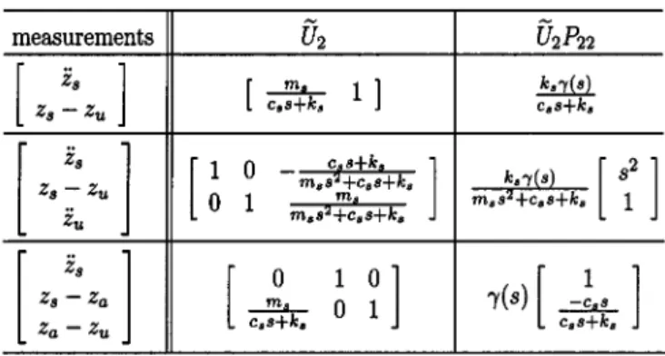
TABLE I
THEU STRUCTURES AND THETRANSFORMEDPLANTS OF THE QUARTER-CARMODELWITHVARIOUSMEASUREMENTS
Thus a controller parameterization with replaced by does not give all possible stabilizing controllers which leave the road disturbance responses the same as in the open-loop (see Lemma 2 and Theorem 2). However, the restriction of the -parameter amounts only to an increased roll-off requirement of the controller at high frequency.
Referring to Fig. 8, let us consider another possible controller structure
where , are strictly proper. The identity now implies that
and
Since is unimodular, then can be replaced by in Fig. 8 to give a parameterization of all stabilizing controllers [Theorem 2(3)].
C. Quarter-Car Control Structures and Design
For direct controller design using Theorem 2, it is instruc-tive to compute for the given choice of measurements. Table I shows for three different cases. It is interesting that takes a particularly simple form, which is indepen-dent of the sprung and unsprung masses, in the case when the feedback signals and are used, which means that the controller design would be rather simple in this case.
IV. THEHALF-CARMODEL
In this section, we shall apply the controller parameteriza-tion method to the half-car model shown in Fig. 9. As in the quarter-car model, the actuators and are modeled so that the relative displacement across each is equal to a low-pass fil-tered version of the actuator’s command signal, i.e.,
(23) (24)
Fig. 9. The half-car model.
where is defined as in (11). The linearized dynamic equa-tions can be expressed as follows:
(25) (26) (27) (28) where the passive suspension forces , , and the tire forces
, are given by
We now write the system in the form of Fig. 1 with
, , ,
where ,
are strut deflections, as in (23), (24) and omitted. As before we wish to parameterize all controllers which leave the transmission path from the road
disturbances to the same as in the
open-loop, i.e., with , which assumes that ,
, and are chosen to give satisfactory responses for these transmission paths. We can check that the conditions of Theorem 2 again hold, so that we can follow the procedure to obtain the required controller structure.
Following the definitions in Theorem 2(2) we can choose a and , where is any third-order Hurwitz polynomial, to give a rnf of , and complete this
to a unimodular matrix with to give
(29)
We observe that “constructs” two combinations of measure-ments, each of which is a suspension deflection plus a low-pass filtered version of a sum of the two acceleration signals. A block diagram of this control structure is shown in Fig. 10.
Fig. 10. Controller structure(U ) for the half-car model.
For direct controller design using the transformed plant in Fig. 2(b), it is interesting to note that takes a particularly simple form in the half-car case when is determined by (29), namely
(30) This fact will be exploited in the design example for the full-car model in Section VI.
A. Decoupling by Simplicity
Under certain conditions, the half-car model can be struc-turally decoupled into two quarter-cars, and in such cases it is useful to exploit the simplified structure. In [19] and [22], as-sumptions such as kl-simplicity were used, in a mechanical net-work setting, to perform energy-preserving transformations of the external disturbance variables to achieve decoupling. In our setting we will need to use a similar transformation on all of the system variables (but will not necessarily be able to respect the energy-preserving property). For the half-car model shown in Fig. 9, we define it as simple if the following equation holds:
(31) Note that half-car roll models are typically symmetric (i.e., , etc.) so that (31) holds automatically in this case. Condition (31) may sometimes be satisfied also for half-car pitch models. We introduce a transformation matrix as follows:
(32) and define
where may represent any of the following variables: , , , or , and the subscripts and represent the bounce and rotation modes, respectively.
Under the assumption of simplicity, we can then rewrite (23)–(28) as follows:
(33) (34)
(35)
TABLE II
DECOUPLEDHALF-CAR BYSIMPLICITY
(36)
(37)
(38) Comparing with (10), (12) and (13), we find that (33), (35) and (37) represent a bounce quarter-car, and (34), (36) and (38) represent a rotation quarter-car, which are decoupled from each other. The relevant correspondences between variables is sum-marized in Table II. Furthermore, we can show that, in order to arrive at a decoupled form for (35) and (36) (e.g., being ab-sent from (35) etc), then we need both (31) to hold and for to be defined by (32) up to scalar multiplication of each row.
V. THEFULL-CARMODEL
In this section we shall introduce a standard full-car model with a similar suspension strut arrangement at each wheel-sta-tion to the quarter- and half-car cases in Figs. 3 and 9. We assume a left-right symmetry which allows a decoupling of the full-car model into two half-cars, namely the bounce/pitch and roll/warp half-cars. In preparation for a controller design in Section VI we will highlight the special form of the warp quarter-car, which has no “sprung mass dynamics.”
A. The Dynamic Equations
Referring to Fig. 11, the actuators are again modeled so that the relative displacement of each is equal to a low-pass filtered version of the actuator’s command signals, i.e.,
where is defined as in (11). The linearized dynamics of the full-car can be expressed as
Fig. 11. The full-car model. (40) (41) (42) (43) (44) (45) where the passive suspension forces and the tire
forces are given by
(46) (47)
for , , and the strut deflections are
B. Symmetric Transformation
Since the full-car model is symmetric, we can decouple it into two half-car models. First, we introduce a transformation matrix
:
(48)
such that
(49) where may represent any of the following variables: , , , strut deflection or actuator command signal , while the
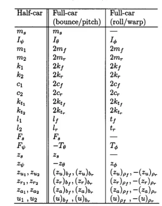
TABLE III
DECOUPLED(SYMMETRIC) FULL-CAR
subscripts , represent the front and rear bounce components , represent the front and rear roll components.
1) Bounce/Pitch Half-Car: After applying the trans-formation, (39), (40), and (42)–(45) can be rearranged as follows:
It can be observed that the above equations take the same form as (25)–(28) under the transformations listed in the first column of Table III. To decouple into two quarter-cars requires a simplicity assumption
TABLE IV
DECOUPLEDROLL ANDWARPMODES OF THEFULL-CAR BYSIMPLICITY
2) Roll/Warp Half-Car: After applying the transforma-tion, (41)–(45) can be rearranged as follows:
We observe that one equation is missing in this half-car com-pared to (25)–(28). This is because the chassis is modeled as being infinitely stiff under torsion, so that there is no dynamic equation corresponding to warp dynamics of the car body. However the above three equations do take a similar form to (26)–(28) under the transformations listed in the second column of Table III.
As in the half-car case, under the assumption of simplicity (51) and the transformation
(52) such that
(53) where can be , or , strut deflection or actuator com-mand signal , the roll/warp half-car can be further decoupled into roll and warp quarter-cars under the mapping illustrated in Table IV.
VI. A DESIGNEXAMPLE FOR THEFULL-CARMODEL In this section, we shall synthesize an active controller for a specific full-car model. As in Section V, the model is chosen to be left-right symmetric which allows a decoupling into the
bounce/pitch and roll/warp half-cars. Our design approach for
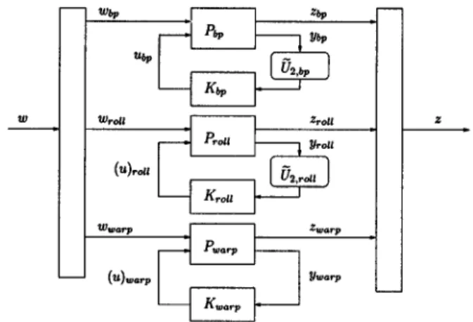
Fig. 12. Control scheme for the full-car model.
the bounce/pitch half-car will make use of the theory outlined in Section IV. The approach for the roll/warp half-car will make use of a simplicity assumption which allows it to be decoupled into the two corresponding quarter-cars, namely the roll and
warp quarter-cars. The roll quarter-car will be treated in the
same way as the quarter-car of Section III-A. As pointed out in Section V-B2, the warp quarter-car has a different form than the standard quarter-car in that the “sprung mass” is effectively infinite. Furthermore, in warp motion there is good reason to use the active controller to make the road disturbance responses even softer than they would be with the default passive param-eter settings. Thus the warp mode will be handled in a different way to the other three modes.
For the controller design the available measurements are as-sumed to be , , , , , , and . The control struc-ture will be chosen to have three independent loops, consisting of the roll quarter-car, the warp quarter-car, and bounce/pitch half-car controllers. This scheme is shown in Fig. 12, where the signals are defined as follows:
(54)
(55)
and the subscripts , , , and are defined as in (49) and (53).
The following parameters will be used for the full-car model which are similar to typical parameters for a sports car [3]:
kg, kg m , kg m , m,
m, m, kN/m,
Fig. 13. Step responses ofT andT : passive (solid) and active control (dashed).
the previous examples, the actuator dynamics is represented as
in (11) with rad/s and .
A. Bounce/Pitch Control
Referring to Table III, the bounce/pitch half-car corresponds to the half-car of Section IV with the following coefficients:
kg, kg m , kg,
kN/m, kNs/m,
kN/m, m, m, which is not simple
and cannot be decoupled into two quarter-cars. The loop shaping controller design will be applied to this half-car model. The essential controller structure is given by (29) as
(56) Setting a weighting function as follows:
(57) means that the weighted plant has a bandwidth of about 60 rad/s and has an increased low-frequency gain due to the lag compensator terms. By applying the loop shaping controller design procedure a sixth-order controller was obtained after balanced truncation as follows:
(58) where
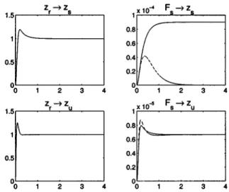
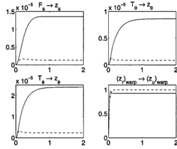
(59) It is interesting to note that in (58) is a scalar matrix due to the fact that is itself scalar (see (30)). This controller gives the dc gains and
as 1.32 10 and 8.39 10 , respectively, compared with 1.36 10 and 8.64 10 using passive control. The step responses using the two controllers are shown in Fig. 13.
B. Roll Control
Referring to Table IV, the roll mode of the full-car corre-sponds to a quarter-car with the following coefficients:
kg, kg, kN/m, kNs/m,
kN/m. The required structure of takes the fol-lowing form after using Table IV, (19), and (51)
(60)
Fig. 14. The warp quarter-car. Given the weighting function
(61) such that the weighted plant has a bandwidth of about 60 rad/s, it is found that the loop shaping controller after model reduction is given by
(62) where is given by (59). (This controller is the same as the diagonal terms in since the weighted plant
is the same as the diagonal elements in the scalar matrix , see (30) and Table I.) This controller gives the steady state gain of as 2.33 10 , compared to the
passive suspension with dc gain , a
similar result to Fig. 6.
C. Warp Control
For the warp quarter-car, we will take a slightly different ap-proach for the design of the active controller. Since the sprung mass cannot be twisted, i.e., it has no warp motion, there is no corresponding role for the active controller to make the “sprung mass” stiffer to the loads. On the other hand, even though the passive road disturbance responses were designed to be rel-atively soft, there is no reason why they should not be even softer in the warp mode. We will therefore abandon the goal of keeping the response to the road warp input invariant under active control. We also note that there is no accelera-tion measurement associated with warp and so there is only one feedback signal available corresponding to the strut deflections: . For this reason there is no block for the warp quarter-car loop in Fig. 12.
Referring to Table IV, the warp quarter-car reduces to the form illustrated in Fig. 14, with and the coefficients
kg, kN/m, kNs/m and
kN/m. The dynamic equation then takes the form, using (13)–(15)
which reduces to, using (10) and (11)
(63) with the correspondences given in Table IV.
We now claim that it is desirable to choose so that
to justify this. If we consider the case where the full-car model
is in equilibrium with , then the (39)–(41)
are equivalent to
(64)
Evidently there is one degree of freedom available in the sus-pension forces, and indeed we can check that
(65) for some constant , completely characterizes that freedom. From the point of view of reducing the amount of “twist” on the vehicle chassis which the suspension forces impose, it would be desirable to achieve a value of in the steady state. The following result shows that the above mentioned condition achieves this property.
Proposition 1: Suppose the (linearized) full-car model
de-fined in Section V-A is in equilibrium with
and arbitrary. Then the following equation holds: (66)
if and only if .
Proof: Using (49) and (53), we notice that the warp
vari-able is a combination of variables at the four wheel-stations
where can be or . Using (46) and
(47) we see that (66) is equivalent to
, which is equivalent to
by (42)–(45), which in turn is equivalent to by (65).
It can be observed that the proposition holds if (66) is replaced by any equation of the form:
with , i.e., the particular ratios chosen in the definition of the warp variable are not critical to the result.
Now let us return to the warp quarter-car represented in (63). If we choose a simple constant controller and ignore temporarily the actuator dynamics, i.e., set , then the choice of achieves a damping ratio of one, a natural fre-quency equal to 50 rad/s (which is lower than the bandwidth of the actuator) and a steady-state gain of 2. As shown by Proposi-tion 1 we would like to achieve the condiProposi-tion (66) in the steady-state, which is equivalent to the dc gain . Setting achieves in (63) a damping ratio of one, a natural frequency equal to 70.71 rad/s (which is lower
Fig. 15. Final controller structure for the full-car model.
Fig. 16. Step responses using active (dashed) and passive (solid) suspensions. than the bandwidth of the actuator) and a steady-state gain of one. In order that the controller is proper, we can choose
(67) The response does not change significantly with this modifica-tion or when the actuator dynamics are included. The step re-sponse with the final controller, with improved warp behavior compared to the passive case, is shown in Fig. 16.
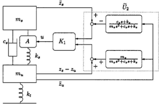
D. The Full-Car Control
As a final step we can redraw Fig. 12 in the form of Fig. 15 where is the full-car model represented by (39)–(45). In Fig. 15 the measurements and control signals are defined as follows:
where and represent the strut deflection and control com-mand signal at each wheel station. The blocks are defined as follows:
where is defined in (48), is defined in (52) and
Fig. 17. Response ofz to a step input of 1 cm atz for AutoSim model using active (dashed) and passive (solid) suspension.
. Note that combines defined in (56) and defined in (60), and the third row in reflects the fact that there is only one measurement available for warp control. The controller is defined as
where , and are given by (58), (62) and (67), re-spectively. Compared with the passive suspension, the benefits of using active controllers is shown in Fig. 16. The responses to “bounce,” “pitch,” and “roll” road inputs are not shown since these are the same in the passive and active cases.
E. Vehicle Dynamics Simulations
In this section we present some simulation results for the controller designed in Section VI-D using the multibody sim-ulation package AutoSim. A nonlinear dynamical model of the simple full-car shown in Fig. 11 was constructed with the sus-pension struts constrained to move perpendicularly to the ve-hicle body. To model a rolling wheel of inertia 1 kg m with tire the magic formula [1] was employed to calculate the acceler-ating and braking forces. The control law given in Section VI-D was implemented together with the actuator structure described in Section V-A.
The model was first tested at zero velocity for various road disturbance inputs and gave similar results, for small displace-ments, to a Matlab simulation of the linearized model. As ex-pected, the bounce, pitch and roll responses were the same in the active and passive cases. Fig. 17 shows the effect of applying a step input to the AutoSim model at the right front wheel in both the passive and active cases. The difference in behavior is due to the “warp” mode being treated differently in the active case, as explained in Section VI-C.
The AutoSim model was then tested under acceleration and braking. For acceleration, a torque was applied at each front wheel with the opposing reaction torques acting on the vehicle body. A similar approach was taken for braking but with the braking torques applied to the front and rear wheels in a 60:40 ratio. Fig. 18 shows the “squat” and “dive” of the model under acceleration and deceleration, with the forward velocity given in Fig. 18(a) and the pitch angle given in Fig. 18(c). The sim-ulation shows that the active suspension significantly improves the squat and dive performance.
Fig. 18. Antidive and antisquat effect in AutoSim model using active suspension (dashed), compared with passive suspension (solid). (a) Forward velocity. (b) Applied torque on front wheels. (c)z . (d) z .
VII. CONCLUDINGREMARKS
This paper has considered the vehicle active suspension design problem with particular regard for the potentially conflicting performance requirements from two disturbance sources: road irregularities and loads applied to the vehicle body. General theorems (Theorems 1, 2) were derived to parameterize all stabilizing controllers which leave some prespecified closed-loop transfer function fixed. This allowed a feedback controller to be designed taking account of only the load disturbance path objective, given that the controller structure ensured that the road disturbance responses remained satisfactory.
The approach was illustrated for the quarter-car model with various different choices of measurements. The required con-trol structures were derived in parametric form. For a half-car model, a parametric control structure was derived for a typ-ical measurement set: verttyp-ical and angular accelerations of the sprung mass and strut deflection measurements. The conditions under which the model structure could be decomposed into two quarter-cars was investigated. For the full-car model, decompo-sition into two half-cars was exploited under a mild symmetry assumption. This enabled the bounce/pitch half-car design to be carried out with the half-car structure previously derived. For the roll/warp half-car a further decomposition into two quarter-cars was assumed. This allowed the warp quarter-car to be treated in a distinct way, which is necessary since the load disturbance path is absent here and it is also reasonable to change (i.e., soften) the road disturbance response from the passive case. A controller was designed and demonstrated on a nonlinear ve-hicle dynamics model and showed the effectiveness of the de-sign for reduced dive and squat under acceleration and braking, improved warp response and invariance of other road distur-bance responses.
A key step in the method described in this paper is the com-putation of the matrix which determines the required con-troller structure. Throughout the paper it was always possible to calculate symbolically using Maple. For more complicated vehicle models this may not be feasible. In such a case a direct numerical approach may be possible. Let us consider the case , i.e., the matrix in (6) is square. (This condition applied throughout this paper and seems quite typical in gen-eral.) Then the following procedure can be taken: 1) partition where is square; 2) find a minimal realiza-tion of ; and 3) find a left coprime factorization
and set (e.g., see [30, Theorem
12.19]. Such an approach was taken in a trailing-arm vehicle model in [23].
APPENDIX
Proof of Lemma 1: can be decomposed in terms of its
Smith form over [21]: , where ,
are unimodular, . Suppose that has
nonzero diagonal elements. Then we can write
(68) (69)
where . We also partition and conformably:
, where ,
, , . We therefore
obtain
where , are full column normal rank
and full row normal rank, respectively.
Proof of Theorem 1: A stabilizing controller in
the form (3) leaves if and only if
. This is equivalent to since (respectively, ) has full column (respec-tively, row) normal rank. We now show that it requires to take the form given in (7). Clearly
(70)
for some . This gives
Next we see that
(71)
for some , which establishes (7).
Conversely, if (7) holds for some and
, then so does (71), from which follows
which again implies .
Proof of Lemma 2:
1) In this case , which
means any element of is also an element of .
Suppose , then for any there
exist some such that . Let
us now choose the first row of to be
(with the one in the th place), and all other rows to be zero, and define to be the first row of the corresponding
. Then , from which we
conclude that where .
2) From 1) we know that if and only if
and for some , . Hence we
have which gives
. Since is full row normal rank, it is equivalent to , which is equivalent to and being unimodular and inverses of each other over .
Proof of Theorem 2:
1) 2) These conditions allow us to choose , ,
, , , , and
. Then (8) follows directly from (3) and (7).
3) Consider and such that all stabilizing
controllers can be parameterized as ,
and ,
, respectively. We can check that
if and only if . From Lemma
2, this means there exits a unimodular matrix such
that .
4) Since , have elements in , it follows from [30, Corollary 5.5] that stabilizes if and only
if , which is
equivalent to
since is right invertible over , which is the necessary and sufficient condition that stabi-lizes . To complete the proof, let
and note that
. Therefore will
take the form of (8), from which the result follows. 5) Any stabilizing controller for which
takes the form of (8). We can then define a
controller for some
such that . It can
also be shown directly that
, which means that stabilizes .
Proof of Corollary 1: Using the parameterization of Theorem 2(2), it follows from (4) that the closed-loop
transfer function remains the same as when
is applied if and only if , which is
equiva-lent to , which results in (9) by using
REFERENCES
[1] E. Bakker, L. Nyborg, and H. B. Pacejka, “Tyre modeling for use in vehicle dynamics studies,” Soc. Automotive Eng. Trans., vol. 96, pp. 190–204, 1987.
[2] D. A. Crolla and A. M. A. Aboul Nour, “Theoretical comparisons of various active suspension systems in terms of performance and power requirements,” in Proc. IMecE Conf. Advanced Suspensions, London, U.K., Oct. 24–25, 1988, paper C420/88, pp. 1–9.
[3] J. C. Dixon, Tyres, Suspension and Handling, 1st ed. Cambridge, U.K.: Cambridge Univ. Press, 1991.
[4] R. J. Dorling, “Integrated Control of Road Vehicle Dynamics,” Ph.D., Cambridge Univ., Cambridge, U.K., 1996.
[5] B. A. Francis, “A course inH control theory,” in Lecture Notes in
Control and Information Sciences. Berlin, Germany: Springer-Verlag, 1987.
[6] K. Hayakawa, K. Matsumoto, M. Yamashita, Y. Suzuki, K. Fujimori, and H. Kimura, “RobustH feedback control of decoupled automobile active suspension systems,” IEEE Trans. Automat. Contr., vol. 44, pp. 392–396, Feb. 1999.
[7] J. K. Hedrick and T. Butsuen, “Invariant properties of automotive sus-pensions,” Proc. Inst. Mech. Eng. J. Automobile Eng., pt. D, vol. 204, pp. 21–27, 1990.
[8] D. Hrovat and M. Hubbard, “Optimal vehicle suspensions minimizing RMS rattlespace, sprung-mass acceleration and jerk,” Trans. Amer. Soc.
Mech. Eng., vol. 103, pp. 228–236, 1981.
[9] D. Hrovat, “A class of active LQG optimal actuators,” Automatica, vol. 18, pp. 117–119, 1982.
[10] D. Karnopp, “Theoretical limitations in active suspension,” Veh. Syst.
Dyn., vol. 15, pp. 41–54, 1986.
[11] D. C. McFarlane and K. Glover, “Robust control design using normal-ized coprime factor plant descriptions,” in Lecture Notes in Control and
Information Sciences. Berlin, Germany: Springer-Verlag, 1987. [12] K. M. Malek and J. K. Hedrick, “Decoupled active suspension design
for improved automotive ride quality/handling performance,” Veh. Syst.
Dyn., vol. 15, supplement, pp. 383–398, 1986.
[13] P. E. Mercier, “Vehicle suspensions—A theory and analysis that accord with experiment,” Automobile Eng., vol. 32, pp. 405–410, 1942. [14] K. Park and J. J. Bongiorno Jr, “Wiener-Hopf design of
servo-regu-lator-type multivariable control systems including feedforward compen-sation,” Int. J. Contr., vol. 52, no. 5, pp. 1189–1216, 1990.
[15] R. Pitcher, H. Hillel, and C. M. Curtis, “Hydraulic suspensions with par-ticular reference to public service vehicles,” in Proc. Public Service Veh. Conf., 1977.
[16] R. S. Sharp and S. A. Hassan, “On the performance capabilities of active automobile suspension systems of limited bandwidth,” Veh. Syst. Dyn., vol. 16, pp. 213–225, 1987.
[17] , “The relative performance capabilities of passive, active and semi-active car suspension systems,” Proc. Inst. Mech. Eng., vol. 200, pp. 219–228, 1986.
[18] M. C. Smith, “Achievable dynamic response for automotive active sus-pension,” Veh. Syst. Dyn., vol. 24, pp. 1–33, 1995.
[19] M. C. Smith and G. W. Walker, “Performance limitations and constraints for active and passive suspension: A mechanical multi-port approach,”
Veh. Syst. Dyn., vol. 33, pp. 137–168, 2000.
[20] A. G. Thompson, “Design of active suspensions,” Proc. Inst. Mech.
Eng., vol. 185, pp. 553–563, 1970–71.
[21] M. Vidyasagar, Control System Synthesis: A Factorization
Ap-proach. Cambridge, MA: MIT Press, 1985.
[22] G. W. Walker, “Constraints Upon the Achievable Performance of Ve-hicle Suspension Systems,” Ph.D. dissertation, Cambridge Univ., Cam-bridge, U.K., 1997.
[23] F.-C. Wang and M. C. Smith, “Active and passive suspension control for vehicle dive and squat,” in Automotive Control Workshop, Lund, Sweden, May 18–19, 2001. To appear in “Nonlinear and Hybrid Systems in Automotove Control,” R. Johansson and A Rantzer, Eds. London, U.K.: Springer-Verlag.
[24] R. A. Williams and A. Best, “Control of a low frequency active suspen-sion,” Control ’94, vol. 1, no. 389, pp. 338–343.
[25] R. A. Williams, A. Best, and I. L. Crawford, “Refined low frequency active suspension,” in Proc. Int. Conf. Vehicle Ride Handling, Birm-ingham, U.K., Nov. 1993, C466/028, pp. 285–300.
[26] P. G. Wright and D. A. Williams, “The application of active suspension to high performance road vehicles,” in Proc. IMecE Conf.
Microproces-sors Fluid Power Eng., London, U.K., 1984, paper C239/84, pp. 23–28.
[27] , “The case for an irreversible active suspension system,” SAE
Trans., J. Passenger Cars, pp. 83–90, 1989.
[28] D. C. Youla, H. A. Jabr, and J. J. Bongiorno Jr, “Modern Wiener-Hopf design of optimal controllers—Part II: The multivariable case,” IEEE
Trans. Automat. Contr., vol. AC-21, pp. 319–338, 1976.
[29] D. C. Youla and J. J. Bongiorno Jr, “A feedback theory of two-degree-of-freedom optimal Wiener-Hopf design,” IEEE Trans. Automat. Contr., vol. AC-30, pp. 652–665, 1985.
[30] K. Zhou, J. C. Doyle, and K. Glover, Robust and Optimal
Con-trol. Upper Saddle River, NJ: Prentice-Hall, 1996.
Malcolm C. Smith (M’90–SM’00–F’02) received
the B.A. degree in mathematics in 1978, the M.Phil. degree in control engineering and operational research in 1979, and the Ph.D. degree in control engineering in 1982 from Cambridge University, Cambridge, U.K.
He was a Research Fellow at the German Aerospace Center, Oberpfaffenhofen, Germany, a Visiting Assistant Professor and Research Fellow with the Department of Electrical Engineering, McGill University, Montreal, QC, Canada, and an Assistant Professor with the Department of Electrical Engineering, The Ohio State University, Columbus. In 1990, he joined the Engineering Department at the University of Cambridge, U.K., as a Lecturer and subsequently Reader in 1997. His research interests include robust control, nonlinear systems, and automotive applications.
Dr. Smith is a co-recipient with Dr. Tryphon T. Georgiou of the 1992 and 1999 George Axelby Best Paper Awards in the IEEE TRANSACTIONS ONAUTOMATIC CONTROL.
Fu-Cheng Wang (S’00) was born in Taipei, Taiwan,
R.O.C., in 1968. He received the B.S. and M.S. degrees in mechanical engineering from National Taiwan University, Taipei, Taiwan, R.O.C., in 1990 and 1992, respectively, and the Ph.D. degree in control engineering from Cambridge University, Cambridge, U.K., in 2002.
Since 2002, he has been a Research Associate in the Control Group of the Engineering Department, Cambridge University. His research interests include H control, vehicle active/passive suspension con-trol, loop-shaping, and fuzzy systems.