9 1994 Kluwer Academic Publishers. Printed in the Netherlands.
Identification Environment and Robust
Forecasting for Nonlinear Time Series
B E R L I N WU
Department of Mathematical Sciences, National Chengchi University, Taiwan (Received: June 1992)
Abslract. In this paper, the methods of time series for nonlinearity are briefly surveyed, with particular attention paid to a new test design based on a neural network specification. The proposed integrated expert system contains two main components: an identification environment and a robust forecasting design. The identification environment can be viewed as a integrated dynamic design in which cognitive capabilities arise as a direct consequence of their self-organizational properties. The integrated framework used for discussing the similarities and differences in the nonlinear time series behavior is presented. Moreover, its performance in prediction proves to be superior than the former work. For the investigation of robust forecasting, we perform a simulation study to demonstrate the applicability and the forecasting performance.
Key words, nonlinear time series, bilinear, Lagrange multiplier test, neural network, forecasting, robust.
1. I n t r o d u c t i o n
T h e analysis in time series models has b e e n concerned with processes which are stationary. Tests for unit roots in time series data have b e e n the subject of a t t e n t i o n in econometrics as well as with statisticians in the last two decades. M u c h of the research has concentrated on the distribution theory that is necessary to d e v e l o p these tests and the analysis of the p o w e r of various tests u n d e r different alternative hypotheses. H o w e v e r , in a m a j o r i t y of economics applica- tions the need of a nonlinear tes~t is a priori rather than unit roots test for nonstationarity. As the papers by T s a y (1991), G r a n g e r ( 1 9 9 t ) , and G o o i j e r and K u m a r (1992) indicate, the interest in applying nonlinear time series models has considerably increased recently. T h e r e also seems to be strong belief a m o n g economists that relationships b e t w e e n economic variables are nonlinear; pro- duction m o d e l being an example. Specifically, given p a r a m e t r i c relationship, such as the C o b b - D o u g l a s or C E S production models, standard econometrics tech- niques p r o v i d e ways of estimation of the p a r a m e t e r s as well as its asymptotic p r o p e r t i e s ; see G r a n g e r (1991).
T h e results o b t a i n e d thus far did not provide efficient rules in testing w h e t h e r or not the correct nonlinear specification has been achieved or w h e t h e r there still r e m a i n s s o m e neglected nonlinearity in the estimated relationship. In o t h e r words, w h e n the underlying models are not correctly specified, very few statistical
38 BERLIN WU tests can provide a well-designed procedure for model identification and parame- ters estimation. Since uncertainties usually exist about the correct underlying statistical models, the dynamic form, lag structure and the stochastic assumptions have a heavy impact on the power of the tests and the forecasting performance. Therefore, to propose a robust procedure for identifying nonlinear time series, as
well as accurate forecasting, is what we are most concerned about.
The problems of identifying nonlinear time series, that we propose, can be
divided into two groups: model based and model free systems. Up to now, most of the former work has relied on diagnostics such as Lagrange Multiplier test, Bispectrum test, Likelihood ratio-based tests and arranged autoregression test... ; etc. Expository papers in L M testing are Luukkonen et al. (1988) for testing
S E T A R / T A R type nonlinearity and Saikonen and Luukkonen (1988) and Guegan and Pham (1992) for testing simple bilinear type nonlinearity. The L M
test against the A R C H model can be found in Weiss (1986) and Saikonen and Luukkonen (1991). Hinich (1982) used the Bispectrum test to identify the bilinear
models. Chan and Tong (1986) used Likelihood ratio-based tests for SETAR
models. Tsay (1989), (1991) presented the arranged autoregression method for
testing T A R models. Unfortunately, these available tests are based on a particular class of nonlinear time series models. None of the above tests has dominated the others with reasonable power. For instance, the L M test is
designed to reveal specific types of nonlinearity. The test may also have some power against incorrect alternatives. There may, at the same time, exist alter-
native nonlinear models against which an L M test is not powerful. Hence,
rejecting ~0 on the basis of this test does not allow very strong conclusions about the type of possible nonlinearity.
On the other hand, an interesting research topic for nonlinear systems has arised in the study of neural networks. This is, recently, an area of considerable
applications due to its potential for providing insights into the kind of highly parallel computation that is carried out by physiological nervous systems. Recently, many computer-based analytical models have been developed and the neural networks technologies have been extensively studied by many researchers, e.g., Grossberg (1988) and his colleagues provided much of the theoretical foundation for these systems; Lapedes and Farber (1988) at Los Alamos National Laboratory have used backpropagation networks for making prediction and
system modeling; Ramey (1989) and Kosko (1991) suggest various applications, including fuzzy theory, for neural networks. Detailed expositions of the approxi- mation and network learning theory can be found in the book of White (1992), which also provides a fundamental link between network learning and modern mathematical statistics. Recently, Chatfield (1993) suggests that it is possible that neural nets will outperform standard forecasting procedures w h e n a fair com- parison is made, at least for certain types of situations.
The use for neural networks in forecasting is a new approach for the time series analysis and is developed in Section 4. Methodologically, the outlined strategy
requires the analysis of the following procedures: (a) constructing the adequate neural system; (b) data pre-processing procedure; (c) network initiation; (d) learning and training; (e) forecasting.
The goal o f this paper is to propose a network system which integrates nonlinear testing and neural network identifier techniques and performs a robust forecasting. Neural networks, with its testing processes, can be viewed as an integrated dynamic design in which cognitive capabilities arise as a direct consequence of their self-organizational properties. The robust properties for forecasting performance are discussed by comparing them with other model-based procedures.
2. Integrated Identification Environments
Since a lot of economic time series cannot be linearized, we will consider an alternative technique for model structure and identification. In this section we will give an integrated nonlinear testing environment. Genetic operators allow the system to learn from experience and modify its behavior in reaction to stimuli coming from an external environment which is (possibly) evolving in time.
The principle components of an identifying system are: 9 a finite set of rules ~ = ( ~ 1 , . . - ,~1} (the identifier);
9 a set of detectors, which provide the system with information about the state of external environment;
9 a set of erectors, which send the outputs of the computation to the external environment;
9 a message list, where the detectors post their message, and where the erectors pick their activation signals.
An identifier I i E 3- is a tuple (/~1, Ii2; Ag, S~), where Igj denote the conditions that have to be satisfied for I i to become active, A~ denote the type of message that will be produced by I i when it is activated, i.e., Ai is a template that may use some information contained in the message that match the I~j's to produce the new message, s~ is a real number (the strength) which quantifies how good the identifier is, i.e., how useful it is, in a sense which will be made clear when we describe the mechanism of the system.
Identification of time series Xlt and
S2t
c a n be based on the threshold values of each data for the category membership. For each data D~ the membership in the category can be the following calculation:1, then category I i
I f sign(output Di) = O, then category I z (2.1) Expression (2.1) describes the decision function of the identifier designed by
40 I n p u t o
Identificationll
Environment
,Distance
[]Category
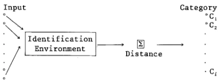
~ I ~ 2 9 C~Fig. 1. Integrated identification environment.
B E R L I N W U
inspection of the set that needs to be classified. The dynamic process is shown in Figure 1.
Though the design looks simple, its operation becomes far more involved and intriguing when requirements for membership in categories become complicated.
2.1. I D E N T I F Y I N G P R O C E D U R E S
The identifier system performs a sequence of test procedures which include (i) pattern classification of date set (ii) order selection and (iii) parameters estima- tion. And consist the following steps:
(1) Time series acquisition: ACF, PACF, CCF, cumulant, bispectrum, polyspec- trum. etc.
(2) If time series data set passed the linearity and stationarity test: LM test
Bispectrum test, Likelihood ratio-based tests
orarranged autoregression test,
etc. Then go to final step (7); otherwise go to step (3).
(3) Diagnose on correlation dimension, Kolmogorov entropy, and Lyapunov exponents, Lagrange multiplier, etc.
(4) All identifiers with satisfied conditions enter a competition to generate messages for the new message list. The competition consists, in each identifier, of making a bid, and the winning identifiers become
active
and post their messages9(5) If messages indicate a special nonlinear type, complete this model construc- tion, then go to step (7); otherwise go to step (6).
(6) The effects check the new message list and produce new actions (the output of the identifier system) according the messages they find. It is possible that no action takes place9 An extended identification system is considered.
(7) Output the result.
It is clear that the identifier systems are inherently parallel systems. In fact there is an obvious correspondence between the message-passing scheme used by classifiers to communicate and communications between units in a parallel machine. In the above processes, the rules that responded
correctly
to the stimuli of the environment increase their strength, while those that participated in computations which led to wrong answers are weakened. These new identifiersreplace the weak ones in an attempt to improve the overall performance of the system. This genetic is essentially random; actually, the selection of the loci for the cross-over and the mutation operations is made following a flat probability distribution, while the prospective parents are usually chosen according to a probability distribution. In practice other genetic operations are introduced to improve the learning performance system.
Another important feature is that one can provide a set of pre-defined rules to help the system in the search for an adequate behavior. In other words, partial information may be provided to shorten the learning stage. This differs from the case of neural networks, where the rules followed by the system are distributed in the connection strengths, and it is hard to give a meaning to the connections in terms of rules discovered by the system.
In an identifier system it may happen that different messages generate equal or different messages through the same identifiers in the same time point. In other words, the same identifier can connect different couples of cells and many copies of its are generally brought into play on each major cycle. Cells without connections can be conceived of as being linked to the remaining cells by virtual connections with strength set to zero. Also notice that two distinct nodes n i , nj may have several connections, corresponding to different identifiers 9- such t h a t
= n j .
3. Neural networks and Model-Free Forecasting
Bilinear time series comprise the simplest class of nonlinear time series. In its most general form a bilinear time series {X~} with discrete parameter is defined by
q
2 s
X t - ~,, a j X t _ j = e, + ~ Oje,_j + b i j X t _ i e , _ j ,
j = l j = l i = 1 j = 1
(3.1)
where e t is a strict white noise process with finite variance
0"26.
This model is called B L ( p , q, m, n).In some practical applications, numerous bilinear models have been studied in physics, seismology, engineering, ecology, etc. These include, e.g., nuclear fission reactors (Mohler, 1963) and biomedical processes (Mohler and Ruberti (1978), and Marchuk (1983)). Heating, ventilating, air conditioning systems, solar panels, and storage tanks, may be similarly modeled by the bilinear state space model. Such analyses result in significant energy saving over the traditional linear optimal control approach. Bilinear models are coupled together so that the total model is more highly nonlinear. Such model coupling may be linear or nonlinear, depending on the particular process under investigation.
Granger and Anderson (1978) pointed out that some simple bilinear series have zero second order autocorrelation and might be mistaken as white noise or an
42 BERLIN WU
A R M A model with higher order. Suba Rao and Gabr (1984) have proposed a method about model identification and parameters estimation of B L ( p , O, m, n), but it takes a lot of computations and iterations. Wu and Shih (1992) suggest a more efficient process than Subba Rao and Gabr's method for simple bilinear models. However, for general bilinear time series, there is no consistent and efficient method for solving the identification problem so far. Not even for the forecasting of bilinear models.
The neural networks approach, as an area of considerable recent interest due to its potential for providing insights into the kind of highly parallel computation, has found a general approximation for any unknown functions, providing that enough input and output data are given for training the neural networks. The ability to estimate, test, model, forecast and control the underlying system provides great incentive.
Since neural networks are general approxirnators for the unknown functions, no assumptions are made for the data. That is, no prior models are built for the unknown functions. This characteristic is quite different from that of A R M A models. In A R M A (or vector ARMA) models, it is assumed that the time series should be linear and stationary. While the special capability of neural networks makes themselves a robust analysis tool for various patterns of time series.
3.1. PERCEPTRONS
Neural networks have many variations. Recent developments in the neural network theory (see Cybento (1989), Funahashi (1989), Hecht-Nielsen (1989), Amari (1990), Kolen and Goel (1991), and Kosko (1992) show that multilayer feedforward neural networks with one hidden layer of neurons can be used to approximate any Borel-measurable function to any desired accuracy. The concept implies that if the nonlinear law governs the system, then even if the dynamic behavior is chaotic, the future may to some extent be predicted from the behavior of past values that are similar to those of the present.
The outputs of neurons in one layer are transmitted to neurons in next layer through links. The interconnection weights between neurons in two adjacent layers l and l + 1 are written by the weight matrix W~ = (wl,ij). The ith row of W 1 corresponds to the input weight vector for the ith neuron in layer 1 = 1. The input set of the network contains all the neurons in the first layer and the output set of the network, all the neurons in the 1st layer. Neural networks act as a function, mapping the input space R '~ to the output space R". The net input to a neuron i in layer l is
1
I1, i = ~ Wl.ijO1, j . (3.2)
j = l
0 1 , i :
g(Ii,i) ,
(3.3)where g is traditionally the sigmoid function but can be any nonlinear differenti- able function. For a sigmoid activation function, we have
1
(3.4)
O l ' i ~-- i "~-
e -~(II,i+~
'where A, called
the slope of the shape,
is used to control the steepness of the function. The effect of the threshold value 01, i is to shift the function along the horizontal axis.Then, each neuron in layer 1 + 1 performs a summing and applies a threshold function of the following form:
O1+1'i = g(]~l=
wl'i]Ol' ])'
(3.5)where O~+x, i is the output of the ith neurons in the l + 1 layer.
3.2. NEUROCOMPUTING FOR THE LEAST MEAN SQUARE LEARNING SYSTEM We now present a device for the identification of certain sets of bilinear time series. The network weights are to be chosen so that a preselected set of binary N-vectors are obtained by squashing equilibrium solutions. These binary vectors will be called memory traces stored by the network. Any initial condition for the network state vector may be used to probe the network, and the resulting steady-state network output vector is called the
evoked response.
In the first place, we determine the error function as e 1 = Or-01 = output v e c t o r - estimated output vector. The parameter adaptation of the network is done by adjusting the interconnection weight wl,,-j and the thresholds
01, i
toward the direction of minimizing the mean squared error. The total system error is1
: = O l , i ) 9
(3.6)
1
Using the steepest decent technique, we then update the linkweight as follows:
new old A old
W l , i j -~ W l , i j -~- / ~ W l , i j
old ~_ AVw~ 1
: W l , i j (3.7)
Clearly, the direction of the maximum decreasing is given by --~Tw~ 1 = - - ( ~ 1 /
0w;j). To prove that ~1 is differentiable, interests readers may refer to Hecht- Bielsen (1988). We achieve convergence toward the improved values for the
44 BERLIN WU weights and thresholds by taking incremental changes Awt, o proportional to
--O~/3wl,ij,
that is,Awl, q = - A Owl,i---i,
(3.8)where A, called learning rate, is used to control the convergent speed of the learning process. A large A would make the learning speed faster, but is more likely to cause the system to become unstable.
Using the chainrule, the partial derivative
O~i/Ow 1 ij
becomes3 I i , i 3 W l , i j - 311, i 3 W l , i j _ Wl,i. iO1, j
= 011, i 0 1 , j , (3.9)
Let 31, i =
-(3~1/011,i).
Combining with (3.8) and (3.9) givesm W l , i j = l ~ l , i O 1 , j . (3.10)
If the layer l is not the output layer, then
O~ 1 Ool,i
~ 1 , i - 0 ~ 1 , i
011, ~
O_
[ 1 +
j) ]g
(Ii,i)
- - 0Ol,ik 2 ~ (O1' j - ()1, 2 t
= (Ol, i - ~ l , i ) g ' ( I i , i ) .
(3.11)
Thus, we calculate the change of the weight between neuron i and every neuron k (including the pseudo) in layer l, and modify the weights:
new old ~ old Wl,i] = W l , i j + OWl,ij
old old 0
= W l , i j + A ~ 1,i O1 9 (3.12)
3.3. T H E P R A C T I C A L A P P L I C A T I O N O F B A C K - P R O P A G A T I O N
As with the original least mean square training procedure, the learning rate parameter A plays an important role in the practical application of Back-propaga- tion. For a given network and an infinitesimal earning rate, the weights that yield the minimum error can be found. However, they may not be found in our lifetime. While it is possible to get excellent fits to training samples, the application of back-propagation is fraught with difficulties for the forecasting performance on test samples. Unlike most other learning systems that have been
previously discussed, there are far more choices to be made in applying this gradient decent method. Even the slightest variation can make the difference between good and bad performance. While we will consider many of these variations, there is no universal answer to what is best. The major route for getting the best results is through repeated experimentation with varying ex- perimental conditions. Steps for building neural networks are listed below.
(a) Deciding the number o f systems layers and nodes. Cybento (1989) proved
neural networks with one hidden layer are sufficient for a function approximator. T H E O R E M 3.1 (Backpropagation Approximation Theorem) Let g be a bounded, measurable sigmoidal function. Then the finite sums o f the form
N
G(x) = ~ .~j(1, 2~ gtt-"~'(~ J 1),vj.~ - Oj) , (3.13) y=l
are dense in C([0, 1]m). In other words, given any e > 0 and f E C([0, 1]m), there exists a three-layer Backpropagation neural network that can approximate f within e mean squared error accuracy.
This theorem resembles the Weierstrass approximation theorem: every continu-
ous function on a compact interval is the limit of a uniformly convergent sequence of polynomials. It is important to note that although this theorem shows that three layers are enough, in processing real-world data it is often designed to have four or more layers. This is because for many problems an approximation with three layers would require an impractical large number of hidden units. The problem of hidden neuron size choice is under intensive study, for example, see Kosko (1992) and Wu, Liou and Chen (1992). The exact analysis is rather difficult because of the complexity of the network mapping and due to the non-determinis- tic nature of many successfully completed training procedures.
(b) Random initial state. Unlike most other learning system, the neural network
begins in a random state. The initial weight of each link is randomly assigned between - 1 and 1. The reason for assigning weights within this interval is that the activation function of each hidden unit is a sigmoid function. The sigmoid function has the most steep slope near zero. To assign weights near zero will have most significant learning speed.
(c) Normalization o f data. Since the input domain of the neural network
activation functions are limited, the data are usually normalized to an appropriate interval. The scale/location transformation are performed for the input data and are usually to the interval [0, 1]. The output value of sigmoid function falls into the same interval. An inverse transformed will be taken to get the estimate values of the original form.
46
B E R L I N W Umatrix W to achieve desired result is called learning. The selection of a learning rate is of curtailed importance in finding true global minimum of the error distance. Too small of a learning rate will make agonizingly slow progress. Too large of a learning rate will proceed much faster, but may simply produce oscillations between relatively poor solutions. Both of these conditions are generally detectable through experimentation after a number of training epochs. Empirical evidence support the notion that the use of momentum conception can be helpful in speeding convergence as avoiding local minimum (see Weiss and Kulilowski, 1990). Momentum towards convergence is maintained by making nonradical revisions to the weights.
(e) Stopping rules. We pre-assign an accuracy measure, and if the error reaches to the assigned preassigned value the iterative procedure will halt. In practice, for an arbitrary neural net, the convergent rate may be very slow.
( f ) Model-free forecasting. After a neural networks is properly built, we use it to predict future value by inputting the present data without knowing its specific model.
4. Performance of Forecasting on Simulated Study 4.1. A N I L L U S T R A T E D E X A M P L E
Our study is focused on simple bilinear time series because they are frequently encountered in practice, and because they are widely used in the literature.
f X t + l set 4.1:1xt+1 [.Xt+ l f Xt+l set 4.2:~xt+1 LXt + 1 f X t + l set 4.3:ixt+1 L X t + I f X t + l set 4.4:Ixt+1 I. Xt+l
I
X t + l set 4.5: 9 Xt+l l X t + l = 0 . 2 x t e t + Et+ 1 = O . 5 x t e t q- 8t+ 1 ; = 0 . 8 X t E t -.[- et+ 1 = 0 . 2 X t _ l e t + s t + 1 = 0 . 5 X t _ l e t .-[- et+ 1 ; = 0 " 8 X t - l E t '~ Et+l -= 0 . 2 X t E t _ 1 -t- Et+ 1 = 0 . 5 X t E t _ 1 -.[- et+ 1 "~ =- 0 . 8 X t E t _ 1 -1- et + 1 = 0 . 2 X t + 0.2Xte t + et+ 1 0 . 5 x t -[- 0 . 5 x t e t --}- Bt+ 1 ; 0 . 8 X t + 0 . 8 X t 8 t + St+ 1 =0.2x,
+ 0 . 2 x t e t - 0 . 2 X t _ l e t _ 1 + el+ 1 0 . 5 x t + 0 . 5 X t E t -- 0 . 5 X t _ i E t _ 1 -.[- Et+ 1 ; 0 . 8 X t + 0 . 8 X t E t -- 0 . 8 X t _ l S t _ l + Et+ 1t = l , . . . , n .
Sample sizes 500 were obtained as follows. The normally distributed innova- tions e t --N(0, 1), were generated by using M i n i t a b 8 . 2 s o f t w a r e on a 486-PC computer. The last 8 observations were kept for the comparison of forecasting performance. Let the initial value x ~ = 1.0, the following data sets are realization of bilinear models (i) to (v) and draw in Figure 2.
Neural networks approaches f o r bilinear time series
According to the procedure stated at section 3, we design a neural networks as follows.
9 Inputs & Outputs. Because the decision of the layers and nodes numbers
relies on proper training data, there are no strict answer for it. It is because an approximator with three layers would require an impractical large number of hidden units. Another question of choosing the hidden neurons' size is under intensive study (Kosko (1992) and Wu, Liou and Chen (1992)). The rules for getting more optimal results are to repeat our experimentation with varying experimental conditions. To sum up, the networks must efficiently integrate the largest possible number of relevant factors. For instance, the AR(p) model used for this type of problem suggests p-neurons the number of input. One output is designed for the neural system to give the predictions. We should note that p is just a good suggestion.
9 Data Standardization Transformation. We standardized the data by setting
o l d X i n e w ~ -
Xi m a x { x t } -- m i n ( x t } 9
This transformation serves as a dynamic range limiter.
9 The n u m b e r o f hidden layers and hidden neurons. The hidden layers represent the equivalent of feature space. The difficulty resides in determining the number of hidden layers, for each one the number of neurons and propaga- tion law. According to our experiences, one hidden layer is enough for training linear time series while two hidden layers are appropriate for training a nonlinear time series. Each hidden layer contains about 40 neurons, and generates 1600 links between the hidden layer. Larger networks are more capable. But the computer memory is limited.
9 N e t w o r k s initialization. We train the neural network more than 20,000 times, until the error level is accepted, and the system is approximately close. We set the network initial conditions as:
48 BERLIN WU 4 9
2~
0 -2 t -40 200 4(30 Xt+ 1 = 0.2XtE: t + e t + t (4.1.1) 200 4o
-10 -200 260 460 X t + l ~--- O.~{Xts + g:t+l(4.1.3)
-50 2O0
400 Xt+ 1 = 0.SXt.lCt + Ct+ t (4.2.2) 600 ;00 600 10 5 0 -50 4 2 0 -2 - 4 20 ' 400 2OO xt+ l = 0.Sxtc t + ct+ 1 (4.1.2) '4{)0
200 Xt+ 1 = 0 . 2 X t . l c t q'- Ct+ 1 (4.2.1) o 0 -10 200 400 Xt+ 1 = 0.~O~t.lc I + c t + 1 (4.2.3) 600 600 600 4 2 0 -2-%
1 260 460 Xt+ 1 = 0.2xtctq + ct+l (4.3.1) Fig. 2. 10 o600
-50
200
460
Xt+ I -~ 0 . S x ~ l . l + Ct+ 1 (4.3.2) Realizations of bilinear models (4.1) to (4.5).10 0 -10 -200 260 400 600 150 X t + l = O'SxtCt-I "~ Ct+l (4.3.3) 100 50 0 -50 J 200 4()0 Xt+ ~ = 0.Sx t + 0.5xtc ~ + ct+ 1 (4.4.2) 600 4 40 X t + l 600 = 0 . 2 X t -1"- 0 . 2 X t ~ t - 0 . 2 X t . l C t . 1 q'- Ct+ 1 (4.5. t) 40 4r zt ol -2! -40 260 460 30 xt+ l = 0.2x t + 0.2xtc t + ct+ l (4.4, t) 600 20 10 0 -100 Xt+l 20 ' 6 200 4 0 = 0.8x t + 0.Sxtc t + ct+ t (4.4.3) 600 ! i 200 400 600 Xt+ l ~--- 0 . S x t "[- O , 5 x t c t - 0 . 5 X l . l e t _ l n t- Ct+ I (4.5.2) 0 -20 -400 260 460 600 xt+1 = 0.8x t + 0.Sx~q - 0.8 xt4et.1 + ct+ 1 (4.5.3) Fig. 2. (continued)
50 BERLIN WU
Output range: [0, i]
Initial (random) weight range: [-0.I, 0.1] The slope of sigmoid function: 0.5
Learning rule : Delta rule.
9 Training and learning.
The time of training is dependent upon the characteris-tics of neural networks. While more training time will facilitate the networks r e m e m b e r the pattern of function well, it may ignore the slight local variant in the pattern of the system. On the other hand, less training times correlates to a m o r e sensitive network to the local variance and may get an absurd global pattern for the system.
Stopping rules
Two techniques are presented to determine when to stop:
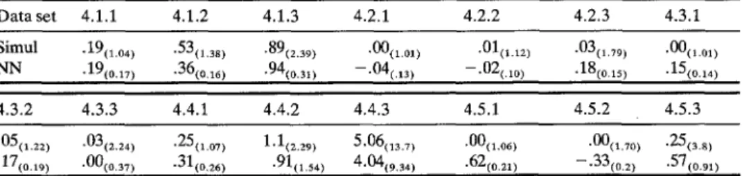
(i) Limit the n u m b e r of epochs: training ceases after a fixed u p p e r limit on the n u m b e r of training epochs. For example, when the training e r r o r yields a pre-assigned value 0.01 or the training epochs are m o r e than 20,000, the training p r o c e d u r e will cease, and the link weights would be used as the final solution. (ii) M e a s u r e d progress criterion: the error can be sampled and averaged over a fixed n u m b e r of epochs, e.g., every 100 epochs of training. If the average e r r o r distance for the most recent 100 epochs is not better than that for previous 100, one might conclude that no progress is begin made, and training should halt. T a b l e 1 shows the mean and variance for the simulated data and the fitted values calculated by designed neural networks.
N o t e that the n u m b e r of input nodes as well as the n u m b e r of the nodes each hidden layer are chosen by
experiments.
T h e r e are numerous combination m e t h o d s in constructing a networks to get a robust fitted for the simulated data. In Table 2, we compare the MSE (mean of square errors) for the neural networks with t h e best fitted A R M A models, which we find are all A R ( 1 ) models according to the Box-Jenkins proceduresandAIC, SBC
criterion. A n interesting and striking result from Table 2 is that the best linear A R M A models fit theTable 1. Comparison of the mean and variance given in the bracket for the realization data with the neural networks approach
Data set 4.1.1 4.1.2 4.1.3 4.2.1 4.2.2 4.2.3 4.3.1 Simul
.19(1.o4)
.53(1,38)
.89(2.39)
.00(1.01)
.01(1.12)
.03(1.79)
,00(1.01)
NN .19(o.17) .36(o16 ) .94(o.31) -.04(.13 ) -.02(.lo ) .18(o.15).15(o.14)
4.3.2 4.3.3 4.4.1 4.4.2 4.4.3 4.5.1 4.5.2 4.5.3
"05(1.22)
"03(2.24)
"25(107)
1"1(2.29)
5'06(13.7)
"00(1.06)
"00(1.70) "25(3.8)
-17(o.19) .00(0.37)-31(o.26)
.91(1.54)
4.04(9.34)
-62(o.21) -.33(o~2) .57(o.91)Table 2. Comparison of MSE for best fitted A R M A models with the neural networks approach Data set 4.1.1 4.1.2 4.1.3 4.2.1 4.2.2 4.2.3 4.3.1 4.3.2 4.3.3 AR(1 ) 1.08 1.85 5.58 1.03 1.24 3.20 1.03 1.44 5,02 NN 0.74 0.56 11.99 0.89 0.61 4.36 0.91 0.53 13,08 Advantage NN NN A R NN NN A R NN NN A R Data set 4.4.1 4.4.2 4.4.3 4.5.1 4.5.2 4.5.3 AR(I~ 1.09 2.77 119.8 1.11 2.76 14.15 NN 0.77 2.65 133.1 0.98 2.27 36.11 Advantage NN NN A R NN NN A R
Table 3. Sum of square error for 8-steps forecasting
D a t a s e t 4.1.1 4.1.2 4.1.3 4.2.1 4.2.2 4.2.3 4.3.1 4.3.2 4.3.3 AR(~ 5.92 3.30 81.55 7.37 4.81 43.14 7.38 4.81 102.9 NN 4.96 2.49 95.92 6.'16 3.93 34.85 5.34 3.21 104.6 Advantage NN NN A R NN NN NN NN NN A R Data set 4.4.1 4.4.2 4.4.3 4.5.1 4.5.2 4.5.3 AR(~) 5.53 10,48 8145 4.70 15.06 212.7 NN 5.05 8,25 3328 3.82 18.21 268.9 Advantage NN NN NN NN . A R A R
bilinear samples from (4.1.3), (4.2.3), (4.3.3), (4.4.3) and (4.5.3), whose coefficients of the bilinear term are high, better than the non-linear neural networks.
Forecasting performance
In Table 3, we c o m p a r e the sum of square error for 8-steps forecasting for the best fitted
A R M A
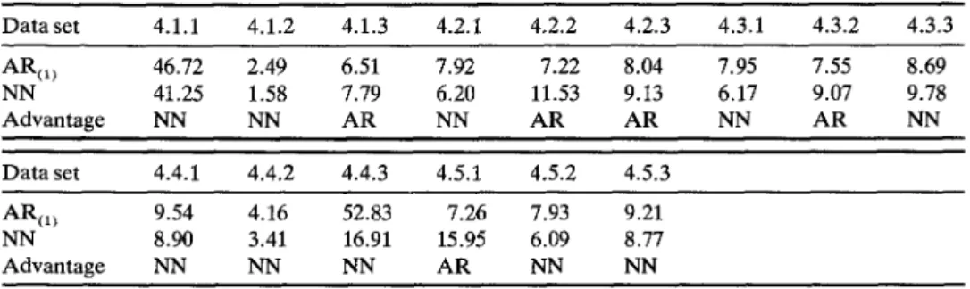
model and the selected neural network. Table 4 compares the sum of absolute percent error for 8-steps forecasting errors.It is shown that the performance of the NN
model
take the advantage to A R as a rate about 2:1. Still we must mention that the neural networks in this research is only abetter
network, the best network structure may be unknown.Table 4. Sum of absolute percent error for 8-steps forecasting
Data set 4.1.1 4.1.2 4.1.3 4.2.1 4.2.2 4.2.3 4.3.1 4.3.2 4.3.3 AR(I ~ 46.72 2.49 6.51 7.92 7.22 8.04 7.95 7.55 8.69 NN 41.25 1.58 7.79 6.20 11.53 9.13 6.17 9.07 9.78 Advantage NN NN A R NN A R A R NN A R NN Data set 4.4.1 4.4.2 4.4.3 4.5.1 4.5.2 4.5.3 AR(I~ 9.54 4.16 52.83 7.26 7.93 9.21 NN 8.90 3.41 16.91 15.95 6.09 8.77 Advantage NN NN NN A R NN NN
52 BERLIN WU
5. Conclusions and Further Research
Two methodologies have been presented in this paper for the identification and forecasting of the nonlinear time series. Having outlined the main features of the identifier system, we can concentrate on its most remarkable properties as compared with traditional test criteria. Our aims are to clarify the degree of similarity between the two classes of systems, and to compare their learning strategies.
The result gained in this research has shown practical applications when the underlying model for the observations are uncertain. The advantage of the neural networks proposed in this article is that it provides a methodology for model-free approximation, i.e., the weighted matrix estimation is independent of any model. It liberates us from the modeling-based selection procedure with no assumptions of the sample data being made.
There remains many problems to be improved, such as:
(i) Problems related to identification: (a) there is a need to develop a procedure for identification for the case of interacting noise; (b) the convergence of the algorithm for combined state and parameters estimation needs to be proved; (c) a solution needed to the power problem based on test statistics in section 2. (ii) Problems relating to network forecasting: (a) Can a particular network be treated as a specific nonlinear design?; (b) In what way does the intial conditions affect the properties of network system?; Does the system become less (or more) sensitive to external signals?; (c) What knowledge is required to obtain prescribed behavior of outlier data?; (d) How to obtain information from chaotic trajectories about the network design?
From the above, it will be evident that the property of identification and robust forecasting are still at the beginning stage. We hope the neurocomputing will be a worthwhile approach and will stimulate future empirical work in time series analysis.
Acknowledgement
The author wishes to thank the referee, whose valuable comments and critique enhanced the clarity of this paper.
References
Ashey, R, and Patterson, D., 1985, Linear versus nonlinear macroeconomics: A statistical Test. Virginia Polytechnic Institute, Blacksburg, VA.
Chan, W.S. and Tong, H., 1986, On test for non-linearity in time series analysis. J. Forecasting 5,
217-28.
Chatfield, C., 1993, Neural networks: Forecasting breakthrough or passing fad? Int. J. of Forcasting,
Cybento, G., 1989, Approximation by superposition of a sigmoidal function, Mathematics of control,
signals and system 2, 303-14.
Funashi, K.-I., 1989, On the appropriate of continuous mappings by neural networks, Neural
Networks 2, 183-92.
Gooijer, J. G. and Kumar, K., 1992, Some recent developments in nonlinear time series modelling, testing, and forecasting. Int. J. Forecasting 8, 135-56.
Granger, C.W.J., 1991, Developments in the nonlinear analysis of economic series. Scand. J. of
economics 93(2), 263-76.
Granger, C.M.J. and Andersen, A., 1978, Non-linear time series modelling. Applied Time Series Analysis, 25-38, ed. Findley. Academic Press, N.Y.
Guegan, D. and Pham, T.D., 1992, Power of the score test against bilinear time series models.
Statistica Sininca 2, 1, 157-69.
Hecht-Nielsen, R., 1989, Neurocompnting, IEEE Spectrum, March, 36-41.
Hinich, M., 1982, Testing for Gaussianity and linearity of a stationary time series. J. Time series
Analysis 3, (3), 169-76.
Kolen, J.F. and Goel, A . K . , 1991, Learning in parallel distributed processing networks: Computation- al complexity and information content. IEEE Transactions on Systems, Man, and Cybernetics, 21, (2), 359-67.
Kosko, B., 1992, Neural networks and fuzzy systems. Englewood Cliffs, NJ: Prentice Hall. Luukkonen, R., Saikkonnen P. and Terasvirta, T., 1988, Testing linearity against smooth transition
autocorrelation models. Biometrica 75, 491-500.
Marchuk, G.I. 1983, Mathematical models in Immunology. Optimization Software Publication, Springer-Verlag, New York.
Mohler, R.R., 1973, Bilinear control processes, Academic Press, New York.
Mohler, R.R. and Ruberti, A., 1973, Theory and applications of variable structure system. Academic Press, New York.
Ramey, J., 1989, Neural computing. 1, Neural Ware, Inc., Pittsburgh.
Saikkonen, P. and Luukkonnen, K., 1988, Lagrange multiplier test for testing nonqinearities in time series models. Scand. J. of Statistics 15, 55-68.
Saikkonen, P. and Luukkonnen, K., 1991, Power properties of a time series linearity test against some simple bilinear alternatives. Statistica Sinica 1, (2), 453-64.
Subba Rao, T. and Gabr, M.M., 1984, An introduction to bispectral analysis and bilinear time series models. Lecture Notes in statistics, Springer-Verlag, London.
Tong, H., 1990, Non-linear time series. Oxford University Press, Oxford.
Tsay, R.S., 1989, Testing and modeling threshold autoregressive processes. Journal of the American
Statistical Association, 84 231-40.
Tsay, R.S., 1991, Detecting and modeling nonlinearity in univariate time series anlaysis. Statistica Sinica 1, (2), 431-51.
Weiss, A.A., 1986, ARCH and bilinear time series models: comparison and combination. J. Business
& Economic Statistics 4, (1), 59-70.
Weiss, S.M. and Kulikowski, C.A., 1990. Computer systems that learn. Morgan Kaufmann Pub- lishers, Inc. San Mateo, California.
White, H., 1992, Artificial neural networks: Approximation and learning Theory. Blackwell Publisher, Massachusetts.
Wu, B., Liou, W. and Chen, Y., 1992, Robust forecasting for the stochastic models and chaotic models. J. Chinese Statist. Assoc. 30, (2), 169-89.
Wu, B. and Shih, N., 1992, On the identification problem for bilinear time series models. J. Statist.