A novel approach to mitigation of radar beam weighting effect on
coherent radar imaging using VHF atmospheric radar
Jenn-Shyong Chen1 and Jun-ichi Furumoto2
1Department of Computer and Communication Engineering, Chienkuo Technology University, Taiwan
2Research Institute for Sustainable Humanosphere, Kyoto University, Japan
Abstract
Multiple-receiver coherent radar imaging using VHF atmospheric radar is capable of imaging angular power distribution (termed brightness distribution) of the backscattered radar echoes with some inversion algorithms such as Capon’s method. The brightness distribution, however, is weighted by the radar beam weighting pattern. Modification of brightness distribution with a simulated radar beam weighting pattern usually incurs spurious peaks around the edge of the distribution map. In view of this, an approach to mitigation of the radar beam weighting effect on brightness distribution is proposed, thereby giving more reliable estimates of echo center and brightness width. The proposed approach employs several pairs of symmetrically oblique radar beams to determine an effective weighting pattern of radar beam that is adaptive to signal-to-noise ratio of data as well as transmitting-receiving array configuration. Four radar experiments were carried out with the Middle and Upper (MU) atmosphere radar in Japan (34.85oN, 136.11oE) to
demonstrate the proposed approach. One of the experiments was exhibited in more detail, and it showed that (1) ~14% of the single-center cases turned into double-center situations, (2) the zenith angles of the corrected echo double-centers were larger than the original ones by ~0.75o on average, and (3) the brightness widths could be larger
than the original ones by several degrees, depending on the signal-to-noise ratio of data. Based on these investigations, suitable corrections of echo center and brightness width are expected to result in different estimates of some atmospheric parameters like scatterer anisotropy and tilt angle of the layer structure.
I. Introduction
Multiple-receiver interferometric technique has been applied to VHF atmospheric radar for three decades [1], [2], and several advanced algorithms of signal analysis such as maximum entropy, multiple signal classification (MUSIC), 2 4 6 8 10 12 14 16 18 20 22 24 26 28 30 32 34 36 38
and Capon’s method [3] have been introduced to image angular power distribution of the radar echoes observed coherently [4][7]. A theoretical review of this technique was addressed by [8] for atmospheric radars, and then the term of coherent radar imaging (CRI) is commonly used in the mesosphere-stratosphere-troposphere (MST) radar community. There have been quantities of practical studies/applications using CRI since then, ranging from boundary layer to the ionosphere, and from HF to UHF bands [4]-[7], [9][19].
The algorithms used with CRI yield the range-averaged signal power density as a function of angle (termed brightness distribution). As a result, the direction of arrival (DOA) of the echo center can be estimated from the brightness distribution, which can indicate the tilt angle of irregularity layer and some characteristics of wave activities (e.g., [9], [10], [17]). Moreover, the width of the brightness distribution can be related to aspect sensitivity of the atmosphere (e.g., [10], [19]). Nevertheless, it was also noted that the computed brightness contains the angular weighting effect of radar beam (the radar beam means the main lobe of the radiation pattern). Such a weighting effect may cause biases in echo center and brightness width to some degree. An estimate of the bias in echo center was made by [18] for the Ostsee Wind (OSWIN) radar in Germany; however, their calculation was based on the simulated radar beam weighting pattern. As one tries to modify the original brightness with the simulated radar beam weighting pattern, spurious peaks often appear around the edge of the brightness map, making the modification unrealistic. In view of this, a solution for determining a proper weighting pattern of radar beam from practical experiment is worthy of pursuing, which is expected to improve the application of CRI to the atmosphere. For example, once the angular weighting effect of radar beam is removed from the original brightness, it is possible to give an estimate of aspect sensitivity (or aspect angle) of radar echoes by means of the corrected brightness width.
In this paper, we propose an experimental approach to determine an effective weighting pattern of radar beam for correcting the CRI-imaged brightness. The experimental approach uses multiple beam directions conducted with the CRI technique, and so a radar having the capability of transmitting multiple beam
directions from pulse to pulse is required. Of the present VHF atmospheric radars in the world, the Middle and Upper (MU) atmosphere radar (34.85oN, 136.11oE) can
meet the requirement and so was employed in this study. The experimental approach is addressed in Section II. Experimental results are exhibited and discussed in Section III. Section IV gives some more discussion about the usability of the proposed
approach, and conclusions are stated in Section V. 40 42 44 46 48 50 52 54 56 58 60 62 64 66 68 70 72 74 76
II. Methodology of correction on radar beam weighting effect
Following [20], the polar diagram of the backscatter power can be expressed as exp(-sin2/sin2
s), where is zenithal angle and s is an estimate of aspect sensitivity
(termed aspect angle hereafter). The effective power distribution as a function of can be regarded as the product of exp(-sin2/sin2
s) and the radar beam weighting
function, exp(-sin2/sin2
o), in which o is the half beamwidth of a vertical radar
beam. For an off-vertical radar beam, however, the effective power distribution along the line of the tilted radar beam is
s 2 2 o 2 2 T sin sin -exp sin ) sin -(sin -exp ) P(
, (1)where T is the off-zenith angle of the radar beam direction. Notice that (1) is valid for
T and o less than ~10o [20].
For a tilted layer or non-homogeneous angular distribution of scatterers, the polar diagram of the backscatter power may not center on zenith. Thus, a modified
expression of (1) can be s 2 2 Ts o 2 2 T sin ) sin -(sin -exp sin ) sin -(sin -exp ) P( , (2)
where Ts is the center of the scattering distribution, then it gives the polar diagram of
the backscatter power
sin ) sin -(sin exp ) P( sin ) sin -(sin -exp ) A( o 2 2 T s 2 2 Ts . (3)
The brightness distribution obtained from CRI is supposed to indicate the power distribution P(). Based on this, A() can be retrieved theoretically after a proper correction of P() with a suitable value of o. Estimate of o is therefore the object of
this study, as addressed below.
Considering two symmetrically oblique radar beams that are transmitted almost simultaneously, the CRI brightness values of the two oblique radar beams originate 78 80 82 84 86 88 90 92 94 96 98 100 102 104 106 108
basically from the same A(). Therefore, the backscattered power distributions, A1()
and A2(), retrieved from the two oblique radar beams are expected to be close. Such
expectation should come true especially around the zenith where the viewing regions of the two oblique radar beams overlap most greatly. The above concept is similar to that proposed by [21] for phase calibration of multiple-frequency range imaging (RIM). Therefore, we can employ an estimator similar to that given by [21] to calculate the difference between A1() and A2() around the zenith:
N 1 i 1 i i 2 i 2 i 1 N 1 i 1 i 2 i 2 i 2 i 1 ) ( A ) ( A 2 -) ( A ) ( A ) ( )A ( A )] ( A -) ( [A ERR , (4)
where N is the number of the brightness values estimated around the zenith and along the line of the tilted radar beams. Giving various values of o in (3) will result in
different values of ERR. It should be mentioned here that the beamwidth of a tilted beam could be different slightly from o (the vertical one); however, the difference in
beamwidth between the vertical and oblique beams can be ignored if the radar beamwidth and the off-zenith angle of the radar beam direction are less than ~10o.
In (4), ERR=0 for A1()=A2(); if A1()A2(), however, ERR is positive and
usually gets larger as the difference between A1() and A2() is larger. According to
this, the value of o which makes ERR smallest can be regarded as the optimal half
beamwidth (termed effective beamwidth and denoted as e hereafter). Such obtained
e certainly varies with some uncertainties of echoes, especially the signal-to-noise
ratio (SNR). Therefore, an inspection of the relationship between e and SNR (e.g.,
the scatter diagram) is necessary to find a representative value of e at a specific SNR.
Moreover, the relationship between e and SNR is also expected to vary with the
off-zenith angle of the two symmetrically oblique beams, which can be comprehended as follows. The traditionally used radar beamwidth, o, is given by assuming a
Gaussian-shaped angular intensity distribution in the radar beam, which is only suitable for the angular region within ~o. To give a more accurate description of
angular intensity distribution in the radar beam, we need different values of o for
various off-beam-direction angles. The zenithal direction, where the effective beamwidth e is estimated to represent the value of o, corresponds to different
off-beam-direction angles of differently oblique radar beams; hence the value of e varies
with the off-zenith angle of the oblique radar beam. On the basis of the above perception, the values of e estimated from variously oblique radar beams can be
employed to take shape the radar beam weighting pattern. Certainly, it is impossible to inspect arbitrary beam directions because the beam directions transmitted by the 110 112 114 116 118 120 122 124 126 128 130 132 134 136 138 140 142 144
existing VHF atmospheric radars are finite and not arbitrary. This difficulty, however, can be overcome by interpolation.
Once the radar beam weighting pattern is obtained, it can be used to modify the CRI brightness for proper estimates of echo center and brightness width; the detail of the process is addressed in the following demonstration of experimental data.
III. Experimental instrument and results
A. The Middle and Upper atmosphere radar (MU radar)
The MU radar (34.85oN, 136.11oE), operated at a central frequency of 46.5 MHz,
is one of the optimal radars for the present study because its radar beam can be steered to different directions from pulse to pulse, and so the observations from various beam directions can be regarded as simultaneous. Moreover, there are twenty five antenna groups for CRI experiment, as shown in Figure 1, which can be combined arbitrarily for transmission and reception. For more characteristics and capabilities of the MU radar, refer to [22].
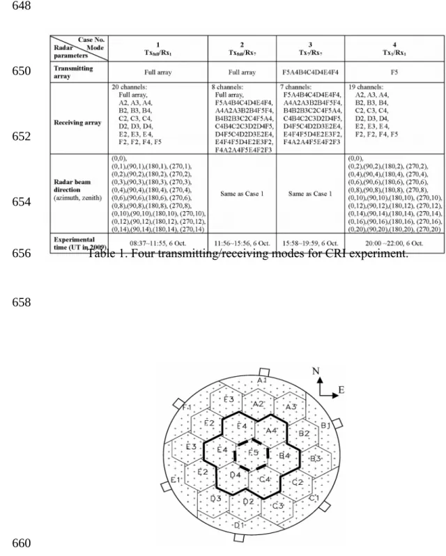
In this study, four CRI experiments with different combinations of antenna groups for reception, which yield different radar beam weighting effects, were carried out; Table 1 lists the radar beam direction and transmitting/receiving subarrays
employed in the experiments, where the terms Txfull, Tx7 (Rx7) and Tx1 (Rx1) represent
transmission (reception) with full array, seven, and one antenna groups, respectively. However, some data were not shown in this study: (1) the data received by full array in cases 1 and 2, which is not required for CRI; (2) the data received by the radar beam directions at off-zenith angles of 12o and 14o in cases 1-3, which yield very
small brightness values around zenith so that the values of e disperse greatly; (3) the
data received by the radar beam directions at off-zenith angles of 10o and 14o in case
4, which are not presented for saving space.
In all experiments, radar pulse length was 1 s, sampling step was 150 m, and sampling time was 0.1184 s. 256 raw data points were taken for an estimate of cross-correlation function between a pair of receivers.
B. Capon’s method used with CRI
Although several imaging algorithms can be chosen for estimating CRI bright-ness, the Capon method is suitable for distributed target like refractivity irregularities in the atmosphere as compared with the MUSIC method, and it consumes less compu-tation time as compared with the maximum entropy algorithm. The Capon method is also one of the most favorable approaches in synthetic-aperture-radar (SAR) 146 148 150 152 154 156 158 160 162 164 166 168 170 172 174 176 178 180 182
tomography [23]-[25].
The imaging process with the Capon method can be carried out in both time and Doppler frequency domains; the latter can show the brightness distribution for various Doppler frequency components. In this study, the time-domain calculation was exe-cuted to estimate the angular brightness B(k):
e R e 1 1 ) ( H B k , (5a)
where k=(2π/λ)[sinθsinφ, sinθcosφ, cosθ], which is the wavenumber vector in the direction of inspection. λ is the radar wavelength; θ and φ are, respectively, the zenithal and azimuthal angles. Matrix e is a complex weight with the form of [ ejk•D1
ejk•D2 … ejk•Dn ]T, where D
n denotes the central position vector of the nth receiving
antenna group. The superscripts H, T, and -1 represent, respectively, Hermitian operator, transposition, and inverse of matrix. R is a matrix defined as
nn
n
n
n
n
R
R
R
R
R
R
R
R
R
...
.
. .
.
...
...
2
1
2
22
21
1
12
11
R
, (5b)where Rij is the zero-lag cross-correlation function of the signals received by receivers i and j.
C. Calibration results
With (5), the CRI data of a pair of symmetrically oblique radar beams were processed with an angular step of 0.25o in both zonal and meridional directions, and then the
brightness values imaged between -2o and 2o zenith along the line of the tilted radar
beams were used with (4) to estimate an effective beamwidth (e). The threshold of
SNR, 0.0625 or -12dB, was given for performing the computation or not. It should be mentioned that the value of e varies slightly with the angular extent of brightness
values used; a detailed discussion on this is given in Section IV.
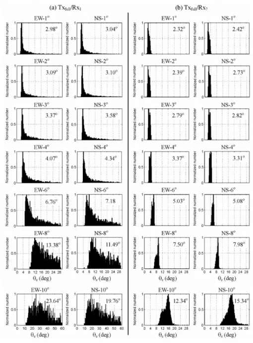
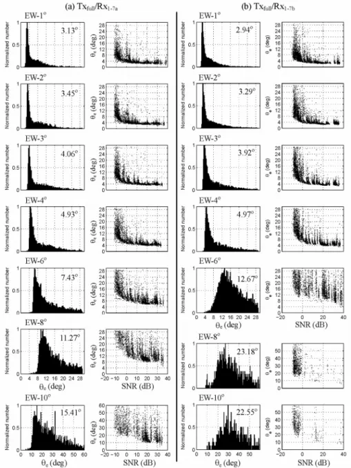
Figures 2 and 3 show the histograms of e for the beam pairs along, respectively,
184 186 188 190 192 194 196 198 200 202 204 206 208 210
east-west (EW) and north-south (NS) directions in the experiments 1-4, using the data of 60 sampling range gates that are within the height interval between ~2 and ~11 km. First, we can observe some features: (1) for each Tx/Rx mode, the histograms of e in
EW and NS directions are similar; (2) e becomes larger for the oblique beam tilted to
a larger off-zenith angle; (3) different Tx/Rx modes result in various characteristics of the histogram of e. We discuss these features in more detail in the following.
In Figure 2(a), the distribution of e is not Gaussian-shaped and in general, a
larger value of e corresponds to a lower SNR (shown later in Figure 4). The mean
peak location of the distribution, as indicated in each panel, was estimated in the following two steps: (1) mean (e ) and standard deviation () of the distribution was
computed first, (2) the values of e smaller than e were adopted to compute
again a mean and a standard deviation of e. In this way, the resultant mean value of
e can be closer to the apparent peak location of the distribution. To reduce the
influence of low-SNR data further, only the data of the lowest 20 sampling range gates under the condition of SNR>0 dB were used. Note that the qualifications of estimating the mean value of e are stricter than those of showing the histogram of e
so that the mean value of e (termed the likely value of e hereafter) can be closer to
the beamwidth of without noise.
Apparently, the likely value of e varies with the off-zenith angle of the radar
beam direction. Nevertheless, the likely values of e obtained from the pairs of radar
beams tilted to the off-zenith angles smaller than 4o are very close (between ~3o~4o).
As the off-zenith angle of the radar beam direction increases, the likely value of e
becomes larger as well (notice the abscissa of the lowest panel has different scale from the others). Readers may have noticed that differences in the likely values of e
between EW and NS directions are larger for the radar beams tilted to the off-zenith angles of 8o and 10o. We attribute it to two factors: (1) the lower-intensity echoes
returning from the region closer to the edge of the radar beam, which leads to a larger statistical uncertainty in calculation, and (2) the grating pattern arising from finite spatial distance between receiving antenna groups. The second attribution is discussed in Section IV. In spite of the slightly difference in e between EW and NS directions,
the calibration results indicate that the likely value of e varies with the off-zenith
angle of the radar beam direction.
Based on the likely values of e estimated above and from the concept proposed
in Section II, it is inferred that if the radar beam weighting function, exp(-sin2/sin2 o)
or exp[-(sin-sinT)2/sin2o], is assumed, the value of o, represented by the e
estimated, should increase with the off-beam-direction angle. Quantitatively, Figure 2(a) suggests that the likely value of e vary from ~3o to ~20o for the
off-beam-direction angles between 0o and 10o. It is also indicated that the commonly mentioned
212 214 216 218 220 222 224 226 228 230 232 234 236 238 240 242 244 246 248
half-power half-width (HPHW) could be between 3o~4o for the Tx
full/Rx1 mode (full
array for transmission and one antenna group for each receiving channel), according to the results of the radar beam pairs at off-zenith angles smaller than 4o. It deserves a
mention that in the use of full array for transmission and reception, the modeled HPHW is ~1.87o [26], which is smaller than the likely value of
e obtained here. Such
difference in HPHW is owing to the use of the receiving array in the present experiment; that is, only one antenna group, not the full array, was used for each receiving channel, causing the effective HPHW larger than the modeled HPHW of full array.
Another observation in Figure 2(a) is the more dispersive distribution of e for
the radar beam pair with a larger off-zenith angle. Such feature is associated mainly with low SNR of the radar echoes for a more oblique radar beam as well as poorer quality of the brightness value located far from the radar beam center. If a larger antenna array is used in receiving the echoes, SNR can be increased and the data quality can be raised. As a result, the distribution of e can be more concentrated.
Figure 2(b) shows such a case, where the radar echoes of seven antenna groups were combined for output of each receiving channel (denoted as Rx7). Compared with
Figure 2(a), the distributions of e in Figure 2(b) are indeed more concentrated. In
addition, the combination of seven antenna groups for output of each receiving channel leads to a narrower beamwidth as compared with the use of one antenna group; this characteristic can also be revealed according to the likely values of e
indicated in Figure 2(b).
Figure 2 suggests a positive dependence of effective beamwidth on off-beam-direction angle. Two more experiments for supporting this conclusion are presented in Figure 3.
Figure 3(a) shows the histograms of e resulting from using the same antenna
groups for transmission and receptionthe Tx7/Rx7 mode; the histograms of e are
very similar to Figure 2(b). However, the values of e shown here are slightly larger
than those in Figure 2(b) for the radar beam having an off-zenith angle smaller than 4o, which can be attributed to the use of seven antenna groups for transmission (Tx
7)
that yields a larger transmitting beamwidth. The modeled HPHW of the Tx7/Rx7 mode
is ~3.46o [26]; therefore, the effective beamwidths obtained from the radar beams
tilted to the off-zenith angles smaller than 4o are very close to the modeled one. As the
off-zenith angle of radar beam increases, the effective beamwidth increases
accordingly and thereby indicates that the modeled beamwidth is suitable for use only around the vicinity of the radar beam center.
The fourth experiment employed only one antenna group for transmission and for output of each receiving channel. Such use of Tx/Rx mode is expected to result in 250 252 254 256 258 260 262 264 266 268 270 272 274 276 278 280 282 284 286
an effective beamwidth much larger than the previous three experiments, as
demonstrated in Figure 3(b). As shown, the likely values of e are 9.63o and 10.96o for
the beam pair with tilt angle of 2o zenith, which are very close to the modeled HPHW:
~10.24o. As the off-zenith angle of radar beam increases, the likely value of
e
becomes larger and the distribution of e is getting widespread, like that in Figure
2(a).
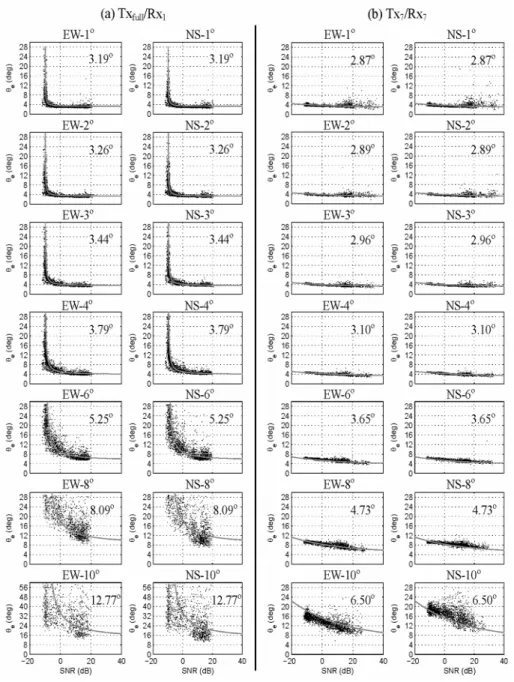
To see the influence of SNR on the effective beamwidth, we present the scatter diagrams of e versus SNR in Figure 4 for the two modes of Txfull/Rx1 and Tx7/Rx7, in
which the curve shown in each panel is a fitting result that is explained later.
Apparently, the variations of e with SNR are different between the two Tx/Rx modes
at very low SNR: the e of the Txfull/Rx1 mode gets larger more quickly than the
Tx7/Rx7 mode. On the other hand, e approaches to some values as SNR is getting
large. Based on these observations, it is possible to find a set of equations for fitting the relationship between e and SNR at different off-beam-direction angles. Taking
the Txfull/Rx1 mode as an example and assuming a symmetric radar beam pattern in
azimuthal direction, the process is as follows:
1) Give a set of HPHW for all beam pairs that can indicate the effective beamwidths at infinite SNR. Such a value set, denoted as oe hereafter, can be assigned
approximately by extending the dependent relationship in Fig. 4 to very high SNR, which should be smaller than the likely values of e indicated in Figures 2-3.
For example, if the set of oe=[2.80o, 3.00o, 3.50o, 4.00o, 5.50o, 8.50o, 12.50o] are
given for the beam pairs tilted to the zenith angles of T=[1o, 2o, 3o, 4o, 6o, 8o, 10o],
then a cubic curve,
2 3 T 1 oe c c , (6)
is capable of depicting the relationship between oe and T. Figure 5(a) shows the
fitting result, with the constants c1≒0.0096 and c2≒3.1803. Such obtained cubic
equation can be employed to estimate effective beamwidths at infinite SNR for various off-beam-direction angles, by regarding the off-zenith angle T as the
off-beam-direction angle of a radar beam.
2) Substitute the value of oe, estimated with (6) for an off-beam-direction angle (i.e.,
the variable T), into the following equation which describes the relationship
between e and SNR (in dB):
oe 4 2 3 e 10 SNR c c oe , (7) 288 290 292 294 296 298 300 302 304 306 308 310 312 314 316 318 320 322 324
where c3≒1.4751 and c4≒-9.7430 for the fitting curves shown in Figure 4(a).
Notice that c1c4 are constants resulting from fitting processes.
Eqs. (6) and (7) are empirical and they are certainly not unique. In addition, in the use of (7) SNR must be larger than -10 dB to avoid a negative e. In view of this, other
expressions which can describe well the relationship between e and SNR can also be
employed.
With the same process, the fitting curve for the Tx7/Rx7 mode can be obtained,
too. First, by giving a value set of oe=[2.80, 2.90, 3.00, 3.10, 3.60, 4.50, 6.00] for the
beam pairs tilted to the zenith angles of T=[1o, 2o, 3o, 4o, 6o, 8o, 10o], the cubic curve
(6) is used again to find a relationship between oe and T. The result is shown in
Figure 5(b), where c1≒0.0036 and c2≒2.8655. Second, use the following expression
to characterize the relationship between e and SNR (in dB):
oe o o oe e a c SNR exp[ ] 8 . 2 , (8)
where ao=3.0 and co= 0.03. Like (7), Eq. (8) is empirical and not unique, but it can yet
be regarded as one of usable expressions, as demonstrated by the fitting curves shown in Figure 4(b).
The fitting curves shown in Figure 4(b) fit the data well except the case of NS-10o. As readers can see, the values of
e in the panel of NS-10o are apparently larger
than those in the panel of EW-10o, which has been found in the likely values of e
shown in Figures 3(a). The reason for this discrepancy could be the grating lobe pattern of CRI; it is discussed in Section IV.
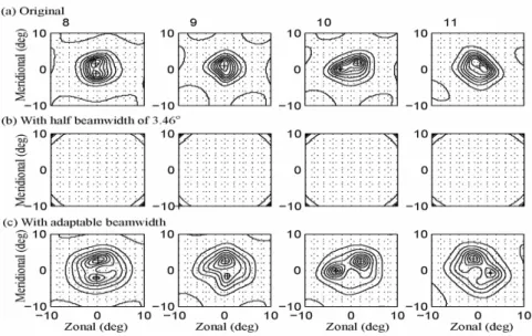
D. Comparison between original and corrected CRI results
Fig. 6 shows some original and corrected imaging results, presented by contour lines, of the Tx7/Rx7 mode. The imaged brightness values were self-normalized each
plot. It is apparent that the contour map corrected by a fixed beamwidth is unrealistic (Fig. 6(b)), which is of no use. By contrast, the contour map rectified with an
adjustable beamwidth reveal some noticeable features. For example, the raw contour maps reveal double–center pattern at gates 8 and 10, which also appear in the
corrected maps but with a larger separation between the two centers. On the other hand, the cases of single echo center observed at gates 9 and 11 in the raw maps change to the situation of double echo centers. Statistics showed that the failure rate arising from modification of brightness value was only ~0.43%, and moreover, about 326 328 330 332 334 336 338 340 342 344 346 348 350 352 354 356 358 360
14% of the single-center cases turned into multiple-center situations. In view of this, correction of radar beam weighting effect on the CRI brightness is indeed crucial sometimes; it may revise the number and locations of echo centers, the brightness width, and then reveal some concealed information. A further investigation on whether the double-center situation is related to some kind of atmospheric
characteristic is beyond the scope of this study, but it has been shown that wavy layer structures can be one of the causes of the double-center situation [9], [17].
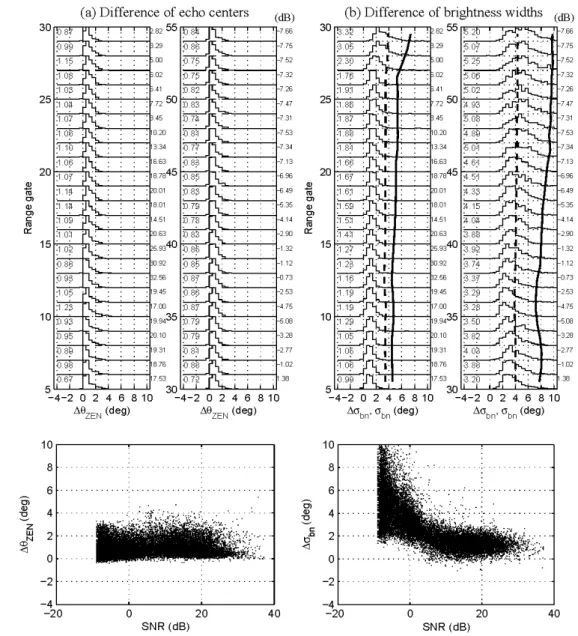
A general influence of radar beam weighting correction on echo center and brightness width can be investigated from statistical aspect. Figure 7 shows one of the experiments: Tx7/Rx7 mode. In showing Figure 7, only the cases with single center
were taken for avoiding miscomparison between different echo regions when double-center situation occurs, and moreover, the lowest threshold of SNR was -9 dB. Positive difference means that the corrected zenith angle of echo center (i.e., DOA) and brightness width are larger than the original ones. Notice that the two numbers given for each range gate are means of, respectively, SNRs and differences of DOAs or brightness widths, respectively. Also notice that the brightness width estimated here is the mean of the two half-widths of the brightness distribution along its major and minor axes.
The histograms (stair curves) shown in Figure 7(a) reveal that the corrected zenith angles of echo centers were larger than the original ones by ~1o, and the mean
difference was ~0.75o and did not vary with SNR for the SNR larger than -9 dB, as
indicated in the scatter diagram. Such a difference in the location of echo center could be crucial sometimes. For example, in the study of long-term mean vertical wind using a VHF atmospheric radar [17], an error of 0.75o in the location of echo center
can induce a bias of ~13.09 cm/s in vertical velocity when the horizontal wind is 10 m/s; this is a quite large value for the mean vertical velocity of the atmosphere.
The corrected brightness widths were also larger than the original ones, as shown in Figure 7(b), where the profiling curves are the means of original (dashed) and corrected (solid) brightness widths (bn), respectively, and the stair curves indicate the
distributions of differences in brightness width (bn). The scatter diagram, as shown
in the lower plots, demonstrates that the value of bn was dependent on SNR, which
is different from the characteristic of echo center difference. For SNR> ~6 dB, the values of bn were mostly between 0o and 2o; for SNR< ~6 dB, however, bn
increased noticeably. In view of this, it would be better to take the variation of brightness width with SNR into account when the brightness width is applied to deriving atmospheric parameters. For example, the brightness width is associated with aspect sensitivity of the echoing irregularities, and therefore the radar beam weighting effect on brightness distribution need to be removed in advance for a more proper 362 364 366 368 370 372 374 376 378 380 382 384 386 388 390 392 394 396 398
estimate of aspect angle of the irregularities. This point can be demonstrated partly from a comparison between the two profiling curves in Figure 7(b). As shown, the mean of the original brightness widths (dashed curve) is almost constant along range gate (or altitude); by comparison, the altitudinal variation of the corrected brightness width (solid curve) is visible, and moreover, the profiling curve for the corrected brightness widths reveals a height interval with smaller brightness widths (higher aspect sensitivity), where was located around 35 range gate or 6.3 km, in the vicinity of tropopause height. Without correction, however, the original brightness width could hardly disclose it.
IV. Discussion
Figures 2-4 reveal that different Tx/Rx modes result in different distributions of e. It is worthy of a further examination on factors of limitation or usability of the
calibration approach, for example, the number of receivers, the baseline length between receiving antenna groups, angular extent of brightness distribution adopted, and so on. First, we take the experiment of Txfull/Rx1 mode for the studies of the two
factors: number of receivers and baseline length between receiving antenna groups, as shown in Figure 8.
Figure 8(a) shows the calibration result in the east-west direction, with seven receiving antenna groups: F5, A4, B4, C4, D4, E4, and F4 (denoted as Rx1-7a). The
only difference between the two modes of Txfull/Rx1 and Txfull/Rx1-7a is the number of
receivers. Compared with the Txfull/Rx1 mode (Figure 2(a) and 4(a)), the aspect of e
histogram shown here remains unchanged although the distribution of e is more
dispersive. The likely values of e for the beam pairs EW-1o~6o are close to the ones
obtained in Figure 2(a); for the beam pairs EW-8o and EW-10o, however, their likely
values of e are different more from those of Figure 2(a).
A further examination is exhibited in Figure 8(b), with another set of receiving antenna groups: F5, A2, B2, C2, D2, E2, and F2 (denoted as Rx1-7b). Note that the
baseline length of the Rx1-7b mode is about the double of the Rx1-7a mode. Compared
with Figure 8(a), the distribution of e is more dispersive and it indicates that the
cali-bration approach is workable only for the beam pairs EW-1o~4o. The likely values of
e for the beam pairs EW-6o~10o get larger and they are unreliable according to the
scattering diagrams of e and SNR. Such consequences could be attributed to a longer
baseline length between receiving antenna groups, which result in a different grating lobe pattern from those of Rx1 and Rx1-7a receiving modes. For comparison, three
typi-cal grating lobe patterns, mapped in contour lines, for the three receiving modes: Rx1,
400 402 404 406 408 410 412 414 416 418 420 422 424 426 428 430 432 434 436
Rx1-7a, and Rx1-7b, are displayed in Figure 9. For the Rx1 or Rx1-7a receiving mode, the
grating lobe pattern shows that the folding/aliasing angle is ~22o; for the Rx
1-7b
receiv-ing mode, however, the foldreceiv-ing/aliasreceiv-ing angle is only ~11o. As a result, the duplicated
imitations around the central one degrade gradually the calibration result of the Rx1-7b
receiving mode for the beam pair with tilt angle larger than ~5.5o.
The grating lobe pattern can also explain, to some degree, the unsymmetrical cal-ibration results in the east-west and north-south directions for the radar beam with a larger tilt angle. That is, the grating lobe pattern of the Txfull/Rx1 mode reveals some
imitations aligned nearly in north-south direction, which will give a larger error to cal-ibration result than in the east-west direction for the radar beam with the tilt angle of 10o. This also occurs in the Tx
full/Rx7, Tx7/Rx7, and Tx1/Rx1 modes for the baseline
lengths and orientations of their receiving antenna groups are the same as the Tx -full/Rx1 mode. In view of this, the calibration in the east-west direction is more reliable
for the receiving configurations employed here.
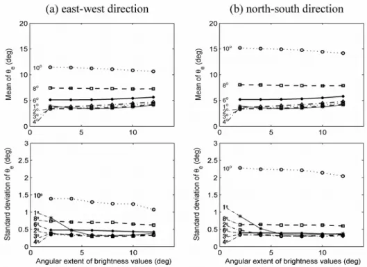
Finally, we discuss the use of brightness values within different angular extents for calibration. Taking the Tx7/Rx7 mode as an example, Figure 10 shows the
respective means (upper plots) and standard deviations (lower plots) of e for 2o, 4o,
6o, 8o, 10o, and 12o angular extents, where computation of mean, namely, the the likely
value of e was carried out with the same criteria used in Figures 2 and 3. As seen, the
means of e vary slightly with angular extent, which is a consequence of averaging
from different effective beamwidths within different angular extents.
According to the argumentation of the proposed calibration approach, using the imaged brightness within a smaller angular extent can result in a more representative value of e at a specific off-beam-direction angle, while use of the imaged brightness
within a larger angular extent gives a value of e that is a mean within a wider range
of off-beam-direction angles. In view of this, the result of 2o angular extent is
expected to be the optimal. Nevertheless, for the beam pairs with tilt angles of 1o4o
zenith the resultant features of 2o angular extent are slightly different from the other
angular extents; that is, with 2o angular extent the mean
e obtained from the beam
pair having the tilt angle of 1o zenith (*) is slightly larger than those of the other three
beam pairs, but it is not the case for the use of larger angular extents. Moreover, with 2o angular extent the standard deviation of
e for the beam pair with tilt angle of 1o
zenith is apparently larger than others except the beam pair of 10o zenith, as shown in
the bottom plots of Figure 10. Based on these statistical estimates, the use of brightness values within 4o angular extent is suitable for calibration, which can avoid
a worse product from a very small angular extent, and can also conform the argumentation of the calibration approach to the utmost to provide a representative value of e. 438 440 442 444 446 448 450 452 454 456 458 460 462 464 466 468 470 472 474
The cause of the worse product from very small angular extent could be attributed to statistical error, according to the estimate of standard deviation.
V. Conclusions
In this paper, an approach is proposed to mitigate the radar beam weighting effect on the brightness distribution imaged by the coherent radar imaging (CRI) technique of VHF atmospheric radar. It is then expected to yield more suitable estimates of echo center and brightness width from the modified brightness
distribution. The approach uses several pairs of symmetrically oblique radar beams to determine an effective weighting pattern of the radar beam. Differing from a fixed radar beam pattern commonly used, such obtained weighting pattern is adaptive to signal-to-noise ratio (SNR) and transmitting/receiving (Tx/Rx) mode.
Four experiments with the MU radar in Japan were carried out to validate the proposed approach. It showed that different Tx/Rx modes give different
characteristics of effective beamwidths. We have demonstrated that the characteristics of effective beamwidths are related to the radar beam weighting pattern of Tx/Rx mode, the baseline length of receiving antenna groups, and the SNR of radar echoes. Moreover, error estimation of effective beamwidth was also carried out with different angular extents of brightness values in calibration process. The limitation and
usability of the proposed calibration approach are thereby clarified.
The experimental results of the Tx7/Rx7 mode are exhibited in more detail in this
paper. It is demonstrated from statistics that the zenith angles of the corrected echo centers were mostly larger than the original ones, and the mean difference was ~0.75o.
On the other hand, the corrected brightness widths were larger than the original ones by up to several degrees, and the difference between the corrected and original brightness widths increased with decreasing SNR, which is different from the behavior of echo center.
With the proposed approach and based on the present studies, it is expected that measurements of some atmospheric parameters with CRI can be improved, for example, aspect sensitivity of refractivity irregularities, bias of mean vertical velocity measured by VHF atmospheric radars, tilt angle of layer structure, and so on.
Validation of improvement in the above parameters with CRI needs more examinations and larger space of presentation; we leave it to follow-up studies. Acknowledgements
This work was supported by the National Science Council of ROC (Taiwan) through 476 478 480 482 484 486 488 490 492 494 496 498 500 502 504 506 508 510 512
grants NSC98-2111-M-270-001 and NSC99-2111-M-270-001-MY2, and also supported by the International Collaborative Research Program of MU radar (Ref. No.: 21MU-A-43). The MU radar is operated by the Research Institute for Sustainable Humanosphere, Kyoto University, Japan.
References
[1] J. Röttger and R. A. Vincent, “VHF radar studies of tropospheric velocities and ir-regularities using spaced antenna technique,” Geophys. Res. Lett., vol. 5, no. 11, pp. 917-920, doi:10.1029/GL005i011p00917, 1978.
[2] D. T. Farley, Ierkic, H. M., and Fejer, B. G, “Radar interferometry: A new tech-nique for studying plasma turbulence in the ionosphere,” J. Geophys. Res., vol. 86, no. A3, pp. 1467–1472, doi:10.1029/JA086iA03p01467, 1981.
[3] J. Capon, “High-resolution frequency-wavenumber spectrum analysis,” Proc. IEEE, vol. 57, no. 8, pp. 1408-1418, 1969.
[4] D. L. Hysell, “Radar imaging of equatorial F region irregularities with maximum entropy interferometry,” Radio Sci., vol. 31, no. 6, pp. 1567-1578,
doi:10.1029/96RS02334, 1996.
[5] D. L. Hysell and R.F. Woodman, “Imaging coherent backscatter radar observa-tions of topside equatorial spread F,” Radio Sci., vol. 32, no. 6, pp. 2309-2320, doi:10.1029/97RS01802, 1997.
[6] R. D. Palmer, S. Gopalam, T.-Y. Yu, and S. Fukao, “Coherent radar imaging us-ing Capon’s method,” Radio Sci., vol. 33, no. 6, pp. 1585-1598, doi:10.1029/98RS02200, 1998.
[7] M. C. Hélal, H. Luce, and E. Spano, “Radar imaging and high-resolution array processing applied to a classical VHF-ST profiler,” J. Atmos. Solar-Terr. Phys., vol. 63, pp. 263-274, 2001.
[8] R. F. Woodman, “Coherent radar imaging: Signal processing and statistical prop-erties,” Radio Sci., vol. 32, no. 6, pp. 2372–2391, doi:10.1029/97RS02017, 1997. [9] T.-Y. Yu, R. D. Palmer, and P. B. Chilson, “An investigation of scattering
mecha-nisms and dynamics in PMSE using coherent radar imaging,” J. Atmos. Solar Terr. Phys., vol. 63, pp. 1797–1810, 2001.
[10] P. B. Chilson, T.-Y. Yu, R. D. Palmer, and S. Kirkwood, “Aspect sensitivity measurements of polar mesosphere summer echoes using coherent radar imaging,” Ann. Geophys., vol. 20, pp. 213–223, 2002.
[11] D. L. Hysell, M. Yamamoto, and S. Fukao, “Image radar observations and theory of Type I and Type II quasi-periodic echoes,” J. Geophys. Res., vol. 107, no. A11, 1360, doi:10.1029/2002JA009292, 2002. 514 516 518 520 522 524 526 528 530 532 534 536 538 540 542 544 546 548 550
[12] D. L. Hysell, M. F. Larsen, and Q. H. Zhou, “Common volume coherent and incoherent scatter radar observations of mid-latitude sporadic E-layers and QP echoes,” Ann. Geophys., vol. 22, pp. 3277-3290, 2004.
[13] B. L. Cheong, M.W. Hoffman, R. D. Palmer, S. J. Frasier, and F. J. Lopez-Dekker, “Pulse pair beamforming and the effects of reflectivity field variation on imaging radars,” Radio Sci., vol. 39, no. 3, RS3014, doi:10.1029/2002RS002843, 2004.
[14] J. L. Chau and D. L. Hysell, “High altitude large-scale plasma waves in the equa-torial electrojet at twilight,” Ann. Geophys., vol. 22, pp. 4071–4076, 2004.
[15] R. D. Palmer, B. L. Cheong, M. W. Hoffman, S. J. Fraser, and F. J. López-Dekker, “Observations of the small-scale variability of precipitation using an imaging radar,” J. Atmos. Ocean. Technol., vol. 22, pp. 1122–1137, 2006
[16] M.-Y. Chen, T.-Y. Yu, Y.-H. Chu, W. O. J. Brown, and S. A. Cohn, “Application of Capon technique to mitigate bird contamination on a spaced antenna wind profiler,” Radio Sci., vol. 42, no. 6, RS6005,
doi:10.1029/2006RS003604, 2007.
[17] J.-S. Chen, G. Hassenpflug, and M. Yamamoto, “Tilted refractive-index layers possibly caused by Kelvin–Helmholtz instability and their effects on the mean vertical wind observed with multiple-receiver and multiple-frequency imaging techniques,” Radio Sci., vol. 43, no. 1, RS4020, doi:10.1029/2007RS003816, 2008.
[18] J.-S. Chen, P. Hoffmann, M. Zecha, and C.-H. Hsieh, “Coherent radar imaging of mesosphere summer echoes: Influence of radar beam pattern and tilted structures on atmospheric echo center,” Radio Sci., vol. 43, no. 4, RS1002, doi:10.1029/2006RS003593, 2008.
[19] T.-Y. Yu, “Radar studies of the atmosphere using spatial and frequency diver-sity,” Ph.D. thesis, University of Nebraska-Lincoln, 2000.
[20] W. K. Hocking, R. Rüster, and P. Chechowsky, “Absolute reflectivities and as-pect sensitivities of VHF radio wave scatterers measured with the SOUSY radar,” J. Atmos. Terr. Phys., vol. 48, pp. 131–144, 1986.
[21] J.-S. Chen and M. Zecha, “Multiple-frequency range imaging using the OSWIN VHF radar: Phase calibration and first results,” Radio Sci., vol. 44, no. 1, RS1010, doi:10.1029/2008RS003916, 2009.
[22] G. Hassenpflug, M. Yamamoto, H. Luce, and S. Fukao, “Description and demonstration of the new Middle and Upper atmosphere Radar imaging system: 1-D, 2-D and 3-D imaging of troposphere and stratosphere,” Radio Sci., vol. 43, RS2013, doi:10.1029/2006RS003603, 2008.
[23] P. Lo pez-Dekker and J. J. Mallorqui, “Capon- and APES-Based SAR Process-552 554 556 558 560 562 564 566 568 570 572 574 576 578 580 582 584 586 588
ing: Performance and Practical Consideration,” IEEE Trans. Geosci. Remote Sens, vol. 4, no. 5, pp. 2388-2402, 2010.
[24] Z. S. Liu, H. Li, and J. Li, “Efficient implementation of Capon and APES for spectral estimation,” IEEE Trans. Aerosp. Electron. Syst., vol. 34, no. 4, pp. 1314–1319, Oct. 1998.
[25] F. Lombardini and A. Reigber, “Adaptive spectral estimation for multibaseline SAR tomography with airborne L-band data,” in Proc. IEEE IGARSS, vol. 3, pp. 2014–2016, 2003.
[26] T. E. VanZandt, G. D. Nastrom, J. Furumoto, T. Tsuda, and W. L. Clark, “A dual-beamwidth radar method for measuring atmospheric turbulent kinetic en-ergy,” Geophys. Res. Lett., vol. 29, no. 12, 10.1029/2001GL014283, 2002.
Table Captions
Table 1. Four transmitting/receiving modes for CRI experiment.
Figure Captions
Figure 1. Antenna array configuration of the MU VHF radar. Twenty five antenna groups are denoted from A1 to F5. The radius of antenna field is about 55 m.
Figure 2. Histogram of effective beamwidth (e) obtained from two symmetrically
oblique radar beams. (a) Txfull/Rx1 mode, and (b) Txfull/Rx7 mode. The value given
in each panel is the mean peak location of the histogram estimated from the lowest 20 sampling range gates and under the condition of SNR>0 dB.
Figure 3. Same as Fig. 2, but for (a) Tx7/Rx7 mode, and (b) Tx1/Rx1 mode.
Figure 4. Scatter diagram of effective beamwidth (e) versus signal-to-noise ratio
(SNR). The curves in (a) and (b) result from Eqs. (7) and (8), respectively. The value given in each panel is the effective beamwidth at infinite SNR, estimated with (6).
Figure 5. Relationship between effective beamwidth and off-zenith angle of the radar beam direction for the condition of infinite SNR. The fitting curves result from (6).
Figure 6. Contoured CRI brightness distribution (self-normalized): (a) original, (b) modified with the half beamwidth of 3.46o, and (c) modified with adaptable
beamwidth. Plus sign indicates the mean location of echo center. Contour levels are ten.
Figure 7. Differences in (a) zenith angles of echo centers (ZEN) and (b) brightness
widths (bn) between corrected and original CRI brightness distributions of the
590 592 594 596 598 600 602 604 606 608 610 612 614 616 618 620 622 624 626
Tx7/Rx7 mode. The profiling curves show the means of original (dashed) and
corrected (solid) CRI brightness widths. Scatter diagrams show the variations of ZEN and bn, respectively, versus SNR. Only the data with SNR > -9 dB were
taken.
Figure 8. (a) Histogram of effective beamwidth (e) and scatter diagram of e versus
SNR in the east-west direction for case 1, but use only seven of the 19 receivers for calibration (receiving antenna groups: F5, A4, B4, C4, D4, E4, F4). The mode is termed Txfull/Rx1-7a. (b) is similar to (a), but obtained with another set of
receiving antenna groups: F5, A2, B2, C2, D2, E2, F2, and denoted as Txfull/Rx1-7b
mode.
Figure 9. The Capon grating lobe patterns for the Txfull/Rx1, Txfull/Rx1-7a, and
Txfull/Rx1-7b receiving modes, mapped in contour lines (self-normalized). Radar
beam weighting effect is not removed. Plus sign indicates the mean location of echo center. Contour levels are five.
Figure 10. Error estimations of effective beamwidths (e) for the beam pairs with tilt
angles of 1o, 2o, 3o, 4o, 6o, 8o, and 10o, respectively. The angular extents of
brightness values adopted for computation are 2o, 4o, 6o, 8o, 10o, and 12o. (a) The
results of the Tx7/Rx7 mode in the east-west direction. The upper plot is the mean
of e, and the lower plot is the standard deviation of e. (b) Same as (a), but in the
north-south direction. 628 630 632 634 636 638 640 642 644 646
Table 1. Four transmitting/receiving modes for CRI experiment.
Figure 1. Antenna array configuration of the MU VHF radar. Twenty five antenna groups are denoted from A1 to F5. The radius of antenna field is about 55 m.
648 650 652 654 656 658 660 662 664
Figure 2. Histogram of effective beamwidth (e) obtained from two symmetrically
oblique radar beams. (a) Txfull/Rx1 mode, and (b) Txfull/Rx7 mode. The value given in
each panel is the mean peak location of the histogram estimated from the lowest 20 sampling range gates and under the condition of SNR>0 dB.
666
668 670
Figure 3. Same as Fig. 2, but for (a) Tx7/Rx7 mode, and (b) Tx1/Rx1 mode.
672
Figure 4. Scatter diagram of effective beamwidth (e) versus signal-to-noise ratio
(SNR). The curves in (a) and (b) result from Eqs. (7) and (8), respectively. The value given in each panel is the effective beamwidth at infinite SNR, estimated with (6). 676
Figure 5. Relationship between effective beamwidth and off-zenith angle of the radar beam direction for the condition of infinite SNR. The fitting curves result from (6).
Figure 6. Contoured CRI brightness distribution (self-normalized): (a) original, (b) modified with the half beamwidth of 3.46o, and (c) modified with adaptable
beamwidth. Plus sign indicates the mean location of echo center. Contour levels are ten. 680 682 684 686 688 690 692 694
Figure 7. Differences in (a) zenith angles of echo centers (ZEN) and (b) brightness
widths (bn) between corrected and original CRI brightness distributions of the
Tx7/Rx7 mode. The profiling curves show the means of original (dashed) and
corrected (solid) CRI brightness widths. Scatter diagrams show the variations of ZEN
and bn, respectively, versus SNR. Only the data with SNR > -9 dB were taken.
696 698 700
Figure 8. (a) Histogram of effective beamwidth (e) and scatter diagram of e versus
SNR in the east-west direction for case 1, but use only seven of the 19 receivers for calibration (receiving antenna groups: F5, A4, B4, C4, D4, E4, F4). The mode is termed Txfull/Rx1-7a. (b) is similar to (a), but obtained with another set of receiving
antenna groups: F5, A2, B2, C2, D2, E2, F2, and denoted as Txfull/Rx1-7b mode.
702
704 706 708
Figure 9. The Capon grating lobe patterns for the Txfull/Rx1, Txfull/Rx1-7a, and
Txfull/Rx1-7b receiving modes, mapped in contour lines (self-normalized). Radar beam
weighting effect is not removed. Plus sign indicates the mean location of echo center. Contour levels are five.
Figure 10. Error estimations of effective beamwidths (e) for the beam pairs with tilt
angles of 1o, 2o, 3o, 4o, 6o, 8o, and 10o, respectively. The angular extents of brightness
values adopted for computation are 2o, 4o, 6o, 8o, 10o, and 12o. (a) The results of the
Tx7/Rx7 mode in the east-west direction. The upper plot is the mean of e, and the
lower plot is the standard deviation of e. (b) Same as (a), but in the north-south
direction. 710 712 714 716 718 720 722 724