行政院國家科學委員會專題研究計畫 成果報告
日內報酬率波動性之微波分析
計畫類別: 個別型計畫 計畫編號: NSC91-2415-H-004-023- 執行期間: 91 年 08 月 01 日至 92 年 07 月 31 日 執行單位: 國立政治大學國際貿易學系 計畫主持人: 林信助 報告類型: 精簡報告 處理方式: 本計畫可公開查詢中 華 民 國 92 年 10 月 29 日
行政院國家科學委員會專題研究計畫成果報告
日內報酬率波動性之微波分析
Wavelet Analysis of Intraday Return Volatility
計畫編號:NSC
91-2415-H-004-023-
執行期限:2002 年 08 月 01 日至 2003 年 07 月 31 日
主持人:林信助
國立政治大學國際貿易學系
1. 摘要 在本研究計畫中,我們研究『台灣股 票發行量加權指數期貨』日內報酬率波動 性的行為。我們發現,該日內報酬率波動 性有類似於文獻中所提到的呈現明顯 U-型 變動的現象。我們採用 Andersen and Bollerslev (1997) 同時考慮『日內循環變動 因子』及『日間條件變異因子』的理論架 構,來探討報酬率日內波動性如何受到日 內循環變動因子的影響。所不同的是,我 們採用微波分析(Wavelet Analysis)來取代 Fourier Flexible Form (FFF),以過濾日內循環 變動因子。這麼做的好處是微波分析的結 果與時間上的頻率相互對應,具有明顯的 經濟涵意。這是其他多項式配適(polynomial fitting),包括 FFF,所不具備的性質。我們 發現,微波分析的確可以有效地過濾掉大 部分的日內循環變動因子。本研究有助於 日內報酬率條件變異數模型參數的穩健與 正確的估計,以及幫助我們對高頻率日內 報酬率波動性的性質有更進一步的瞭解。 關鍵詞: 日內波動性,微波分析。 AbstractIn this paper, we propose to examine the intraday volatility behavior of the Taiwan Stock Exchange Capitalization Weighted Stock Index (TAIEX) futures returns. Observing that the TAIEX futures return volatility exhibits the same U-shape patters as those reported in the literature, we adopt Andersen and Bollerslev (1997) stylized model, which allows interaction between the intraday periodicity and the interday conditional heteroscedasticity. The main thrust of this project is to replace Andersen and Bollerslev’s Fourier Flexible Form (FFF) filtration of the intraday periodicity with a wavelet filtration. Since all wavelet analysis correspond to frequencies in calendar time, the proposed wavelet filtration allows us to filter out intraday periodicity more appropriately, and hence contributes to our better understanding of the intraday volatility behavior.
Keywords: Intraday Periodicity, Wavelet
1. Introduction & Literature Review
With their distinct time-series properties, the advent of high-frequency data has also created new challenges to empirical work on return dynamics, see Andersen (2000). One such pronounced feature is that intraday return volatility often displays periodic pattern. Empirical evidence of this stylized fact can date back to, at least, Wood et al. (1985) and Harris (1986) who document the existence of a distinct U-shaped pattern in return volatility over the trading day, i.e. volatility is high at the open and at the close of trading and low in the middle of the day. More recent literature, Chan et al. (1991), Dacorogna et al. (1993), Andersen and Bollerslev (1997, 1998), Andersen et al. (2000), and Ederington and Lee (2001), continue to support such U-shaped volatility pattern, most notably in foreign exchange markets and equity markets.
Andersen and Bollerslev (1997) argue that these intraday periodic patterns are entirely alien to standard volatility models, and hence need to be accounted for be-fore any sensible inference can be derived. They demonstrate this point by showing that the temporal aggregation results for GARCH models developed by Nelson (1990, 1992), Drost and Nijman (1993) and Drost and Werker (1996) do not hold for the direct volatility estimates using raw data at various intraday frequencies. In order to disentangle the more interesting volatility behavior from the confounding intra-day patterns, Andersen and Bollerslev (1997) establish a stylized model that allows interaction between the interday volatility and the intraday periodicity, and suggest filtering out the intraday periodicity with the Fourier Flexible Form (FFF) introduced by Gallant (1981, 1982).
1.1. Andersen and Bollerslev’s Methodology
To explain the interaction between the intraday and the interday components, An-dersen and Bollerslev (1997) suggest the following stylized model for the intraday returns
Rt,n=
σtsnZt,n
N1/2 , (1.1)
where Rt,n denotes intraday continuously compounded return measured at the nth
intraday interval at date t, N denotes the number of high-frequency returns per day, σt is intended to capture the overall volatility level on day t, sn refers to a
determin-istic intraday periodic component, and Zt,n is an i.i.d. zero mean, unit variance error
term.1 Notice that when s
n = 1, ∀n, the daily return Rt ≡PNn=1Rt,n reverts to the
standard conditional heteroscedastic model. Within the stylized model in Eq. (1.1), Andersen and Bollerslev demonstrate two key points: (1) the presence of intraday periodic components reduces the overall level of the interday return autocorrelations
1
Rt,n can also be mean adjusted. However, since intraday average returns are practically
without affecting the autocorrelation pattern; (2) the periodicity may have strong impact on the autocorrelation pattern for the absolute intraday returns. Since such qualitative implications correspond well with empirical correlograms of intraday re-turns, Andersen and Bollerslev suggest the model in Eq. (1.1) as a good starting point for high frequency volatility modeling.
To further account for the empirical characteristics of intraday returns, Andersen and Bollerslev also allow the intraday periodic component, sn, to depend on the
char-acteristics of trading day, t, namely st,n. The flexible Fourier form (FFF), originally
proposed by Gallant (1981, 1982), is then used to filter out the periodicity component st,n. Specifically, define
xt,n ≡log(R2t,n) + log(N ) − log(bσ2t), (1.2)
where bσ2t denotes an a priori estimate of the daily volatility factor, which usually
involves estimating a volatility model from the GARCH family. Based on this defini-tion, the logarithmic periodic component, log(s2t,n), may be estimated from the linear
FFF-regression, xt,n= Q X q=0 δ0,q·nq+ P X p=1 [δc,p·cos(2πpn/N ) + δs,p·sin(2πpn/N )] + µt,n, (1.3)
where the tuning parameters, Q and P , determine the order of the Fourier expansion, δ0,q, δc,p, and δs,p are coefficients to be estimated, and the error term µt,n is i.i.d.
mean zero.2 By adopting the normalization scheme T−1PN n=1
P[T /N ]
t=1 st,n ≡ 1, the
normalized intraday periodic component for interval n on date t could be obtained by bst,n = T · exp(b xt,n/2) P[T /N ] t=1 PN n=1exp(bxt,n/2) , (1.4)
where T is the total number of observations, [T /N ] denotes the number of trading days in the sample. Consequently, we can define the filtered return as the following
e Rt,n ≡
Rt,n
bst,n
. (1.5)
Although flexible enough, it is usually difficult to attach any economic interpretation to such a nonparametric filtering procedure. Ideally, the filtering procedure should correspond to the frequency at which the phenomenon of interest are recurring. This motivates us to examine the applicability of the wavelet analysis, which is usually associated with a nature interpretation in terms of frequency in calendar time. We introduce the wavelet tool in the next section.
2
The choice of tuning parameters Q and P is an empirical question. Andersen et al. (2000) suggest choosing Q and P such that estimates for any additional δ0,q, δc,p,and δs,p coefficients are
2. Research Objectives
In this paper, we propose to study intraday return volatility behavior of the Tai-wan Stock Exchange Capitalization Weighted Stock Index (TAIEX hereafter) futures traded on the Taiwan Futures Exchange (TAIFEX). The intraday patterns of the TAIEX futures returns are strikingly similar to what were discovered in the aforemen-tioned literature. Since this is exactly the same issue that was examined in Andersen and Bollerslev (1997), we will follow their stylized model in this paper. However, instead of filtering the intraday periodicity by the FFF, we propose to implement the filtration by the wavelet analysis. The major advantage of using the wavelet analysis versus the FFF is that the wavelet filtration corresponds to a desired frequency in calendar time and hence attaches economic meaning to the filtration. This certainly does not come with the FFF, or any other polynomial filtering. After all, in the intra-day volatility context, what we really want is to filter out those periodic component recurring at daily frequency. It is therefore important to know what we leave out of the original data when applying any filtration procedure. Technically speaking, what we need to do is to project the original data series of interest onto a information subset (supported by wavelet functions) that corresponds to daily frequency.
3. Methodology
3.1. Wavelet Analysis
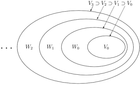
A wavelet is a “small wave” which has its energy concentrated in a short interval of time. The wavelet analysis allows researchers to decompose signals into a parsi-moniously countable set of basis functions at different time locations and resolution levels. Essentially, one can think of V0, W0, W1, W2, · · · as a partition of the
informa-tion set, as demonstrated in Figure 3.1. Indeed, what is of great interest to us is that each of these information subsets corresponds to a certain frequency in calendar time. It is this information decomposition that allows us to reconstruct variables of interest based on the subset of relevant information. Mathematically, this implies that the L2(R) space can be decomposed such that
L2(R) = V0⊕W0⊕W1 ⊕ · · ·. (3.1)
Each of those information subsets is spanned by a set of wavelet functions. More specifically, any discrete signal f (t) ∈ L2(R) can be written in terms of the father
and mother wavelets functions as the following:
f (t) = ∞ X k=−∞ αj0,kφj0,k(t) + X j≥j0 ∞ X k=−∞ βj,kψj,k(t), (3.2) where φj0,k(t) and ψj,k(t) are the father and the mother wavelet function, respectively;
Figure 3.1: Decomposition of Information . . . . . . . . . . . . . . . . . . . . . . . . . . . . . . . . . . . . . . . . . . . . . . . . . . . . . . . . . . . . . . . . . . . . . . . . . . . . . . . . . . . . . . . . . . . . . . . . . . . . . . . . . . . . . . . . . . . . . . . . . . . . . . . . . . . . . . . . . . . . . . . . . . . . . . . . . . . . . . . . . . . . . . . . . . . . . . . . . . . . . . . . . . . . . . . . . . . . . . . . . . . . . . . . . . . . . . . . . . . . . . . . . . . . . . . . . . . . . . . . . . . . . . . . . . . . . . . . . . . . . . . . . . . . . . . . . . . . . . . . . . . . . . . . . . . . . . . . . . . . . . . . . . . . . . . . . . . . . . . . . . . . . . . . . . . . . . . . . . . . . . . . . . . . . . . . . . . . . . . . . . . . . . . . . . . . . . . . . . . . . . . . . . . . . . . . . . . . . . . . . . . . . . . . . . . . . . . . . . . . . . . . . . . . . . . . . . . . . . . . . . . . . . . . . . . . . . . . . . . . . . . . . . . . . . . . . . . . . . . . . . . . . . . . . . . . . . . . . . . . . . . . . . . . . . . . . . . . . . . . . . . . . . . . . . . . . . . . . . . . . . . . . . . . . . . . . . . . . . . . . . . . . . . . . . . . . . . . . . . . . . . . . . . . . . . . . . . . . . . . . . . . . . . . . . . . . . . . . . . . . . . . . . . . . . . . . . . . . . . . . . . . . . . . . . . . . . . . . . . . . . . . . . . . . . . . . . . . . . . . . . . . . . . . . . . . . . . . . . . . . . . . . . . . . . . . . . . . . . . . . . . . . . . . . . . . . . . . . . . . . . . . . . . . . . . . . . . . . . . . . . . . . . . . . . . . . . . . . . . . . . . . . . . . . . . . . . . . . . . . . . . . . . . . . . . . . . . . . . . . . . . . . . . . . . . . ... . . . . . . . . . . . . . . . . . . . . . . . . . . . . . . . . . . . . . . . . . . . . . . . . . . . . . . . . . . . . . . . . . . . . . . . . . . . . . . . . . . . . . . . . . . . . . . . . . . . . . . . . . . . . . . . . . . . . . . . . . . . . . . . . . . . . . . . . . . . . . . . . . . . . . . . . . . . . . . . . . . . . . . . . . . . . . . . . . . . . . . . . . . . . . . . . . . . . . . . . . . . . . . . . . . . . . . . . . . . . . . . . . . . . . . . . . . . . . . . . . . . . . . . . . . . . . . . . . . . . . . . . . . . . . . . . . . . . . . . . . . . . . . . . . . . . . . . . . . . . . . . . . . . . . . . . . . . . . . . . . . . . . . . . . . . . . . . . . . . . . . . . . . . . . . . . . . . . . . . . . . . . . . . . . . . . . . . . . . . . . . . . . . . . . . . . . . . . . . . . . . . . . . . . . . . . . . . . . . . . . . . . . . . . . . . . . . . . . . . . . . . . . . . . . . . . . . . . . . . . . . . . . . . . . . . . . . . . . . . . . . . . . . . . . . . . . . . . . . . . . . . . . . . . . . . . . . . . . . . . . . . . . . . . . . . . . . . . . . . . . . . . . . . . . . . . . . . . . . . . . . . . . . . . . . . . . . . . . . . . . . . . . . . . . . . . . . . . . . . . . . . . . . . . . . . . . . . . . . . . . . . . . . . . . . . . . . . . . . . . . . . . . . . . . . . . . ... . . . . . . . . . . . . . . . . . . . . . . . . . . . . . . . . . . . . . . . . . . . . . . . . . . . . . . . . . . . . . . . . . . . . . . . . . . . . . . . . . . . . . . . . . . . . . . . . . . . . . . . . . . . . . . . . . . . . . . . . . . . . . . . . . . . . . . . . . . . . . . . . . . . . . . . . . . . . . . . . . . . . . . . . . . . . . . . . . . . . . . . . . . . . . . . . . . . . . . . . . . . . . . . . . . . . . . . . . . . . . . . . . . . . . . . . . . . . . . . . . . . . . . . . . . . . . . . . . . . . . . . . . . . . . . . . . . . . . . . . . . . . . . . . . . . . . . . . . . . . . . . . . . . . . . . . . . . . . . . . . . . . . . . . . . . . . . . . . . . . . . . . . . . . . . . . . . . . . . . . . . . . . . . . . . . . . . . . . . . . . . . . . . . . . . . . . . . . . . . . . . . . . . . . . . . . . . . . . . . . . . . . . . . . . . . . . . . . . . . . . . . . ... . . . . . . . . . . . . . . . . . . . . . . . . . . . . . . . . . . . . . . . . . . . . . . . . . . . . . . . . . . . . . . . . . . . . . . . . . . . . . . . . . . . . . . . . . . . . . . . . . . . . . . . . . . . . . . . . . . . . . . . . . . . . . . . . . . . . . . . . . . . . . . . . . . . . . . . . . . . . . . . . . . . . . . . . . . . . . . . . . . . . . . . . . . . . . . . . . . . . . . . . . . . . . . . . . . . . . . . . . . . . . . . . . . . . . . . . . . . . . . . . . . . . . . . . . . . . . . . . . . . . . . ... V0 W0 W1 W2 ¦ ¦ ¦ V3 ⊃V2 ⊃V1 ⊃V0 ¢ ¢® ¢ ¢ ¢® ¢ ¢ ¢ ¢ ¢® ¢ ¢ ¢ ¢ ¢ ¢ ¢®
j0 is a positive integer which represents the coarsest level of resolution chosen by
researchers; αj0,k =
R
f (t)φj0,k(t)dt, and βj,k =
R
f (t)ψj,k(t)dt are the expansion coefficients.3
To implement the wavelet analysis, Davidson et al. (1998) suggest a semi-nonparametric regression which avoids problems associated with the direct wavelet transform (DWT) and the wavelet shrinkage, namely the unequally-spaced data and the number of ob-servations being a power of 2. Lin and Stevenson (2001) adopt this procedure to examine the intraday relationship between the equity index and index futures prices in the cost-of-carry framework.
4. Results & Discussion
In this study, we only include transactions data for the entire year 2000 for the following reasons
1. Trades are the TAIFEX are electronically matched every 10 seconds since 12/06/1999. Before that, trades are only matched every 20 seconds.
3
The scale, j0, of the initial subspace is arbitrary. Due to the compact support property of
wavelets, the wavelet analysis is capable of capturing short lived, transient components of data in shorter time intervals, as well as capturing trends and patterns in longer time intervals. Consequently, the wavelet analysis is ideal for analyzing nonstationary data, which certainly include most economic and financial time series. In practice, it is usually chosen to represent the coarsest details of interest in a signal.
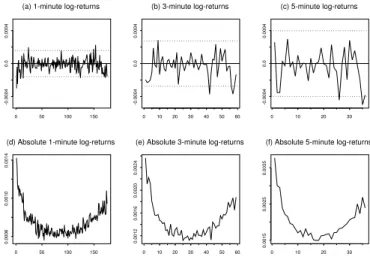
Figure 4.1: Intraday Average TAIEX Futures Returns
0 50 100 150
-0.0004
0.0
0.0004
(a) 1-minute log-returns
0 50 100 150
0.0006
0.0010
0.0014
(d) Absolute 1-minute log-returns
0 10 20 30 40 50 60 -0.0004 0.0 0.0004 (b) 3-minute log-returns 0 10 20 30 40 50 60 0.0012 0.0016 0.0020 0.0024
(e) Absolute 3-minute log-returns
0 10 20 30 -0.0004 0.0 0.0004 (c) 5-minute log-returns 0 10 20 30 0.0015 0.0025 0.0035
(f) Absolute 5-minute log-returns
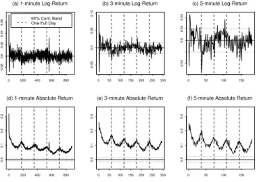
2. From 2001 onwards, the Taiwan Stock Exchange (TSE) extended the closing time of regular trading hours from 12:15PM to 1:45PM and close the market Saturdays. The TAIFEX has adjusted its trading hours accordingly since then. In Figure 4.1, we show the patterns of average returns and average absolute returns of the TAIEX futures data at 1-, 3-, 5-minutes frequencies. Similar to the finding in the literature, the average returns of the TAIEX futures at all three intraday frequencies are mostly within 95% confidence band and relatively well-behaved, as shown in Figure 4.1(a)-4.1(c). In sharp contrast, the average absolute returns, as shown in Figure 4.1(d)-4.1(f), display a distinctively significant U-shaped pattern at all intraday frequencies. Figure 4.2(a)-4.2(c) display sample autocorrelation of the same intraday returns for up to five trading days. All values are small, and beyond the first few lags the series resemble realizations of white noise. In contrast, the autocorrelation patterns for the absolute returns, as displayed in 4.2(d)-4.2(f), are strikingly regular. Notice also how the size of the autocorrelations at the daily frequencies decay slowly over the five trading days. The slowly declining U-shape corresponds exactly to the daily frequency. These intraday patterns are very similar to what were discovered in the literature. In other words, the TAIEX futures data also exhibit a joint presence of the pronounced intraday periodicity and the strong daily conditional heteroscedasticity.
We now construct the xt,n series in Andersen and Bollerslev’s stylized model
de-fined in Section 1.1. To implement this, we need to obtain daily volatility estimate, b
σ2t, as defined in Eq. (1.2). We first obtain 3,211 daily Taiwan Stock Exchange (TSE)
capitalization weighted stock index data for the period 01/04/1990 - 06/29/2001 from the Taiwan Economic Data Center, and compute the daily continuously compounded return series. Then, we fit a GARCH(1,1) model to the return data and obtain the
Figure 4.2: Correlograms of the TAIEX Futures Returns 0 200 400 600 800 -0.02 0.0 0.02 0.04 0.06
(a) 1-minute Log-Return
0 200 400 600 800
0.0
0.1
0.2
0.3
(d) 1-minute Absolute Return
0 50 100 150 200 250 300 -0.05 0.0 0.05 0.10 (b) 3-minute Log-Return 0 50 100 150 200 250 300 0.0 0.1 0.2 0.3
(e) 3-minute Absolute Return
0 50 100 150 -0.04 0.0 0.02 0.04 (c) 5-minute Log-Return 0 50 100 150 0.0 0.1 0.2 0.3
(f) 5-minute Absolute Return
95% Conf. Band One Full Day
daily volatility estimates, with which we construct the xt,n series.4
As shown in Figure 4.3, the wavelet filtered return (the dotted line) has signif-icantly reduced the magnitude of the autocorrelation function of the absolute raw returns (the solid line). On the same figure, we also present the acf of the absolute standardized returns (the dot-dashed line), which is defined as bRt,n ≡ Rt,n/ (bst,nσbt).
It appears that the daily volatility estimate, bσt, has further reduced the absolute
returns’ autocorrelation.
To compare our results with the finding in Andersen and Bollerslev (1997), we go through Andersen and Bollerslev’s FFF procedure by setting the tuning parameters Q = 1, P = 3. The results are presented in Figure 4.4. It seems that our wavelet filtration is doing a better job in reducing the magnitude of the autocorrelation func-tion. Although it is difficult to claim what caused the difference or whether the difference is significant, our filtering procedure do have a nature interpretation which corresponds to frequency in calendar time.
5. Self-Evaluation
In this paper, we examine the intraday volatility behavior of the Taiwan Stock Ex-change Capitalization Weighted Stock Index (TAIEX) futures returns. We replace Andersen and Bollerslev’s Fourier Flexible Form (FFF) filtration of the intraday pe-riodicity with a wavelet filtration. By comparison, our wavelet filtration seems to do
4
We choose the GARCH(1,1) specification based on the Schwartz Bayesian information crite-ria. This is in accordance with the finding in Bollerslev, Chou, and Kroner (1992), in which the GARCH(1, 1) model is regarded as the most parsimonious conditional variance specification for most financial return data.
Figure 4.3: Correlograms of Absolute Raw, Filtered, and Standardized Returns Using Wavelet Analysis 0 200 400 600 800 0.0 0.1 0.2 0.3 0.4 Raw Return Filtered Return Standardized Return
Figure 4.4: Correlograms of Absolute Raw, Filtered, and Standardized Returns Using FFF, Q = 1, P = 3 0 200 400 600 800 0.0 0.1 0.2 0.3 0.4 Raw Return Filtered Return Standardized Return
a better job than the FFF. We think this result comes from the fact that wavelet analysis correspond to frequencies in calendar time. Therefore, we believe that the proposed wavelet filtration allows us to filter out intraday periodicity more appropri-ately. With the better filtered series, we can then reexamine the temporal aggregation issue in the intraday volatility, and hence contribute to our better understanding of the intraday volatility behavior. We leave this issue in our future research agenda.
References
Andersen, T. G. (2000). Some reflections on analysis of high-frequency data. Jour-nal of Business & Economic Statistics 18, 146–153.
Andersen, T. G. and T. Bollerslev (1997). Intraday periodicity and volatility per-sistence in financial markets. Journal of Empirical Finance 4, 115–158.
Andersen, T. G. and T. Bollerslev (1998). Deutschemark-dollar volatility: Intraday activity patterns, macroeconomic announcements, and longer-run dependencies. Journal of Finance 53, 219–265.
Andersen, T. G., T. Bollerslev, and J. Cai (2000). Intraday and interday volatil-ity in the japanese stock market. Journal of International Financial Markets, Institutions and Money 10, 107–130.
Bollerslev, T., R. Y. Chou, and K. F. Kroner (1992). Arch modeling in finance: A review of the theory and empirical evidence. Journal of Econometrics 52, 5–60. Chan, K., K. C. Chan, and G. A. Karolyi (1991). Intraday volatility in the stock index and stock index futures markets. Review of Financial Studies 4, 1161– 1187.
Dacorogna, M. M., U. A. M¨uller, R. J. Nagler, R. B. Olsen, and O. V. Pictet (1993). A geographical model for the daily and weekly seasoned volatility in the fx market. Journal of International Money and Finance 12, 413–438. Davidson, R., W. Labys, and J.-B. Lesourd (1998). Wavelet Analysis of Commodity
Price Behavior. Computational Economics 11, 103–128.
Drost, F. C. and T. E. Nijman (1993). Temporal aggregation of GARCH processes. Econometrica 61, 909–927.
Drost, F. C. and B. J. M. Werker (1996). Closing the GARCH gap: Continuous time GARCH modeling. Journal of Econometrics 74, 31–57.
Ederington, L. and J.-H. Lee (2001). Intraday volatility in interest-rate and foreign-exchange markets: ARCH, announcement, and seasonality effects. Journal of Futures Markets 21, 517–552.
Gallant, A. R. (1981). On the bias in flexible functional forms and an essentially unbiased form: the fourier flexible form. Journal of Econometrics 15, 211–245.
Gallant, A. R. (1982). Unbiased determination of production technologies. Journal of Econometrics 20, 285–323.
Goffe, W. (1994). Wavelets in Macroeconomics: An Introduction. In D. Belsley (Ed.), Computational Techniques for Econometrics and Economic Analysis, pp. 137–149. The Netherlands: Kluwer Academic.
Greenblatt, S. (1994). Wavelets in Econometrics: An Application to Outlier Test-ing. Manuscript Ewp-em/9410001.
Harris, L. (1986). A transaction data study of weekly and intradaily patterns in stock returns. Journal of Financial Economics 16, 99–117.
Jensen, M. (1999a). An Approximate Wavelet MLE of Short and Long Memory Parameters. Studies in Nonlinear Dynamics and Econometrics 3, 239–253. Jensen, M. (1999b). Using Wavelets to Obtain a Consistent Ordinary Least Squares
Estimator of the Long-Memory Parameters. Journal of Forecasting 18, 17–32. Jensen, M. (2000). An Alternative Maximum Likelihood Estimator of
Long-Memory Processes Using Compactly Supported Wavelets. Journal of Economic Dynamics and Control 24, 361–387.
Lin, S.-J. and M. Stevenson (2001). Wavelet analysis of index prices in futures and cash markets: Implication for the cost-of-carry model. Studies in Nonlinear Dynamics and Econometrics 5, 87–102.
Locke, P. R. and C. L. Sayers (1993). Intra-day futures price volatility: Information effects and variance persistence. Journal of Applied Econometrics 8, 15–30. Nelson, D. B. (1990). ARCH models as diffusion approximations. Journal of
Econo-metrics 45, 7–38.
Nelson, D. B. (1992). Filtering and forecasting with misspecified ARCH models i: Getting the right variance with the wrong model. Journal of Econometrics 52, 61–90.
Pan, Z. and X. Wang (1998). A Stochastic Nonlinear Regression Estimator Using Wavelets. Computational Economics 11, 89–102.
Priestley, M. (1996). Wavelets and Time-Dependent Spectral Analysis. Journal of Time Series Analysis 17, 85–103.
Ramsey, J. (1999). The Contributions of Wavelets to the Analysis of Economic and Financial Data. Philosophical Transactions of the Royal Society of London A, 357, 2593–2606.
Ramsey, J. and C. Lampart (1998). The Decomposition of Economic Relationships by Time Scale Using Wavelets: Expenditure and Income. Studies in Nonlinear Dynamics and Econometrics 3, 23–42.
Ramsey, J., G. Zaslavsky, and D. Usikov (1995). An Analysis of U.S. Stock Price Behavior Using Wavelets. Fractals 3, 377–389.
Ramsey, J. and Z. Zhang (1997). The Analysis of Foreign Exchange Rates Using Waveform Dictionaries. Journal of Empirical Finance 4, 341–372.
Wood, R., T. H. McInish, and J. K. Ord (1985). An investigation of transaction data for nyse stocks. Journal of Finance 25, 723–739.