************************************************************
國家競爭力指標之重構及教育對競爭力之可能貢獻之探
討
Reconstruction of the national competition indices and the
possible contribution of education to national competition
capability
*************************************************************
計畫類別: 個別計畫
計畫編號 :NSC90-2413-H-004-007
執行期間:90 年8 月1 日至91 年7 月31 日
計畫主持人:馬信行
處理方式:可之即提供參考
執行單位:國立政治大學
中華民國91 年8 月20 日
國家競爭力指標之重構及教育對競爭力之可能貢獻之探
討
馬信行 政治大學教育系摘要
本研究之目的在探討教育是否對提升國家競爭力有貢獻。所使用之原始資料為美國 國科會及瑞士管理與發展研究所之資料庫,以相關、迴歸、及線性結構模式分析為 分析工具。重大發現有:(a)「知識本位之服務業之每位國民產值」與「每位國民國 內生產毛額」之相關大於「每位國民高科技產值」與「每位國民國內生產毛額」之 相關,顯出知識本位之服務業對國內生產毛額貢獻之重要性。(b)科技落差理論 (technology gap theory)在本研究只獲得部分的支持。高科技與每名國民國內生產毛 額之連動性有越來越弱的趨勢,且日本自1980年無論在「每國民高科技產值」或在 「以知識本位之服務業之每國民產值」皆超越美國,但其每國民國內生產毛額卻自 1980仍然低於美國。(c)在與教育有關的變項中,「每1000人中研發人員數」是與「每 國民國內生產毛額」相關最高的變項,高於「24歲年齡組人口中有理工學位者」、「中 等教育在學率」、及「中等教育之生師比」等三個變項各與每國民國內生產毛額之相 關。如以教育為潛在自變項,以競爭力為潛在依變項,以每1000人中研發人員數為 可測量的自變項,用來代表不可測量的教育。以「國民預期壽命」、「每國民國內生 產毛額」、及「民間每國民消費支出」為可觀察依變項,用來代表競爭力,以線性結 構模式加以分析(這是依經濟合作與發展組織(OECD)及世界經濟論壇對競爭力所下 的定義,本文作者將之作操作型定義,意即競爭力愈強的國家,每國民國內生產毛 額會愈高,購買力愈強,壽命愈長)。結果顯出教育所培養的「每千人中研發人員數」 可解釋競爭力變異量60%。(d)本研究的結果對台灣教育政策的啟示是以瑞士為模 範。瑞士亦為天然資源稀少的小國家,但其競爭力卻排在世界第5名,且從1996年之 第9名逐年進步。而在2000年之「每千人研發人員數」在世界排名第2。台灣如能在 研發人員數上趕上瑞士的水準,國際競爭力可望往上提升。
ABSTRACT
This study investigates whether education-related variables make a contribution to international competitiveness. Analyzing longitudinal and cross-sectional data from the data-bases of the National Science Board and the International Institute for Management and Development, the present study shows that: (a) knowledge-based service industry production per capita has a stronger correlation than high-tech industries production per capita with the GDP per capita, (b) the technology gap theory is only partially supported, as Japan has replaced the USA as the country with the highest high-tech production per capita and knowledge-based service industry production per capita since 1980, but has still been behind the USA in terms of GDP per capita ever since, (c) “R&D personnel per 1000 people,” which represents the latent variable “education,” standing alone, can explain 60% of variance in competitiveness.
Reconstruction of the national competition indices and the
possible contribution of education to national competition
capability
Hsen-hsing Ma
National Chengchi University
Competitiveness is an important element in Social-Darwinian theory in claiming that the dynamics of social evolution lie in the principle of “equal opportunity and fair competition.” Competition is different from struggle. Struggle is a zero-sum game, with the motto: “The death of your enemy is your bread,” while competition is a win-win strategy. During the process of competition, all the competitors focus their attention on the improvement of their own competitive capabilities. In a society full of competition, its total capabilities will be accelerated automatically, and this is just the process of the endless evolution of the society.
The Organization for Economic Cooperation and Development (OECD) (1992, cited by Llewellyn, 1996) defines a nation’s competitiveness as: “the degree to which it can, under free and fair market conditions, produce goods and services which meet the test of international markets, while simultaneously maintaining and expanding the real incomes of its people over the longer term” (p.237), and the World Economic Forum defines competitiveness as ‘the ability of a nation’s economy to make rapid and sustained gains in living standards’ (Llewellyn, 1996, p.89). The two definitions are compatible in that expanding real incomes is a necessary condition for making sustained gains in living standards. An expansion of real incomes depends on an increase in production and exportation of goods and services. There would be a strong relationship between a nation’s productivity and its competitiveness. It is evident that some countries grow at a faster rate than others. It can be hypothesized that the stronger competitiveness a country possesses, the faster its economic growth will be.
In addressing the question: why growth rates differ over time and across countries, there are two somewhat controversial theories: The technology-gap theory which regards the technological differences as the prime cause for differences in GDP per capita across countries, and the neoclassical growth theory which asserts that technology is not the source of cross-country differences in GDP per capita, because technology is supposed to be a public good (Fagerberg, 1994).
Dosi, Pavitt, and Soete (1990) stand among the technology-gap theorists. According to the reasoning of the technology-gap theory, if the countries falling behind want to reach the level of economic growth of countries with a higher GDP per capita, a promising approach is to commit them to technological catch-up.
Llewellyn (1996) remarked that a healthy way to strengthen a country’s
competitiveness is to “reduce its prices or costs per unit of output relative to those of its trading partners” or to create new products or improve the quality of its products to meet the demands of other countries. However, in testing the ‘Kaldor Paradox’, Fagerberg
1. This research was suppor ted by gr ants from the National Science Council, Taiwan( NSC 90-2413-H-004-007).
(1988; 1996) confirmed that the relation between growth in relative unit labor costs and
growth in market shares seems to go hand in hand. This relation implies that higher remuneration paid to employees possessing higher qualifications would, instead of ‘decrease’, increase competitiveness, and in turn, increase in market shares would feed back to wages. Fagerberg (1996) found out that (a) the impact of investment in Research and Development (R&D) on exports may exceed the impact of investment of similar size in physical capital, (b) although R&D investment may have most pronounced effect on the high-tech industry, it plays also an important role in many other industries.
Investment in R&D expenditures and personnel (scientists and engineers produced by the higher education institutions) are important factors for technological innovation, which can be shown by granted patents. Technological catch-up relies heavily on technological activities. If the technologically advanced countries make further
investments in R&D, then the technology gap and economic growth between them and countries following behind them would be persistent, or even enlarged. Patents are outputs of innovation while the expenditure and personnel of R&D are inputs to it. In Fagerberg’s (1994) review of empirical literature, he found that variables in technological innovation, such as R&D investment, patents, scientists and engineers etc. could have an impact on levels and growth of productivity. Also Dosi (1988) discerned that some variables might exert an influence upon technological innovation:
1. Market size and market growth may facilitate the propensity to innovation. 2. Within industries, there is a certain relation between firm size and innovative activities (R&D expenditure, R&D employment, and number of patents or number of innovations): the larger the size of a firm is, the more intensive its technological activities may be.
3. There is interdependence between science and technology. Although the ethos of technology is different from science, (i.e. privately generated technology would likely be appropriated in the form of patents or turned into products, while the role of science is to disclose its research results), scientific breakthroughs will lead to the emergence of technological innovations and the scientific instruments developed by technology will exert an impact on scientific progress.
4. The higher the level of innovativeness a country has achieved, the higher the probability that it will maintain or increase its level of competitiveness, and vice versa.
These principles will also be valid for individual firms.
The presence of universities with major programs in science and engineering, venture capital, technological and scientific employees in the local population, and a good quality of life are alleged as necessary preconditions of high technology
development in particular places, such as the production center of semiconductors and computers in Silicon Valley and that of communications equipment, computers and biomedical instruments in Range County (Scott & Storper, 1987).
The majority of the workforce in advanced countries has shifted from industrial sector to the service sector. Windrum and Tomlinson’s (1999) study shows that in UK, Netherlands, Germany, and Japan, the knowledge intensive services, as the variable of
material input controlled, have a significant (p<. 01) nonlinear contribution to national
productivity. But there is still a positive feedback between technological innovations and innovations in knowledge-intensive services: new technologies produce new service industries that in turn play a significant role in developing these technologies through laboratory, design and engineering activities, e.g. specialized expert-knowledge, research and development ability, and problem-solving know-how. Therefore
knowledge-intensive services are also important to international competitiveness. Windrum and Tomlinson (1999) define knowledge-intensive services as services that rely on
professional knowledge or expertise relating to specific technical or functional domains. They are provided in the form of information and knowledge, by means of reports, training, consultancy, etc. or in form of intermediate inputs in the products or production processes of other businesses (e.g. communication and computer services).
How can technology be operationally defined? Can it be defined with high-tech production or with knowledge-based service industry production? Both data are available in the database of the National Science Board (2000). By calculation, the high-tech production contains 10 major technology areas classified by the U.S. Bureau of the Census: (a) biotechnology, (b) life science technologies, (c) opto-electronics, (d) computers and telecommunications, (e) electronics, (f) computer-integrated
manufacturing, (g) material design, (h) aerospace, (i) weapons, and (j) nuclear technology, while the five knowledge-based service industry production contains five areas: (a) communication services (including telecommunications and broadcast services), (b) financial institutions, (c) business services (including computer), (d) education services (including commercial education and library services) and (e) health services.
Other variables which might contribute to international competitiveness are
mentioned by Boltho (1996), such as improvements in infrastructure, raising the level of education and training of workforce, opening markets to foreign competition to invoke an imagined external threat, deregulating some aspects of economics, and sales and
advertising campaigns.
The International Institute for Management and Development (IMD) (2000) used 290 variables in comparing the competitiveness of 47 countries. Among those variables, some can be classified as end product (outcome) elements of competitiveness, such as Gross Domestic Product (GDP) per capita and exports of goods, which might indicate the “real incomes” of a country’s people; life expectancy at birth, which represents the level of the standard of living; and patents granted to residents, and some as process (driving force) elements of competitiveness, which lead to a strengthening of competitive
capability, such as connections to internet; total expenditure on R&D per capita; and total R&D personnel in business enterprises. Among the 290 competitive variables in the IMD study, 139 were official statistics. All the variables were categorized into eight factors: domestic economy, internationalization, government, finance, infrastructure, management, science & technology, and people.
The purposes of the present study are to investigate: (a) is the technology gap theory universally valid? (b) whether education related variables have contribution to competitiveness, and if it so, by how much? (c) how is the causal relationship between process and product elements of international competitiveness. What proportion of variance in product elements can be accounted for by process elements of
The hypotheses to be tested are:
1. If the technology gap theory is true, then the trend curve of GDP per capita of a country falling behind would catch up that of an advanced country, as the curve of high-tech production per capita or the total 5 knowledge-based service industry production per capita of that country reached the level of that advanced country. 2. According to the definition of competitiveness made by the OECD and the World Economic Forum, stronger competitiveness means higher incomes (to use GDP per capita as a proxy) and higher living standard (to use life expectancy at birth and private consumption expenditure per capita as proxies). Higher private consumption expenditure per capita stands for stronger purchasing power. These three variables are end product elements of competitiveness. If education makes a contribution to national competitiveness, then education-related variables would have a significant association with competitiveness-related variables.
Method
To test the first hypothesis, longitudinal data from the database of the National Science Board (2000) were used. As each country has a different size of population, it is justified to transform the total production of each country into production per capita of each country in order that each country may have a similar comparative base. However, there are no population data in the database of the National Science Board (2000). Data were thus calculated using the following formulae:
High-tech industries production per capita =
High-tech industries production / (GDP / GDP per capita) (1) All five knowledge-based service industry production per capita =
All five knowledge-based service industry production / (GDP / GDP per capita) (2)
The population of each country can be calculated by dividing GDP through GDP per capita. Data for the GDP of each country are obtained from Table 7-1 of the National Science Board (2000), and data for GDP per capita are from Table 7-2. Data on high-tech industries production are from Table 7-4, and data of the all five knowledge-based service industry production are from Table 7-5.
To test the second hypothesis, only the cross-sectional hard data (official statistics) from the database of the International Institute for Management and Development (2000) were used. Although the survey data in the database were gathered from questionnaire responses from high-ranking executives in each country and generated valuable information not available in official statistics, but the method violates the objectivity necessary in measurement instruments. It seems as though there was a measurement of the same variables with different instruments (different executives in different countries), each executive possibly having different strictness in subjective judgment. Therefore the survey data were not used in this study.
indicator of educational infrastructure relevant for producing engineers and scientists.
The indicator “higher education enrollment of 1996” (net enrollment in tertiary education for persons 17-34 years old) has however 15 missing values. A variable “ratio of total science and engineering degrees to the 24-year-old population: 1997 or most recent year” was adopted by the present author from the Appendix Table 5-18 of the database of the National Science Board (2000), which has only four missing values.
To test the hypotheses, Pearson’s correlation, regression, as well as structural equation model (Jöreskog & Sörbom, 1993) were employed.
Results
Testing the Phenomena of the Technology Gap
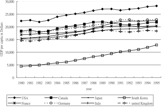
Figure 1 shows GDP per capita of eight countries, which are the only countries with complete data for GDP, GDP per capita, high-tech industries production, and all five knowledge-based service industries. It can be seen in Figure 1 that the USA has the highest GDP per capita while South Korea has the lowest.
0 5,000 10,000 15,000 20,000 25,000 30,000 1980 1981 1982 1983 1984 1985 1986 1987 1988 1989 1990 1991 1992 1993 1994 1995 year
GDP per capita in Dollars
USA Canada Japan South Korea France Germany Italy united Kingdom
Figure 1. Real GDP per capita for 8 selected countries. Data obtained from Science and Engineering Indicators, 2000, (Appendix Table 7-2), National Science Board. Virginia,
Author (http,//www.nsf-gov/sbe/srs/seind00/append/7c/at07-02.xls)
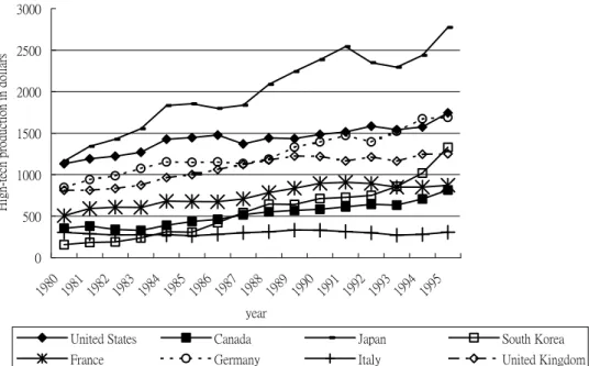
In the Figure 2 and Figure 3, however, Japan has superseded the USA as the country with the highest high-tech production per capita and highest knowledge-based service industry production per capita since 1980, but its GDP per capita has still stayed behind the USA.
0 500 1000 1500 2000 2500 3000 1980 1981 1982 1983 1984 1985 1986 1987 1988 1989 1990 1991 1992 1993 1994 1995 year
High-tech production in dollars
United States Canada Japan South Korea France Germany Italy United Kingdom
Figure 2. High-tech production per capita for 8 selected countries. Data obtained from Science and Engineering Indicators, 2000, (Appendix Table 7-1, 7-2 and 7-4), by
National Science Board. Virginia, Author.
(http,//www.nsf-gov/sbe/srs/seind00/append/7c/at07-01.xls) (http,//www.nsf-gov/sbe/srs/seind00/append/7c/at07-02.xls) (http,//www.nsf-gov/sbe/srs/seind00/append/7c/at07-04.xls) 0 2000 4000 6000 8000 10000 12000 1980 1981 1982 1983 1984 1985 1986 1987 1988 1989 1990 1991 1992 1993 1994 1995 year
Service production in dollars
USA Canada Japan South Korea France Germany Italy England
production per capita for 8 selected countries. Data obtained from Science and
Engineering Indicators, 2000, (Appendix Table 7-1, 7-2 and 7-5,), by National Science
Board. Virginia, Author (http,//www.nsf-gov/sbe/srs/seind00/append/c7/at07-01.xls) (http,//www.nsf-gov/sbe/srs/seind00/append/c7/at07-02.xls)
(http,//www.nsf-gov/sbe/srs/seind00/append/c7/at07-05.xls)
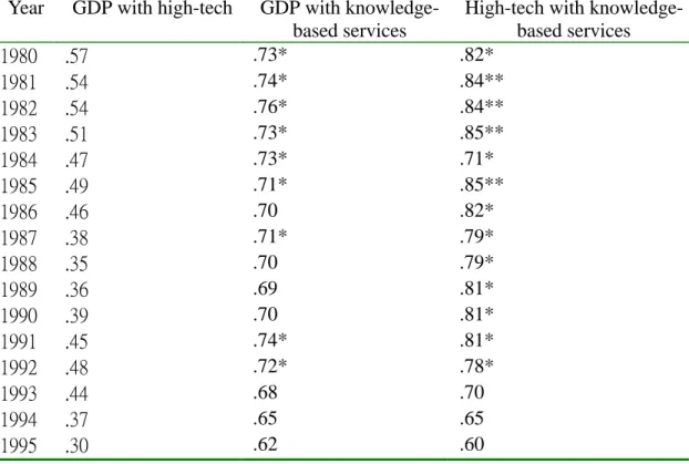
It is not easy to reach a clear understanding as one views figures which have eight curves in each. Table 1 would help us to have a better insight. If the technology gap theory is true, then the correlation between GDP and technology production variables would be significant.
Table 1 is the Pearson correlations between these three variables of the eight selected countries.
Table 1.
Pearson Correlations Between GDP Per Capita, High-Tech Production Per Capita, and All Five Knowledge-based Service Production Per Capita of the Eight Selected Countries (N= 8)
Year GDP with high-tech GDP with knowledge-based services
High-tech with knowledge-based services 1980 .57 .73* .82* 1981 .54 .74* .84** 1982 .54 .76* .84** 1983 .51 .73* .85** 1984 .47 .73* .71* 1985 .49 .71* .85** 1986 .46 .70 .82* 1987 .38 .71* .79* 1988 .35 .70 .79* 1989 .36 .69 .81* 1990 .39 .70 .81* 1991 .45 .74* .81* 1992 .48 .72* .78* 1993 .44 .68 .70 1994 .37 .65 .65 1995 .30 .62 .60 *p<.05, **p<.01
From Table 1, it can be seen that association between GDP per capita and
technology has become weaker and weaker in recent years, and all five knowledge-based service industry production per capita has a stronger correlation with the GDP per capita
than high-tech production per capita. After 1993, the correlation between technology
variables (the high-tech as well as the service industries) and GDP per capita has not been significant any more. Therefore the technology-gap theory is only partially supported.
Investigating the Potential Contribution of Education to the International Competitiveness
Among the 139 variables of hard data from the International Institute for
Management and Development (2000), 111 have significant correlations with GDP per capita (See Appendix A), but only 37 have significant correlations with GDP growth per capita (See Appendix B). The correlation between GDP per capita and GDP growth per capita is not significant (r (45) = .26).
In Table 2, the variable “R&D personnel per 1000 people” accounts for 61.66% of the total variance in the dependent variable. As the other educational variables were added to the regression equation, no increments to the R2 were observed. The matrix of
correlations in Table 3 makes clear that all the four education-related variables analyzed in Table 2 have significant correlation with GDP per capita, and they are interdependent with the exception of correlation between the “ratio of science and engineering degrees to the 24-year-old population in 1997” and the “pupil-teacher ratio in secondary education.” Consequently, the variable “R&D personnel per 1000 people” can be used as a
representative variable for education-related variables contributing to GDP per capita.
Table 2.
Coefficients From the Regression of GDP Per Capita on Education-related Variables
Model 1 Model 2 Model 3 Model 4 Model5
R&D personnel .79** .67** .54** .46* S & E degrees .62** .15 .18 .22 Enrollment .13 .07 Pupil-teacher ratio -.18 F values F (1,40)= 66.93** F (1,41)= 25.45** F (2,37)= 28.23** F (3,33)= 16.18** F (4,31)= 12.21** Adjusted R2 .6166 .3679 .5827 .5585 .5616
Notes, R&D personnel = Total R&D personnel nationwide / 1000 people;
S&E degrees = Ratio of science and engineering degrees to the 24-year-old population in 1997; Enrollment = Secondary school enrollment / Relevant age group;
Pupil-teacher ratio = Pupil-teacher ratio in secondary education
Table 3
Correlations Between Education-related Variables
1. GDP per capita (N=47) 2. Total R&D personnel nationwide /1000people (N=42) 3. Ratio of science & engineer degrees to the 24-year-old population in 1997 (N=43) 4. Secondary school enrollment/ relevant age group (N=43) 5. Pupil-teacher ratio in secondary education (N=45) 1 -- .79** .68** .63** -.45** 2 -- .70** .73** -.47** 3 -- .59** -.17 4 -- -.37* * p<.05 ** p<.01
Testing the Competitiveness Theory
We treat GDP per capita (or GDP growth per capita) as the dependent variable and choose one variable, which had the highest correlation coefficient with the dependent variable, from each factor (there being eight factors as described previously) of
competitiveness used by the IMD as the regressors in the multiple regression equation, it turns out that in Model 1 of Table 4, the adjusted R2= .9318, i.e. seven variables can explain 93.18% of variance in the GDP per capita. The negative signs of the first two variables were due the multicollinearity, because all exogenous variables had positive significant correlation with each other and with the endogenous variable. After omitting these two variables, the R2 remained almost the same (0.9316). The R2 in Model 3 with the GDP growth per capita as the dependent variable was only 0.5001. In Table 4, it was concluded that it was more difficult to predict the GDP growth per capita than to predict the GDP per capita from other Indicators of international competitiveness adopted by IMD, because the GDP growth per capita had lower and less correlations with the independent variables. Thus, the GDP per capita, instead of GDP growth per capita, was chosen as a representative variable for the product element of the international
Table 4.
Comparison of Predictability of GDP Per Capita and GDP Growth Per Capita as an Endogenous Variable.
Dependent variable = GDP per capita
Dependent variable = GDP growth per capita
Model 1 Model 2 Model 3
Direct investment stocks abroad -.08 Growth in exports of goods .22 Collected personal income tax / GDP -.02 Central government
budget surplus (or deficit) / GDP
.11
Country credit rating .2* .17* Short-term interest rate-.12
Computer power per capita .23 .23* Telephone lines / 1000 people -.34 Advertising expenditure per capita
.3** .26** Unit labor costs growth
in the manufacturing sector
.05
Total expenditure on R&D per capita
.29** .28** Total expenditure on R&D / GDP -.07 Human development index .11 .13 Secondary school enrollment / relevant age group .84**
Model 1 Model 2 Model 2
F values F (7,36) = 84.88** F (5,38) = 118.09** F (7,32) = 6.57** Adjusted R2 .9318 .9316 .5001 *p<.05 **p<.01 Table 5
Different Structural Equation Models Demonstrating Effects of Determinants of Competitiveness
Model 1 Model 2 Model 3 Model 4 Model 5
X1=RDPERSON X1=RDPERSON X1=RDPERSON X1=RDPERSON X1=RDPERSON
Y2=LIFE X2=RDEXPEND X2=RDEXPEND X2=RDEXPEND X2=RDEXPEND
Y3=GDP Y3=LIFE X3=COMPUTER X3=COMPUTER X3=COMPUTER
Y4=CONSUMPT Y4=GDP X4=HANDY X4=HANDY X4=HANDY
η2=Compet ξ1=Techinno Y6=GDP Y6=LIFE Y6=PATENT
δ1= -0.01 η2=Compet Y7=CONSUMPT Y7=GDP Y7=LIFE
ε2=0.36 δ1=.27 ξ1=Techinno Y8=CONSUMPT Y8=GDP
ε3=0.00 δ2=0.08 ξ2=Techinfr ξ1=Techinno Y9=CONSUMPT
ε4=0.05 δε23= −0.06 η3=Compet ξ2=Techinfr ξ1=Techinno
λ22=0.80* ε3=0.36 δ1=0.23 ξ3=Market ξ2=Techinfr λ32=1.00* ε4= 0.00 δ2=0.13 η4=Compet ξ3=Market λ42=0.97* ε5=0.06 δ3=0.08 δ1=.23 η4=Patents ζ2=0.40 λ11=0.85∗ δ4=0.31 δ2=.13 η5=Compet γ21=0.77∗ λ21=0.96∗ δ34=−0.03 δ3=.11 δ1=.22 λ32=0.80∗ ε5=0.32 δ4=.34 δ2=.10 λ42=1.00 ε6=0.02 δ5=0.11 δ3=.13 λ52=0.97∗ ε7=0.08 ε6=0.33 δ4=.36 ζ2=0.17 λ11=0.88∗ ε7=0.03 δ5=0.15 γ21=0.91∗ λ21=0.93∗ ε8=0.07 δ34=0.02 λ32=0.96∗ λ11=0.88∗ ε6=0.06 λ42=0.83∗ λ21=0.93∗ ε7=0.33 λ53=0.82∗ λ32=0.94∗ ε8=0.02 λ63=0.99∗ λ42=0.81∗ ε9=0.08 λ73=0.96∗ λ53=1.00 λ11=0.88∗ ζ3=0.07 λ64=0.82∗ λ21=0.95∗ φ12=0.89∗ λ74=0.99∗ λ32=0.93∗ γ31=0.21 λ84=0.97∗ λ42=0.80∗ γ32=0.78∗ ζ4=0.03 λ53=1.00 φ12=0.91∗ λ64=1.00 φ13=0.83∗ λ75=0.82∗ φ23=0.91∗ λ85=0.99∗ γ41=0.04 λ95=0.96∗ γ42=0.64 ζ4=0.26 γ43=0.33 ζ5=0.02 φ12=0.91∗ φ13=0.81∗ φ23=0.92∗ β54=0.01 γ41=0.82∗ γ52=0.55 γ53=0.47∗ χ(1,Ν=42)=0.002, p= 0.96 χ(3,Ν=42)=3.69, p= 0.30 χ(10,Ν=42)= 3.61 , p= 0.96 χ(14,Ν=42)= 4.66 , p= 0.99 χ(19,Ν=42)= 14.2 , p= 0.77
GFI=1.00 GFI=1.00 GFI=1.00 GFI=1.00 GFI=1.00
RMR= .00 RMR= .0085 RMR= .031 RMR= .028 RMR= .026
R2= .60 R2= .830 R2= .93 R2= .97 R2= .98
Note.
RDPERSON= Total R&D personnel nationwide / 1000people RDEXPEND= Total expenditure on R&D per capita
HANDY= Cellular mobile telephone subscribers / 1000 people
ADVERTIS= Advertising expenditure per capita
PATENT= Number of patents in force / 100000 inhabitants LIFE= Life expectancy at birth. GDP= GDP per capita CONSUMPT= Private consumption expenditure per capita
Techinno= Technology innovation activities Techinfr=Technological infrastructure Market=Market activity Patents=Granted Patents Compet=Competitiveness * At least significant at .05 level
ζ4=.28 δ1=.22 . λ64=1.00 ε6=.06 λ11=.88∗ λ21=.95* γ41=.82* γ54 =.02 ε7=.33 δ2=.10 λ75=.82* δ3=.13 γ52=.55 λ85=.99* ε8=.02 λ32=.93∗ λ95=.96* δ34=.02 ζ5=.02 ε9=.08 γ53=.47* δ4=.36 λ42=.80* δ5=.15 λ53=1.00
Figure4. Effect of patents, high-tech infrastructure and market activity on the competitiveness
with patents in force per 100000 habitants as intervening variable. * At least significant at .05 level
Table 5 demonstrates different models of LISREL. Because of multicollinearity, it is necessary to introduce variables step by step to show the effect of education on the competitiveness.
The parameter specifications used by Jöreskog & Sörbom (1993) were applied, but with miner amendment in the present study. Instead of (X)
IJ
λ and (Y)
IJ
λ , λij was
employed to stand for the standardized effect of a latent variable on an observed variable. X1=R&D personnel X2=R&D expenditure Y9=Consu mption per capita Y8=GDP per capita Y7=Life expectancy ξ1=Innov ation η5= Comp etitive ness ξ2= Hi-tech infrastr ucture X3=Compute rs per 1000 people X4=Mobile telephone per 1000 people ξ 3=Market activity X5=Adve rtising per capita η4=Pat ents Y6=Pate nts in force / 100000 people
Therefore, the serial number of the first latent endogenous variable follows that of the last
latent exogenous variable, and the serial number of the first observed endogenous variable comes after that of the last observed exogenous variable.
The international competitiveness is a latent variable (an abstract construct) and must be indicated by measurable and observable variables. It was indicated by three observed variables: life expectancy at birth, GDP per capita, and private consumption expenditure per capita.
In the Model 1 of Table 5, “R&D personnel per 1000 people” was selected as an indicator for human capital produced by education. γ21=0.77* in Model 1 means that the
education makes a significant contribution to competitiveness. Adjusted R2= .60
designates that education alone can explain 60% of the variance in competitiveness. This result supports the second hypothesis that the education-related variable “R&D personnel per 1000 people” does have a significant association with the competitiveness-related variables.
In Model 2, “total expenditure on R&D per capita” was combined with “R&D personnel per 1000 people” to form indicators for the latent variable “technological innovative activities”. The latent variable “innovative activities ”explained 83% of variance in competitiveness, γ21=0.91* denoting that “innovative activities” is a
significant determinant of competitiveness. The error term δε23=-0.06 was generated
by a statement: “set the errors between RDEXPEND and LIFE correlate” in the LISREL 8 program, because the Maximum Modification Index located at this term. After
modification, the fitness of the model improved.
In Model 3 and Model 4, the latent variables “technological infrastructure” and “market activity” were introduced stepwise. They both brought about increment of R2.
“Granted patents” was inserted to Model 5 as an intervening variable between
innovative activity and competitiveness. The diagram of Model 5 is presented in Figure 4. The non-significance of γ31 (the effect of innovative activities on competitiveness) in
Model 3 was due to multicollinearity, because it was originally significant in Model 1. Its effect was partialed out. γ41、γ42、γ43 in model 4 and γ52 in Model 5 are much the same.
4.The case of Taiwan
The situation of Taiwan is analogous to that of Switzerland. They are small countries with scarce resources and limited domestic market. Their competitiveness hangs on human capital, especially on the innovation of R&D personnel. To cultivate more and more creative R&D personnel is what the education can contribute to competitiveness. In this case, Switzerland is a model country for Taiwan. From Table 6, it can be seen that R&D personnel per 1000 people in Switzerland is about 1.5 times as many as in Taiwan. To catch-up the level of Switzerland in this respect would be a reasonable goal for the educational policy of Taiwan, if Taiwan wants to improve its international
Table 6
Different structural equation models demonstrating effect of determinants of competitiveness Code number of IMD Variable Value of Taiwan Rank of Taiwan Value of Switzerland Rank of Switze rland Value of best country 1.02 GDP per capita $13,111 25 $36,071 2 $44424(Luxemb ourg) 1.14 Private consumption expenditure per capita $7,973 26 $18,260 5 $21953(USA) 5.12 Number of computers/100 0 people 260.1 23 408.3 10 538.9(USA) 5.18 Cellular mobile telephone subscribers/ 1000 people 493.60 10 441.65 13 679.10(Finland) 6.18 Advertising expenditure per capita 151.1 19 346.53 13 419.41(USA) 7.02 Total expenditure on R&D per capita $242.80 20 1142.3 1 1143.2(Switzerla nd) 7.07 Total R&D personnel /1000people 4.662/1000 people 14 7.11 2 7.401(Sweden) 7.26 Number of patents in force/100000 in habitants 686.8/1000 00 people 7 1342.2 1 1342.2(Switzerla nd) 8.05 Life expectancy at birth 73.7 31 79.1 5 80.3(JAPAN)
Discussion
Analyzing longitudinal and cross-sectional data from the data base of American National Science Board (2000) and the International Institute for Management and Development (2000), the present study found that: (a) ”knowledge-based service industry production per capita” has a stronger correlation with the GDP per capita than high-tech production per capita does, (b) the technology gap theory assuming that if the countries falling behind want to reach the level of economic growth of countries with a higher GDP per capita, a promising way is to commit themselves to technological catch-up (Dosi, et al, 1990; Fagerberg, 1994) was only partially supported, as Japan has taken the place of the USA as the country with the highest high-tech production per capita and highest knowledge-base service industry production per capita since 1980, but the GDP per capita has still stayed behind the USA ever since, (c) Among education-related variables, which may contribute to competitiveness, “R&D personnel per 1000 people” is most suitable choice as indicator for the latent variable “education,” because it has stronger correlation with GDP per capita than other variables , such as “ratio of science and engineer degrees to the 24-year-old population,” “ratio of secondary school enrollment to the relevant age group,” or “pupil-teacher ratio in secondary education,” (d) ”R&D personnel per 1000 people” standing alone, can explain 60% of variance in
competitiveness, which was represented by three observed variables: “life expectancy at birth,” “GDP per capita,” and “private consumption expenditure per capita.”
The significant correlation between the “ratio of secondary school enrollment to the relevant age group” and GDP per capita found in the present study confirms the result of Mankiw, Romer, & Weil’s (1992) study which demonstrated that adding human capital, with the “ratio of secondary school enrollment to the relevant age group” as a proxy, to the exogenous variables (saving and population growth) of regression equation led to a significant increment of .2 in R2.
The result of the present study seems to discount the assertion that a technology gap is the only cause for the differences in GDP per capita across counties, but technological innovation remains to a substantial factor in influencing international competitiveness. Perhaps GDP per capita could also be influenced by other variables, such as labor costs and forms of industrial organization, as proposed by Dosi, et al. (1990, p.160).
The results displayed in Figure 1 to Figure 3 are constructed with sample data from only eight developed and newly industrializing countries, so that they can not be generalized to the developing countries. Further researches in this respect are needed.
A direct way to expand the number of R&D personnel is to increase the scale of doctoral programs in Science and Engineering. The National Science Board ( 2000, Chapter 4 ) describes the worldwide effort to expand doctoral programs in science and engineering. The major Asian countries, China, India, Japan, South Korea, and Taiwan, awarded science and engineering degrees in an average annual increment of 12% from 1993 to 1997. In Germany, the number of science and engineering degrees increased 4.3% annually between 1975 and 1997, but non-science and engineering doctoral degrees increased only 2.8% during this period. The number of science and engineering doctoral degrees awarded in France from 1989 to 1997 increased about 83%.
All the endeavors of strengthening and expanding doctoral education in science and engineering are to develop the capacity for high quality research leading to technological
innovation and to build up the knowledge-based economy, and in the end to gain strength
in competitiveness.
References
Boltho, A. (1996). The assessment of international competitiveness. Oxford Review of Economic Policy, 12 (3), 1-16.
Dosi, G. (1988). Sources, procedures, and microeconomic effects of innovation. Journal of Economic Literature, 26, 1120-1171.
Dosi, G, Keith, K. and Soete, L. (1990). The economics of technical change and international trade. London: Harvester Wheatsheaf.
Fagerberg, J. (1988). International competitiveness. The Economic Journal, 98, 355-374.
Fagerberg, J. (1994). Technology and international differences in growth rates. Journal of Economic Literature, 32, 1147-1175.
Fagerberg, J. (1996). Technology and competitiveness. Oxford Review of Economic Policy, 12 (3), 39-51.
International Institute for Management and Development. (2000). The world competitiveness yearbook 2000. Lausanne, Switzerland: Author.
Jöreskog, K. & Sörbom, D. (1993). Structural equation modeling with the SIMPLIS command language (LISREL 8). Hillsdale, NJ:Lawrence Erlbaum Associates
Publishers.
Llewellyn, J. (1996). Tackling Europe’s competitiveness. Oxford Review of Economic Policy, 12 (3), 87-96.
Mankiw, N. G., Romer, D., & Weil, D. N. (1992). A contribution to the empirics of economic growth. The Quarterly Journal of Economics , May, 407-437.
National Science Board. (2000). Science and Engineering Indicators, 2000. Virginia:
Author. Available online, http,//www.nsf-gov/sbe/srs/seind00/ (downloaded May 2001).
Organization for Economic Cooperation and Development. (1992). Technology and the economy: The key relationships. Paris: Author.
Scott, A. J. & Storper, M. (1987). High technology industry and regional development: A theoretical critique and reconstruction. International Social Science Journal, 112,
215-232.
Windrum, P. & Tomlinson, M. (1999). Knowledge-intensive services and international competitiveness, A four-country comparison. Technology Analysis & Strategic Management, 11 (3), 391-405.
APPENDIX A
Variables, which have significant correlation coefficient with GDP per capita
Code of
IMD Variables r
1.01 GDP .33*
1.04 GDP per capita estimates .97**
1.07 Gross national income .33*
1.10 Total gross domestic investment .32*
1.13 Gross domestic savings real growth .37*
1.14 Private consumption expenditure per capita .97** 1.16 Government final consumption expenditure .37**
1.19 Non-agriculture economic sector/ GDP .62**
1.23 Retail sales .95**
1.24 Real growth in retail sales .51**
1.25 Annual rate of consumer price inflation .37*
1.26 Cost-of-living comparisons .59**
2.04 Balance of commercial services/GDP .30*
2.07 Exports of goods .39**
2.08 Exports of goods/GDP .39**
2.10 Exports of commercial services .41**
2.11 Experts of commercial services/GDP .39**
2.17 Imports of goods and commercial services .38** 2.19 Growth in imports of goods and commercial services .33*
2.25 Portfolio investment assets .47**
2.26 Portfolio investment liabilities .40**
2.27 Direct investment flows abroad .42**
2.28 Direct investment stocks abroad .52**
2.31 Direct investment stocks inward .32*
3.01 Central government domestic debt .41**
3.06 Central government budget surplus/deficit GDP .57**
3.10 General government expenditure/GDP .51**
3.12 Collected total tax revenues/GDP .55**
3.13 Effective personal income tax rate/GDP per capita .43**
3.14 Collected personal income tax/ GDP .62**
3.16 Collected employee's social security contribution/GDP .36* 3.23 Collected capital and property taxes/ GDP .61**
4.03 Country credit rating .85**
4.09 Factoring (% of merchandise exports) .38**
4.12 Stock market capitalization .32*
4.13 Value traded on stock markets per capita .49** 4.18 Number of banks among world's top 500 (ranked by assets) .38**
4.19 Banking sector assets .45**
4.26 Number of credit cards issued .59**
4.27 Credit card transactions .65**
5.03 Roads(density of network) .43**
5.04 Railroad (density of network) .40**
5.10 Investment in telecommunications(95-97) -.43** 5.11 Computers in use(% of worldwide computer in use) .34*
5.12 Number of computers/1000 people .88**
5.13 Computer power .34*
5.14 Computer power per capita .92**
5.15 Connections to internet/1000 people .67**
5.18 Cellular mobile telephone subscribers/ 1000 people .77**
5.19 Office rent .31*
5.21 Telephone lines/ 1000 people .90**
5.23 Total health expenditure/GDP .67**
5.24 Public expenditure on health/GDP .38*
5.25 Number of doctors per 10000 inhabitants .40**
5.28 Commercial energy consumed/GDP -.53**
5.33 % of population served by waste water treatment plants .58** 5.34 GDP/per metric tons of CO2 emission =co2 control -.60**
6.01 Estimated GDP per employee .87**
6.02 GDP per employee .97**
6.04 GDP (PPB) estimates per employee per hour .88**
6.05 GDP per employee per hour .97**
6.06 Estimated GDP per employee in agriculture .57**
6.07 GDP per employee in agriculture .71**
6.08 Estimates GDP per employee in industry .72**
6.09 GDP per employee in industry .90**
6.10 Estimates GDP per employee in service .80**
6.11 GDP per employee in services .95**
6.13 Unit (labor costs growth in the manufacturing sector) -.30*
6.14 Remuneration of primary school teacher .81**
6.15 Remuneration of engineer .68**
6.16 Number of companies in fortune 500 companies (ranked by sales) .38**
6.18 Advertising expenditure per capita .90**
7.01 Total expenditure on R&D .41**
7.02 Total expenditure on R&D per capita .88**
7.03 Total expenditure on R&D /GDP .74**
7.04 Business expenditure on R&D .40**
7.05 Business expenditure on R&D per capita .82** 7.07 Total R&D personnel nationwide /1000people .79** 7.09 R&D personnel in business per capita .76**
7.17 Nobel prizes since 1950 .29*
7.18 Nobel prizes per capita .56**
7.22 Patents granted to residents .32*
7.24 Securing patents abroad .45**
7.26 Number of patents in force/100000 inhabitants .74**
8.01 Estimates of population -.29*
8.02 % of population under 15 years -.67**
8.03 % of population over 65 years .70**
8.04
Dependency ratio population under 15 and over 64 years / active
population (15-64years) -.38**
8.05 Life expectancy at birth .78**
8.07 Labor force / population .42**
8.09 Active population (15-64years)total population .37* 8.14 % of employment by non-agriculture sector .67**
8.16 Employment/population .51**
8.19 Number of working hours per year -.59**
8.20 Unemployment/work force -.33*
8.21 Unemployment of population under 24years/ total unemployment -.45** 8.23 Secondary school enrollment/ relevant age group .63** 8.27 Pupil-teacher ratio in primary education -.50** 8.28 Pupil-teacher ratio in secondary education -.45** 8.29 Total and current public expenditure on education/ GNP .34* 8.30 Non-illiteracy adult (over 15 years) literacy / population .52**
8.33 Urban population/ total population .32*
8.34 Income distribution lowest 20% .38**
8.35 Income distribution highest 20% -.58**
8.38 Human development index .82**
Ratio of science & engineer degrees to the 24-year-old population
in 1997 .62**
*p<.05 **p<.01
APPENDIX B
Variables, which have significant correlation coefficient with real GDP growth per capita
Code of
IMD Variables r
1.04 GDP per capita estimates .30*
1.05 Real GDP growth .96**
1.12 Growth domestic savings/GDP .34*
1.13 Gross domestic savings real growth .46** 1.15 Growth in private final consumption expenditure .31*
2.09 Growth in exports of goods .42**
2.18 Imports of goods and commercial services/GDP .30*
2.23 Exchange rate stability -.42**
2.43 (Exports + Imports)/GDP*2 .31*
3.06 Central government budget surplus (or deficit)/GDP .44** 3.09 Government employment/ total employment .32*
3.12 Total tax revenues/ GDP .29*
3.23 Collected capital and property taxes/ GDP .39**
4.01 Short-term interest rate -.47**
4.03 Country credit rating .39**
5.12 Number of computers/1000 people .32*
5.14 Computer power per capita .31*
5.21 Telephone lines/ 1000 people .33*
6.01 Estimated GDP per employee .31*
6.03 GDP growth per person employed .79** 6.04 GDP (PPB) estimates per employee per hour .29* 6.10 Estimates GDP per employee in service .34* 6.13 Unit labor costs growth in the manufacturing sector -.49** 7.03 Total expenditure on R&D /GDP .33*
8.02 % of population under 15 years -.44**
8.04
Dependency ratio population under 15 and over 64
years / active population (15-64years) -.48**
8.07 Labor force / population .40**
8.11 Female labor force/ total labor force .45**
8.16 Employment/population .43**
8.19 Number of working hours per year -.31*
8.20 Unemployment/work force -.31*
8.23 Secondary school enrollment/ relevant age group .64** 8.26math TIMSS average achievement of 8th grade .38* 8.26scie TIMSS average achievement of 8th grade .44* 8.35 Income distribution highest 20% -.54** *p<.05 **p<.01