利用GARCH-NIG Model對台指選擇權定價

國

立

交

通

大

學

統計學研究所

碩

士

論

文

利用 GARCH-NIG Model 對台指選擇權定價

Pricing the TAIEX option with GARCH-NIG Model

研 究 生：葉宇青

指導教授：李昭勝 教授

利用 GARCH-NIG Model 對台指選擇權定價

Pricing the TAIEX option with GARCH-NIG Model

研 究 生：葉宇青 Student：Yu -Ching Yeh

指導教授：李昭勝 Advisor：Dr. Jack C. Lee

國 立 交 通 大 學 統計學研究所

碩 士 論 文

A Thesis

Submitted to Institute of Statistics College of Science

National Chiao Tung University in Partial Fulfillment of the Requirements

for the Degree of Master

in Statistics June 2004

Hsinchu, Taiwan, Republic of China

誌 謝

即將揮別研究所的生涯，在這期間能夠完成我的碩士論文，除了 增加對自我能力的肯定之外，也讓更融會貫通將書本上的知識來應用 在這篇論文上。在這之中，首要感謝的是我的指導老師李昭勝教授細 心、以及專業的指導，讓我在這一路上更有信心來往前邁進，再來是 博士班的學長牛維方耐心不厭其煩的指導我，讓論文可以順利完成， 在這背後，我的父母給我精神上的支柱也是一大力量。 接下來要感謝的我研究所的同學，陪我在唸書之餘打球來娛樂身 心，也適時的在我需要幫助的時候給我鼓勵以及幫助，讓我可以完成 碩士論文。最後我把我的碩士論文送給大家，與每個人分享我的榮 耀，謝謝你們。 葉宇青 謹誌于 國立交通大學統計學研究所 中華民國九十三年六月

利用 GARCH-NIG Model 對台指選擇權定價

研究生：葉宇青 指導教授：李昭勝 博士

國立交通大學統計學研究所

摘 要

此 篇 論 文 的 重 點 在 於 對 台 指 的 選 擇 權 來 做 評 價 ， 利 用 Barndorff-Nielsen 在 1997 年提出的 Normal Inverse Gaussian 的 分配再加上變異數服從 GARCH 的過程形成 GARCH-NIG 的模型。

利用最大概似估計法來估計模型中之參數，再利用 Monte Carlo 的方法來預測選擇權價格。接著與 Black-Schole 模型預測出的價格 做比較。

Pricing the TAIEX option with GARCH-NIG Model

Student：Yu -Ching Yeh Advisors：Dr. Jack C. Lee

Institute of Statistics

National Chiao Tung University

ABSTRACT

In this paper，we focus on pricing option of TAIEX using GARCH-NIG model

formed by Normal Inverse Gaussian(NIG) distribution proposed by Barndorff-Nielsen

in 1997 combined with the variance of NIG distribution following GARCH process.

Using maximum likelihood estimation method to estimate parameters within

model . After that, we forecast option price using Monte Carlo method and compare

Table of Contents

Acknowledgements i

Chinese Abstract ii

English Abstract iii

Table of contents iv

Introduction 1

1. The model 5

1.1 Normal Inverse Gaussian distribution 5

1.2 The GARCH-NIG option pricing model 7

2. Estimation of the model 10

3. Empirical analysis 11

3.1 Market description 11

3.2 Description of data 14

3.3 Comparison with other option pricing models 17

4. Numerical results and discussion 18

5. Conclusions 23

6. Appendices 24

7. R e f e r e n c e s 2 6

Introduction:

Numerous recent studies on option pricing have acknowledged the fact that volatility changes overtime in time series of asset returns as well as in the empirical variances implied from option prices through the Black & Scholes (1973) model. Many of these studies focused on modeling the asset return dynamics through stochastic volatility (SV) models. Due to analytically intractable likelihood functions and hence the lack of available efficient estimation procedures, SV models were until recently viewed as an unattractive class of stochastic process compared to other time-varying volatility processes, such as ARCH/GARCH models. Moreover, to calculate option prices based on SV models we need, besides parameter estimates, a representation of the unobserved historical volatility, which is again far from being straightforward to obtain. Therefore, while the SV generalization of option pricing has, thanks to advances in econometric estimation techniques, recently been shown to improve over the Black-Scholes model in terms of the explanatory power for asset-return dynamics, its empirical implications on option pricing itself have not yet been adequately tested due to the aforementioned lack of a representation of the unobserved volatility. Can the SV generalization of the option pricing model help resolve the well-known systematic empirical biases associated with the Black-Scholes model, such as the volatility “smile” (e.g. Rubinstein (1985)), asymmetry of such “smile” or “smirk” (e.g. Stein (1989))? How substantial is the gain, if any, from such generalization compared to relatively simpler models? The purpose of this thesis is to answer the above questions by studying the empirical performance of SV models in pricing options on the TAIEX, and investigating the respective effect of stochastic interest rates, stochastic volatility, and asymmetric asset returns on option prices

in a multivariate SV model framework.

The NIG (Normal Inverse Gaussian) distribution is well-known in financial field. So, in this thesis we use NIG model to model returns. Using daily data from Taiwan’s market, we would like to show that NIG model is a good model for stock returns compared with other option pricing models. For more details about Normal Inverse Gaussian (NIG), see Barndorff-Nielsen (1997).

The seminal ARCH paper by Engle (1982) triggered one of the most active and fruitful areas of research in econometrics over the past two decades. The success of the ARCH/GARCH class of models at capturing volatility clustering in financial markets is well documented (see, for example, Bollerslev, Chou and Kroner, 1992). Meanwhile, the inability of the ARCH/GARCH models coupled with the auxiliary assumption of conditionally normally distributed errors to fully account for all of the mass in the tails of the distributions of say, daily returns, is also well recognized. Indeed, several alternative error distributions were proposed in the early ARCH literature to better account for the deviation from the normality in the conditional distributions of the returns, including the t-distribution of Bollerslev (1987), the General Error Distribution (GED) of Nelson (1991), and more recently, the Normal Inverse Gaussian (NIG) distribution of Barndorff - Nielsen (1997), Anderson (2001) and Jensen and Lunde (2001). The motivation behind these alternative error distributions has been almost exclusively empirical and pragmatic in nature. In the present thesis, building on the Mixture of Distribution Hypothesis (MDH) (Clark, 1973) along with the recent idea of realized volatility (RV), we provide a sound empirical foundation for the distributional assumptions underlying the GARCH-NIG model.

Be consistent with the absence of arbitrage and a time-changing Brownian motion, the MDH postulates that the distribution of returns is normal, but with a stochastic variance. In the original formulation in Clark (1973), the variance is assumed to be i.i.d. lognormally distributed, resulting in a lognormal-normal mixture distribution for the returns. Importantly, to explicitly account for the volatility clustering effect Taylor(1982, 1986)proposed an extension of the MDH setup by making the latent logarithmic variance to follow a Gaussian autoregression, resulting in the lognormal Stochastic Volatility(SV) model; see also Anderson(1996). Since the joint distribution of the returns in the SV model is not known in closed form, both estimation and inference for these types of models are considerably more complicated than for the ARCH/GARCH class of models.

In contrast to the existing SV literature, which treats the mixing variable as latent, we have shown that by measuring the daily variance by the corresponding realized volatility constructed from the sum of intraday high-frequency returns, the daily return standardized by the realized volatility is approximately normally distributed. Therefore, even though the realized volatilities are subject to measurement error vis-à-vis the true daily latent volatilities, the normality of the standardized returns is consistent with the basic tenets of the MDH and the use of the realized volatility as the underlying mixing variable. Moreover, we find that the distribution of the realized volatility conditional on the past squared daily returns (as well as the unconditional distribution of the realized volatility) is closely approximated by an Inverse Gaussian (IG) distribution. Taken together, these results imply that in practical modeling situations where the high-frequency data are not actually available, the daily returns should be well described by a NIG model.

GARCH-NIG option pricing model. In section 2, we introduce the method to estimate parameters in GARCH-NIG option pricing model. In section 3, we describe empirical analysis, including market description and data description. Section 4 presents the results and some discussions. Section 5 concludes.

1. The Model

1.1 Normal Inverse Gaussian distribution

The Mixture-of-Distributions Hypothesis (MDH) starts from the premise that the distribution of discretely sampled returns, conditional on some latent information arrival process, is Gaussian. This assumption is justified theoretically if the underlying price process follows continuous sample path diffusion (see, for instance, the discussion in Andersen et al., 2002, and Barndorff- Nielsen and Shephard, 2001). However, the integrated volatility process that serves as the mixture variable in this situation is not directly observable. As noted above, this has spurred numerous empirical investigations into the use of alternative volatility proxies and/or mixture variables. Meanwhile, in the diffusion setting the integrated volatility may, in theory, be estimated arbitrarily well by the summation of finely sampled squared high-frequency returns, or so-called realized volatilities. This suggests the following empirically testable starting point for the MDH,

) , 0 ( ~ | t t t RV N RV r , ₍₁₎

where refers to the discretely sampled one-period returns from time t -1 to t,

and denotes the corresponding realized volatility proxy measured over the

same time interval.

t r t RV (2) ) , ( ~ IG h

α

RV_t ,

where the density function for the IG distribution may be expressed in standardized form as,

)} ) ( ) ( ( 2 1 exp{ ) 2 ( ) ( ) 1 ( ) , ; ( 2 1 2 3 2 1 h RV RV h RV h h RV IG t t t t

α

α

α

π

α

α

= − + − − , ₍₃₎

Now, combining the distributional assumptions in (1) and (2) the implied unconditional distribution for the returns should be Normal Inverse Gaussian (NIG), ) , 0 , 0 , ( ) ( ) | ( ) ( 0

α

h NIG dRV RV f RV r f r f _t =

∫

_{t t t t} = ∞ , ₍₄₎

with the following closed-form density function,

)) ) ( ( ( ) ) ( ( ) exp( ) , 0 , 0 , ; ( 2 1 1 1 2 1 2 1 2 1

α

α

α

α

π

α

α

h z q K h z q h h z NIG = − , where 2 1 ) (x x

q = + and denotes the modified Bessel function of

third kind and order one. The NIG distribution was first used for modeling speculative returns in Barndorff-Nielsen (1997). It may be viewed as a special case of the Generalized Hyperbolic Distribution in Barndorff- Nielsen (1978).

) ( 1 z

K

Although the NIG distribution in equation (3) may adequately capture the fat-tailed unconditional return distributions, it does not account for the well-documented volatility clustering, or ARCH, effects. In order to incorporate conditional heteroscedasticity in the return process within the MDH framework,

define theI_t−1 information set generated by the past daily returns,

...} , , { _{1 2} 1 − − − = t t t h r r I , ) , ( ) | (RV_t I_{t 1} IG h_t α f ₋ = ,

for the results reported below, the conditional mean in the IG distribution is assumed to follow the recursive GARCH(1,1) like structure,

1 1 2 1 1 0 + − + − = _{t t} t r h h

α

α

β

. ₍₅₎

The GARCH(1,1)-NIG model now arises naturally by combining equation (1)

augmented with the information set, with the

conditional distribution for in equations (4) and (5),

1 − t I rt |RVt,It−1 ~N(0,RVt−1) t RV ) , 0 , 0 , ( ) | ( ) , | ( ) | ( 0 1 1 1 t t t t t t t

α

t t I f r RV I f RV I dRV NIG h r f =

∫

= ∞ − − −

.

(6)

1.2 The GARCH-NIG option pricing model

Consider a discrete-time economy and let be the asset price at time t.

Its one-period log rate of return is assumed to be conditionally normal inverse Gaussian distributed under probability measure P. That is,

t X t t t t t h h r X X

_λ

_ε

+ − + = − 2 1 ln 1 , ₍₇₎

where ε_t has mean zero and conditional variance under measure P; r is

the constant one-period risk-free rate of return and

t h

λ

the constant unit risk

premium. We further assume that ε_t follows a GARCH (1,1) process of

Bollerslev (1986) under measure P. Formally,ε_t |φ_t−1 ~ NIG(α,0,0,h_t) under

measure P, 1 1 2 1 1 0 + − + − = _{t t} t h h

α

α

ε

β

₍₈₎

where φ_t is the information set of all information up to and including time;

0 , 0 , 0 ; 1 0 1 1 1 1 + β < α ≥ α ≥ β ≥

a linear function of the past squared disturbances and the past conditional variances.

Definition : A pricing measure Q is said to satisfy the locally risk-neutral valuation

relationship(LRNVR) if measure is mutually absolute continuous with respect to

measure P, ln( | ₁) 1 − − t t t X X

_φ

follows Normal Inverse Gaussian distribution(under Q), r t t t Q e X X E ₋ = − | ) ( 1 1

φ

where r stands for interest rate, and, ) | ) (ln( ) | ) (ln( 1 1 1 1 − − − − = _t t t p t t t Q X X Var X X Var

φ

φ

almost surely with respect to measure P.

Theorem: The LRNVR implies that, under pricing measure Q, t t t t h r X X _{= − +}

_ξ

− 2 1 ) ln( 1 , where ) , 0 , 0 , ( ~ | t 1 t t φ NIG α h ξ ₋ and 1 1 2 1 1 1 0 + ( − − − ) + − = _{t t t} t h h h

α

α

ξ

λ

β

.

Pricing contingent payoff s requires temporally aggregating one-period asset returns to arrive at a random terminal asset price at some future point in time. The terminal asset price is derived in the following corollary:

Corollary: ⎥⎦ ⎤ ⎢⎣ ⎡ _{− − +} =

∑

∑

+ = + = T t s s T t s s t T X T t r h X 1 1 2 1 ) ( exp

ξ

From above corollary, we get the following time-t value of the European call option with exercise price k maturing at time T,

] | ) 0 , [max( ) ( t T Q r t T k X E e C = − − −

φ

.

2. Estimation of the model

Estimation of the parameters of the different models is straightforward using the maximum likelihood method. The log likelihood of the sample for the GARCH-NIG models is given by

∑

∑

∑

∑

= = = = − − − − + + + = n i t i n i n i t i t n i t h X K h X h h l 1 2 1 2 1 1 1 2 1 ) ) 1 ( ( ln ) 1 ln( 2 1 ) ln 2 1 ( ) ln ln 2 1 ( ) , (

α

α

α

α

π

α

α

3. Empirical analysis

The empirical analysis starts with a description of the options data. It proceeds to estimate the GARCH-NIG model with time series data on index returns and with options data.

3.1 Market description

TSEC, Taiwan Stock Exchange Corporation, maintains stock price indices, to allow investors to grab both overall market movement and different industrial sectors' performances conveniently. The indices may be grouped into market value indices and price average indices. The former are similar to the Standard & Poor's Index, weighted by the number of outstanding shares, and the latter are similar to the Dow Jones Industrial Average and the Nikkei Stock Average. The Taiwan Stock Exchange Capitalization Weighted Stock Index ("TAIEX") is the most widely quoted of all TSEC indices. The base year value as of 1966 was set at 100. TAIEX is adjusted in the event of new listing, de-listing and new shares offering to offset the influence on TAIEX owing to non-trading activities. We summarize other details and rule of TAIEX and TXO into the following table.

Table 3.1.1

Item Description

Underlying Index

Taiwan Stock Exchange Capitalization Weighted

Stock Index (TAIEX)

Ticker Symbol TXO

Multiplier NT$ 50 (per index point)

Expiration Months

Spot month, the next two calendar months followed

by two additional months from the March quarterly

Cycle (March, June, September, and December)

Strike Price

Interval

100 index points in spot month, the next two

calendar months

200 index points in the additional two months from

the March quarterly Cycle

Strike (Exercise)

Price

When listing series of new expiration months, one

series with at-the-money strike price is listed based

on the previous day's closing price of the underlying

index rounded down to the nearest multiples of 100.

1. For the spot month and the next two calendar

months: fifth other series each with in-the-money

and out-of-the-money strike prices with price

interval of 100 points are listed.

2. For the next two quarter-months: Three other

series each with in-the-money and

out-of-the-money strike prices with price interval of

200 points are listed.

Up to the 5th business days before expiration,

1. For the spot month, and the next two calendar

months: additional series are added when the

lowest strike price available, to maintain at least 5

in- and 5 out-of-the-money strike prices

2. For the next two quarter-months: additional series

are added when the underlying trades through

the third highest or lowest strike price available,

to maintain at least3 in-and 3 out-of-the-money

strike prices

Premium

Quotation

< 10 points: 0.1 point (NT$5)

>=10 points,<50 points: 0.5 point (NT$ 25)

>=50 points, <500 points: 1 point (NT$ 50)

>=500 points, <1,000 points: 5 point (NT$ 250)

>=1,000 points: 10 point (NT$ 500)

Daily Price Limit

+/- 7% of previous day's closing price of the

underlying index

Position Limit

Individuals: 8,000contracts on either side of the

market.

Institutional Investors: 16,000 contracts on either

side of the market.

Institutional investors may apply for an exemption

from the above limit on trading accounts for hedging

purpose.

Exemptions are allowed for Future Proprietary

Trading Hours

08:45AM - 1:45 PM Taiwan time Monday through

Friday of the regular Taiwan Stock Exchange

business days

Last Trading Day The third Wednesday of the delivery month

Expiration Date The first business day following the last trading day

Final Settlement

Price

The final settlement price for each contract is

computed from the first fifteen-minute

volume-weighted average of each component

stock's prices in that index on the final settlement

day. For those component stocks that are not traded

during the beginning fifteen-minute interval on the

final settlement day, their last closing prices would

be applied instead

Settlement

Cash settlement. An option that is in-the-money and

has not been liquidated or exercised on the

expiration day shall, in the absence of contrary

instructions delivered to the Exchange by the

Clearing Member representing the option buyer, be

exercised automatically

3.2 Description of data

We use daily data on TAIEX from January 1 ,2002 to March 20, 2003 to estimate GARCH-NIG parameters. Then we use GARCH (1,1)-NIG option pricing model to forecast option price form March 21 to April 10. Each day, we chose

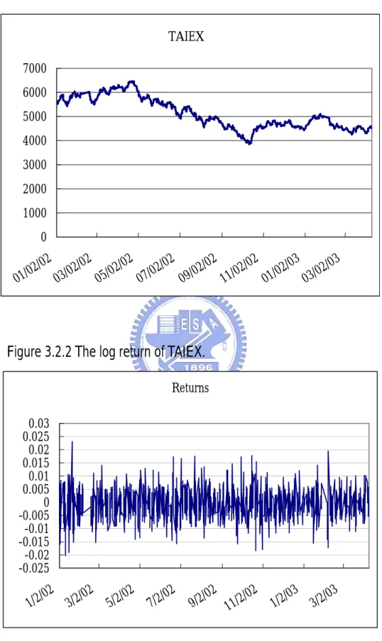
different strike prices from 4000 to 5100 and select one contract with the highest volume of trade for each strike price on that day to do call option pricing. We exclude the option data from 9:00 to 9:30 and the data after 13:25, as well. Moreover, we eliminate all transactions taking place during the last week before expiration (to avoid the expiration-related price effects). We summarize all the data we chose into the following table, respectively. The patterns of TAIEX and returns are shown in Figures 3.2.1 and 3.2.2 and results of estimation are given in Table 3.2.1.

Table 3.2.1. Estimation results. ^

0

α

α

^₁

β

^₁ ^

α

λ

^

Loglikelihood

0.0000005 0.017708 0.96425 6.0901 0.2085 3750.09

Table 3.2.2. Data summaries. Moneyness (K/S) Average price Std Number of observations In the money <0.95 372.59 96.92 29 At the money 0.95~1.05 121.28 63.15 57

Out of the money >1.05 18.33 13.38 46

Figure 3.2.1 The price pattern of TAIEX. TAIEX 0 1000 2000 3000 4000 5000 6000 7000 01/02 /02 03/02 /02 05/02 /02 07/02 /02 09/02 /02 11/02 /02 01/02 /03 03/02 /03

Figure 3.2.2 The log return of TAIEX. Returns -0.025-0.02 -0.015 -0.01 -0.005 0 0.005 0.01 0.015 0.02 0.0250.03 1/2/02 3/2/02 5/2/02 7/2/02 9/2/02 ₁₁/2/02 1/2/03 3/2/03

3.3 Comparison with other option pricing models

In this subsection, we compare the Black-Scholes with GARCH (1,1)-NIG option pricing model. Since the GARCH (1, 1) model is the most commonly used GARCH process, our discussion for the reminder of this thesis will be restricted to the GARCH (1,1)-NIG model. We have introduced GARCH (1,1)-NIG option pricing model, so now we review Black-Scholes option pricing models.

The Black-Scholes option pricing model is presented as follows. The call option price formula can be written as,

) ( ) (d₁ ke ( )N d₂ N X c = _t − −r T−t , where ) ( ) )( 2 ( ) ln( 2 1 t T t T r k X d t − − + + =

σ

σ

, ( ) ) ( ) )( 2 ( ) ln( 1 2 2 d T t t T t T r k X d t − − = − − − + =

σ

σ

σ

, ) ( x

N is a cumulative standard normal distribution, is a spot price, is

the strike price,

t

X k

)

(T − is time to mature, stands for interest rate, and t r

σ

4. Numerical results and discussion

Monte Carlo simulation is used in the computation of the GARCH-NIG option price. The Monte Carlo method can be traced back to Boyle (1977). It is a convenient method for the GARCH-NIG option pricing model because the distribution for the temporally aggregated asset return cannot be derived analytically.

The general characteristics of the GARCH-NIG option pricing model compared with Black-Scholes formula are presented below for discussion. We divide our results into four parts, overall, in-the-money, at-the-money, and out-of-the-money.

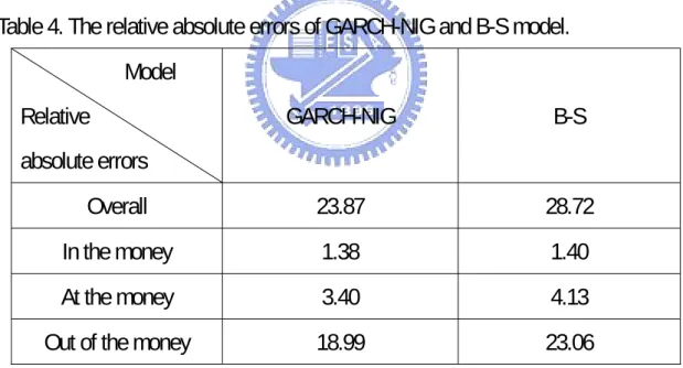
Table 4. The relative absolute errors of GARCH-NIG and B-S model. Model Relative absolute errors GARCH-NIG B-S Overall 23.87 28.72 In the money 1.38 1.40 At the money 3.40 4.13

Out of the money 18.99 23.06

Overall:

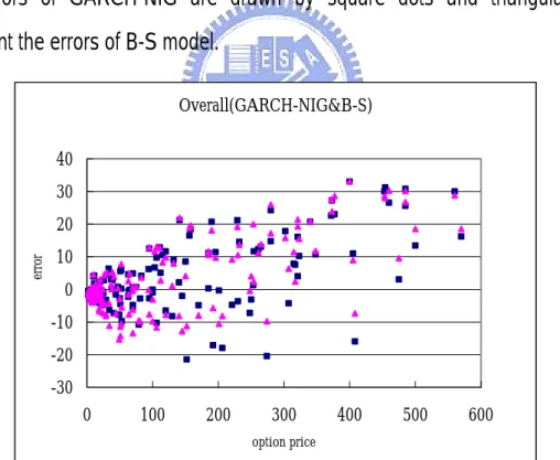
From Table 4 and Figure 4.1, we can see that the relative absolute errors of call option price of GARCH-NIG model is smaller than the B-S model. So the performance of GARCH-NIG model is better than the B-S model. We also see that the higher option price we have, the larger error we get.

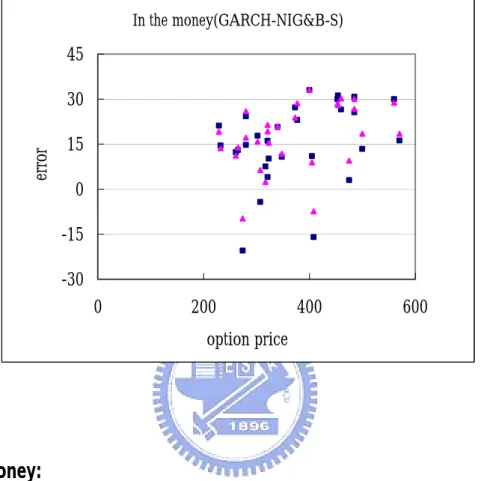
In the money:

We pick up the samples by

s

k <0.95, where is a strike price and is

index. Then we sum all the relative absolute errors of the samples we select and get the following table. From table 4 and figure 4.2, we see that the dispersion of the errors of GARCH-NIG is larger than B-S, but the relative absolute errors of GARCH-NIG is smaller than B-S. So even the “in-the-money” case, the performance of GARCH-NIG is better than B-S, but there are no significant differences.

k s

Figure 4.1. Errors of option price on GARCH-NIG compared with the B-S model. The errors of GARCH-NIG are drawn by square dots and triangular dots represent the errors of B-S model.

Overall(GARCH-NIG&B-S) -30 -20 -10 0 10 20 30 40 0 100 200 300 400 500 600 option price e rror

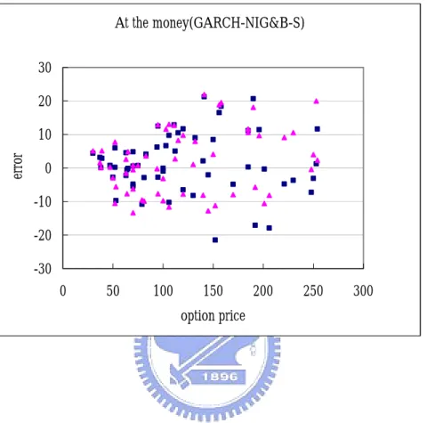
Figure 4.2. Errors of option price on GARCH-NIG compared with B-S model. The errors of GARCH-NIG are drawn by square dots and triangular dots represent the errors of B-S model. In the money(GARCH-NIG&B-S) -30 -15 0 15 30 45 0 200 400 600 option price e rror At the money:

We select the samples by 0.95≤ <

s

k _{1.05, then sum all the relative}

absolute errors. The results are also shown in Table 4 and Figure 4.3.

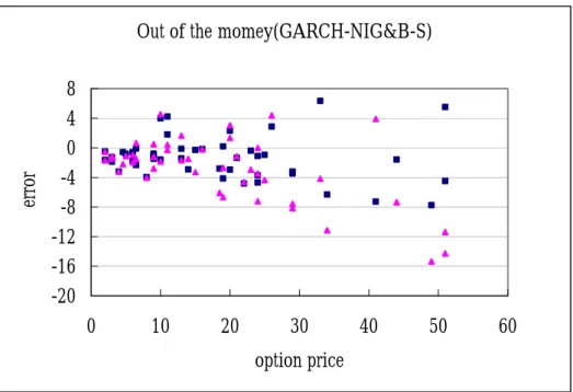
Out of the money:

We select the samples by 1.05

s k

≤ , then sum all the relative absolute

Figure 4.3. Errors of option price on GARCH-NIG compared with B-S model. The errors of GARCH-NIG are drawn by square dots and triangular dots represent the errors of B-S model. At the money(GARCH-NIG&B-S) -30 -20 -10 0 10 20 30 0 50 100 150 200 250 300 option price e rror

Figure 4.4. Errors of option price on GARCH-NIG compared with B-S model. The errors of GARCH-NIG are drawn by square dots and triangular dots represent the errors of B-S model.

Out of the momey(GARCH-NIG&B-S) -20 -16 -12 -8 -4 0 4 8 0 10 20 30 40 50 60 option price error

Figure 4.5. The relative absolute errors in different situations.

0 5 10 15 20 25

In the money At the money Out of the money

Re la tiv e ab so lu te e rr or s GARCH-NIG B-S

From above figures and tables, we can see that there are no significant differences in “in-the-money” situation. But in other situations, like “at-the-money” or “out-of-the-money”, the GARCH-NIG model makes significant improvement in option pricing .Also from Figure 4.5 we can see the relative absolute errors of the BS are higher than GARCH-NIG in different situations. Hence, according to this

research, GARCH-NIG model gets better prediction than B-S model. It means that if we regard the volatility of the return as a constant like B-S model, we may get worse prediction. In other words, if we consider the volatility of the return as a time-variant value, then the error of estimation can be reduced.

5. Conclusions

This paper presents empirical analysis for the price of European call option on the TAIEX using GARCH-NIG model. The GARCH-NIG option pricing model has a number of desirable features and presents a real possibility of correcting the pricing biases associated with the Black-Scholes model.

Appendices:

1. Derive the log likelihood function of GARCH-NIG model.

The probability density function of NIG distribution is given by,

)) ) ( ( ( ) ) ( ( ) exp( ) , ; ( 2 1 1 1 2 1 2 1 2 1

α

α

α

α

π

α

α

h z q K h z q h h z f = − where 2 1 ) (x x

q = + and K1(z) denotes the modified Bessel function of

third order and index one. The log likelihood function is given in the following equation,

∏

= = n i i i t t h z f z L 1 ) ( ) ; , (

α

∑

∑

∑

∑

∑

∑

= = = = = = + + + − − − − = + − + − = = n i t i n i n i t i t n i n i t i t i t n i i t h z K h z h h z q K h z q h z f L 1 2 1 2 1 1 1 2 1 1 2 1 1 2 1 2 1 1 ) ) 1 ( ( ln ) 1 ln( 2 1 ) ln 2 1 ( ) ln ln 2 1 ( )))) ) ( ( ( ln( )) ) ( ( ln( ) ( ln ln 2 1 ( )) ( (ln ln α α α α π α α α α α π α

2. Simulation of normal inverse Gaussian random variables.

We give a way of simulating NIG random variables using the fact that the distribution can be written as a normal variance-mean mixture with mixing function IG. The algorithm looks like this:

(1)Sample RV_t from (

δ

2,

α

2 −

β

2)

IG and let

σ

2 = RV_t,

(2)Sample Y from N(0,1) ,

(3)Return Z = µ + βσ 2 +σY .

The remaining problem is to simulate inverse Gaussian variables. If we write the inverse Gaussian density function as

)) ) ( ( 2 1 exp( 2 ) ( ₂ 2 3 z z z z f_Z

µ

µ

χ

π

χ

− − = where

ψ

χ

µ

= ,then ( ) ~ 2(1) 2 2

χ

µ

µ

χ

Z Z

V = − . Now, let be a realization

of

0

v

V and solve the above quadratic equation for Z. We obtain two solutions

2 0 2 0 0 2 1 4 2 2 v v v z

µχ

µ

χ

µ

χ

µ

µ

+ − + = , and 1 2 2 z z =

µ

, where should be

chosen with probability

1 z 1 z +

µ

µ

and with probability z₂

1 1 z z +

µ

.

References

Andersen TG. 1996. Return volatility and trading volume: an information flow interpretation of stochastic volatility. Journal of Finance 56: 169–204.

Andersen J. 2001. “On the normal inverse Gaussian stochastic volatility model.”

Journal of Business and Economic Statistics 19:44-54.

Andersen TG, Bollerslev T, Diebold FX. 2002. Parametric and nonparametric volatility measurement. In Handbook of Financial Econometrics, Hansen LP, Ait-Sahalia Y (eds). North-Holland: Amsterdam; (forthcoming).

Andersen, T.G. and Sorensen, B.E.(1995),”GMM estimation of a stochastic volatility model : A Monte Carlo study ”, Journal of Business & Economic

Statistics, 14,328-352 (1997),”GMM and QML asymptotic standard deviation in

stochastic volatility models”. Journal of Econometrics, 76,397-403. Barndorff-Nielsen OE. 1978. Hyperbolic distributions and distributions on

hyperbolae. ” Scandinavian Journal of Statistics 5: 151-157.

Barndorff-Nielsen OE, Shephard N. 2002a. “Econometric analysis of realized volatility and its use in estimating stochastic volatility models.” Journal of the

Royal Statistical Society, Series B 64: (forthcoming).

Barndorff-Nielsen OE. 1997. “Normal inverse Gaussian distributions and stochastic volatility modeling.” Scandinavian Journal of Statistics 24:1-13. Barndorff-Nielsen OE, Shephard N. 2001. Non-Gaussian Ornstein – Uhlenbeck -

based models and some of their uses in financial economics, with discussion.

Black, F. & Scholes, M. (1973), ‘The pricing of options and corporate liabilities’,

Journal of Political Economy 81, 637–654.

Bollerslev T, Chou RY, Kroner KF. 1992. ARCH modeling in finance: a review of the theory and empirical evidence. Journal of Econometrics 39: 5–59.

Bollerslev T.(1986): “Generalized Autoregressive Conditional Heteroskedasticity,” J. Economet.,31,307-327.

Bollerslev T. 1987. A conditionally heteroscedastic time series model for

speculative prices and rates of return. Review of Economics and Statistics 69: 542–547.

Boyle, P.(1977): “Options : A Monte Carlo Approach,” J. Financial Econ., 4, 323-338.

Clark PK. 1973. A subordinated stochastic process model with finite variance for speculative prices. Econometrica 41: 135–155.

Engle RF. 1982. Autoregressive conditional heteroscedasticity with estimates of the variance of UK inflation. Econometrica 50: 987–1008.

Jensen MB, Lunde A. 2001. “The NIG-S&ARCH model: a fat-tailed, stochastic, and autoregressive conditional heteroscedastic volatility model.” Econometrics

Journal 4: 319–342.

Jin-Chuan Duan. 1995. ”The GARCH option pricing model.” Mathematical

Finance, Vol. 5, No. 1, 13-32.

Kim S, Shephard N, Chib S. 1998. “Stochastic volatility: likelihood inference and comparison with ARCH models.” Review of Economic Studies 65: 361–393.

L. Forsberg and T. Bollerslev 2002. “Bridging the gap between the distribution of realized(ECU) volatility and ARCH modeling(of the Euro): The GARCH-NIG Model.” Journal of Applied Econometrics 17:535-548

Nelson D. 1991. Conditional heteroscedasticity in asset returns: A new approach.

Econometrica 59: 347–370.

Rubinstein, M. (1985), ‘Nonparametric tests of alternative option pricing models using all reported trades and quotes on the 30 most active CBOE options classes from August 23, 1976 through August 31, 1978’, Journal of Finance 40, 455–480.

Stein, J. (1989), ‘Overreactions in the options market’, Journal of Finance 44, 1011–1023.

Taylor SJ. 1982. Financial returns modeled by the product of two stochastic

processes—a study of the daily sugar prices 1961–75. In Time Series Analysis:

Theory and Practice, Anderson OD (ed.). North-Holland: Amsterdam;

203–226.

Taylor SJ. 1986. Modelling Financial Time Series. John Wiley: Chichester. Tina H. R. 1997. “The Normal Inverse Gaussian Levy Process: Simulation and

Approximation.” COMMUN. STATIST.—STOCHASTIC MODELS, 13(4), 887-910.