國
立
交
通
大
學
電信工程研究所
碩
士
論
文
可抑制旁波瓣與改善增益之半模基板合成波導洩漏
波天線設計
TECHNIQUES FOR SIDE LOBE SUPPRESION AND GAIN
ENHANCEMENT OF A HALF MODE SUBSTRATE INTEGRATE
WAVEGUIDE LEAKY WAVE ANTENNA
研 究 生:呂政皓
指導教授:周復芳 博士
可抑制旁波瓣與改善增益之半模基板合成波導洩漏波天線設計
TECHNIQUES FOR SIDE LOBE SUPPRESION AND GAIN
ENHANCEMENT OF A HALF MODE SUBSTRATE INTEGRATE
WAVEGUIDE LEAKY WAVE ANTENNA
研究生:呂政皓
指導教授:周復芳博士
Student:Jeng-Hau Lu
Advisor:Dr. Christina F. Jou
國 立 交 通 大 學
電信工程研究所
碩 士 論 文
A Thesis
Submitted to Department of Computer and Information Science College of Electrical Engineering and Computer Science
National Chiao Tung University in partial Fulfillment of the Requirements
for the Degree of Master of Science In Communication Engineering
July 2011
Hsinchu, Taiwan, Republic of China
I
可抑制旁波瓣與改善增益之半模基板合成波導洩漏波天線設計
研究生:呂政皓
指導教授:周復芳 博士
國立交通大學電信工程研究所碩士班
中文摘要
使洩漏波天線縮小化並仍能維持應用所需之輻射場型和可以接受增益
是個近年來很具挑戰性的天線設計難題。由於洩漏波天線本身是行波天線,
所以於洩漏波天線上,我們會希望只有正向的行進波於天線結構中存在.
於天線結構任何地方引起的反射波都會對於輻射場型有相當程度的干擾;
但是就算反射波可能可以被完全壓抑,由於洩漏波天線也可被視為是一種
孔徑天線,當一個孔徑天線上近場分布是均勻時,我們仍可以理論上預測
有旁波瓣的存在.這幾點對於洩漏波天線的輻射場型是需要接受改進之處.
基於以上現象,本論文提出一個轉接設計和兩個設計方法以助於改善半模
基板合成波導洩漏波天線的輻射場型和增益.
我們首先提出一個轉接設計以提升饋入洩漏波天線並激發洩漏波模態
的效率.此設計可以較為有效率的激發洩漏波的模態以壓抑於洩漏波天線
端口引起的反射,進而可以避免反射波的激發.此設計對接下來兩個設計
方法具有相當程度的幫助.
II
接下來是提出一個調整半模基板合成波導寬度的方法以達到對旁波瓣
的壓抑.由於這個調整方法能夠改變於洩漏波天線孔徑上的近場分布使其
等效磁流源分佈容易滿足 Taylor's Rules,故旁波瓣可以因而被壓抑.
最後是提出一個回授網路的設計來把洩漏波天線尚未輻射之殘餘能量
導引回洩漏波天線饋入端.如此可以利用其剩餘能量來達到增益的提升.
由於以上設計簡易方便,且容易於所需的頻率點做設計改良,故其在
應用上有很大的潛力.
III
TECHNIQUES FOR SIDE LOBE SUPPRESION AND GAIN
ENHANCEMENT OF A HALF MODE SUBSTRATE INTEGRATE
WAVEGUIDE LEAKY WAVE ANTENNA
Student:Jeng-Hau Lu
Advisor:Dr.Christina F. Jou
Department of Communication Engineering
College of Electrical and Computer Engineering
National Chiao Tung University
ABSTRACT
This thesis gives a study on two techniques to suppress the side lobes and enhance the gain of a half mode substrate integrated waveguide leak wave antenna, respectively.
In this thesis, we are aware of two phenomenon that may spoil the performance of a leaky wave antenna: 1. Due to the traveling wave nature of the leaky wave antennas, the remaining power at the end of the leaky wave antenna should always be carefully guided and terminated or the reflected wave will be excited with the corresponding back lobes that may spoil the radiation pattern. 2. Even if one can guide the wave in the leaky wave antenna to avoid reflections, an ideal leaky wave line source may still introduce side lobes due to the effect of the finite uniform illumination of the aperture antennas. We would here give a study on two methods accompanied with a proposed transition dedicated for a half mode substrate integrate waveguide leaky wave antenna to handle the problems mentioned above.
First, a transition to efficiently convert the input power to construct the leaky mode of the leaky wave antenna is proposed to enhance the efficiency of the leaky wave antenna and avoid possible reflections at the terminal of the leaky wave antenna. This transition can be considered as a stepping stone to facilitate the later analysis and design of the leaky wave antenna.
Secondly, a cosine-shaped tapering profile is proposed to taper the waveguide width of the half mode substrate integrated waveguide. Since one can thus shape the aperture field of the leaky wave antenna to satisfy the Taylor’s rules, the side lobes of the radiation pattern can having a better chance to be suppressed.
IV
Finally, a feed-back network is proposed to guide the non-radiated power back to the feed of the leaky wave antenna. The gain is expected to be enhanced with the aid of the non-radiated power.
These two methods accompanied with the proposed transition can improve the performance of the leaky wave antenna at an arbitrary frequency range easily and thus has great potential in many applications.
V
誌 謝
我之所以能夠於此執筆,首先得感謝我的指導教授周復芳老師,學生在下承蒙老師 不少悉心的照顧,指導和教誨.讓學生在這短暫的碩班期間學到了很多事情,也因此而 有所成長.同時得感謝玠瑝學長這段時間無私的指導提點.讓我對於天線設計這塊領域 有了更深一層的體會和領悟,才進而能讓這篇論文完成. 接著得感謝在919和我一起早上努力奮鬥,晚上打牌打到昏天暗地的學長和同伴 們.感謝超舜學長,智鵬學長,威廉學長和宜星學長這段時間可以不厭其煩地和我討論 並幫助我解決研究上的許多疑惑;感謝曾經和我每天幾乎都忙到看日出的子淵,在關鍵 時刻往往是靠你提醒我容易忽略的盲點,一些危機才能因而變成轉機;感謝小李,阿九, 阿股,以及下一屆的易懋,建榮,小賴和阿牟同我這段研究的苦悶日子一起面對種種的 挑戰.我應該永遠不會忘記和你們晚上一起趕DEAD LINE,一起打桌游,抓著麥克風 高歌的那段時光. 然後需要感謝張嘉展老師、林育德老師、黃瑞彬老師、中正大學無線通訊實驗室的 學長和同學們、交通大學天線遠場量測實驗室的同學們、交通大學電磁晶體研究實驗室 的學長和同學們以及國家晶片中心的學長們對於天線的實作和量測儀器設備上的支持 以及經驗的分享,這篇論文才得以完整;也要感謝王健仁老師和吳俊緯學長在口試階段 給予寶貴的指導和建議,論文才能於此做更進一步的完善. 最後我要感謝我的家人.感謝爸爸,媽媽,外婆以及老姊在這段艱苦的求學歷程中 一直默默給我的愛和支持.我才可以沒有後顧之憂,有動力堅持到劃下這篇論文的句點. 謹於此把我這最後小小的成果獻給你們. 呂政皓 於交通大學 2011.7VI
Tables of Contents
中文摘要 ...I ABSTRACT ... III 誌 謝 ... V Tables of Contents ... VI LIST OF FIGURES ... VIII LIST OF TABLES ... XIIChapter 1 Introduction ... 1
1.1 Motivation ... 1
1.2 Organization ... 2
Chapter 2 Theories of the Half Mode Micro-strip Leaky Wave Antenna ... 3
2.1 Classical Implementations of the Leaky Wave Antennas ... 3
2.2 Characterization of the Leaky Wave Antenna ... 4
2.3 On the Radiation Pattern of the Leaky Wave Antenna ... 5
2.4 The Micro-strip Leaky Wave Antenna ... 6
2.5 Dispersion Characteristics for the Leaky Mode of the Micro-Strip Line ... 6
2.6 Half width MLWA and HMSIW ... 9
Chapter 3 On the Extraction of the Complex Propagation Constant ... 12
3.1 Numerical Through-Line Method ... 12
3.2 Transverse Resonance Method ... 13
3.2.1 Micro-strip Leaky Wave Antenna ... 14
3.2.2 Half mode Substrate Integrated Waveguide ... 15
Chapter 4 A transition design for the HMSIW ... 17
4.1 Introduction ... 17
4.2 On the Analysis of the Structure ... 20
4.3 Simulation Results, Measurements and Discussions ... 24
Chapter 5 Side lobe suppression by tapering the LWA’s waveguide width ... 30
5.1 The effect of length on LWAs ... 30
5.2 The motivation for tapering the LWA ... 33
5.3 The effect on the variation of LWA’s waveguide width ... 36
5.4 The profile of the proposed tapering ... 38
5.5 Analysis and simulation ... 41
5.6 Measurements and some discussions ... 54
Chapter 6 A feed-back network for the LWA ... 59
6.1 Introduction of the feed-back network ... 59
6.2 Analysis and design considerations of the feedback network ... 61
6.2.1 The analysis and design of the adder ... 62
VII
6.3 Measurements and some discussions ... 70
Chapter 7 Conclusions ... 73
Chapter 8 Future Works ... 74
Appendix A The edge admittance of a micro-strip line ... 75
VIII
LIST OF FIGURES
FIG 2.1 A PERTURBED WAVEGUIDE AS A LEAKY WAVE ANTENNA[7] ... 3
FIG 2.2 THE COORDINATE SYSTEM FOR A LEAKY WAVE ANTENNA ... 5
FIG 2.3 THE RADIATION PATTERN OF A LEAKY WAVE ANTENNA ... 5
FIG 2.4 THE MICRO-STRIP LINE 1ST HIGHER ORDER MODE ... 6
FIG 2.5 NORMALIZED COMPLEX PROPAGATION CONSTANT FOR THE 1ST HIGHER ORDER MODE IN THE MICRO-STRIP LINE (W=15MM, H=0.508MM,ΕR=3.55) ... 7
FIG 2.6 THE ELECTRIC FIELD DISTRIBUTION OF THE MICRO-STRIP LINE’S 1ST HIGHER ORDER MODE[6] ... 9
FIG 2.7 THE MICRO-STRIP LEAKY WAVE ANTENNA WITH A PEC WALL[6] ... 10
FIG 2.8 THE HALF WIDTH MICRO-STRIP LEAKY WAVE ANTENNA[6] ... 11
FIG 2.9 HALF MODE SUBSTRATE INTEGRATED WAVEGUIDE[4] ... 11
FIG 3.1 THE EQUIVALENT 2-PORT NETWORK OF THE LEAKY WAVE ANTENNA AND THE ILLUSTRATION OF "THROUGH" AND "LINE" ... 12
FIG 3.2(A) THE CROSS SECTION OF THE MICRO-STRIP LINE[5].(B)THE TRANSVERSE EQUIVALENT CIRCUIT OF ITS LEAKY MODE ... 14
FIG 3.3(A)THE CROSS SECTION OF HMSIW AND ITS EQUIVALENT MODEL[1](B)THE TRANSVERSE EQUIVALENT CIRCUIT OF THE LEAKY MODE ... 15
FIG 3.4 THE COMPARSION OF THE NUMERICAL(HFSS) T-L METHOD AND THE TRANSVERSE RESONANCE METHOD ... 16
FIG 4.1 FRONT VIEW OF A HMSIW LEAKY WAVE ANTENNA ... 17
FIG 4.2 A TRANSITION FOR A SIW (PROPOSED IN [2]) ... 18
FIG 4.3 CONFIGURATION OF THE PROPOSED TRANSITION INTEGRATED WITH THE HMSIW ... 18
FIG 4.4 CONFIGURATION OF THE ENTIRE HMSIW LWA ... 19
FIG 4.5 EFFECT OF THE VARIATION OF W_TRANSTUB ON THE REFLECTION COEFFICIENT ... 21
FIG 4.6 EFFECT OF THE VARIATION OF W_TRANSTUB ON THE FORWARD TRANSMISSION COEFFICIENT ... 21
FIG 4.7 EFFECT OF THE VARIATION OF QL_TRAN ON THE REFLECTION COEFFICIENT ... 22
FIG 4.8 EFFECT OF THE VARIATION OF QL_TRAN ON THE FORWARD TRANSMISSION COEFFICIENT ... 22
FIG 4.9 THE EFFECT OF THE TRANSITION ON THE 2-PORT S-PARAMETERS ... 23
FIG 4.10 MODAL ELECTRIC FIELD(Z) DISTRIBUTION OF THE HMSIW (A) WITHOUT & (B) WITH THE TRANSITION ... 23
FIG 4.11 THE FABRICATED HMSIW LWA PROTOTYPE ... 24
FIG 4.12 COMPARSION BETWEEN THE MEASURED AND SIMULATED 2-PORT S-PARAMETERS ... 24
FIG 4.13 COMPARISON OF THE RADIATION PATTERN IN XZ PLANE AT 5.4GHZ ... 26
FIG 4.14 COMPARISON OF THE RADIATION PATTERN IN XZ PLANE AT 5.6GHZ ... 26
IX
FIG 4.16 COMPARISON OF THE RADIATION PATTERN IN XZ PLANE AT 6.0GHZ ... 27
FIG 4.17 COMPARISON OF THE RADIATION PATTERN IN XZ PLANE AT 6.14GHZ ... 28
FIG 4.18 COMPARISON OF THE RADIATION PATTERN IN XZ PLANE AT 6.2GHZ ... 28
FIG 4.19 ILLUSTRATION OF THE PARAMETER STUDY FOR EXAMINING THE EFFECT OF FINITE GROUND SIZE ... 29
FIG 4.20 THE EFFECT OF TRANSVERSE GROUND SIZE ON THE NORMALIZED RADIATION PATTERN AT 6 GHZ ... 29
FIG 5.1 THE LWA STRUCTURE[4] AND THE EQUIVALENT MAGNETIC LINE SOURCE DISTRIBUTION ... 31
FIG 5.2 COMPARISON OF THE SIMULATED, MEASURED RADIATION PATTERN AND EQ(5.1) ... 32
FIG 5.3 THE DISPERSION RELATIONS AND THE EFFECT OF TAPERING THE WIDTH OF LWA ... 37
FIG 5.4 THE EFFECT OF WIDTH TAPERING ON THE COMPLEX PROPAGATION CONSTANT OF THE LWA ... 37
FIG 5.5 THE PROPOSED TAPERING PROFILE ... 38
FIG 5.6 THE PREDICTED DISTRIBUTION OF ATTENUATION CONSTANT WHEN USING EQ(5.8) AS THE TAPERING PROFILE ... 40
FIG 5.7 THE PREDICTED DISTRIBUTION OF PHASE CONSTANT WHEN USING EQ(5.8) AS THE TAPERING PROFILE ... 40
FIG 5.8 THE CONFIGURATION OF THE TAPERED HMSIW LWA ... 42
FIG 5.9 THE EFFECT OF TAPERING ON THE 2-PORT S-PARAMETERS ... 44
FIG 5.10 THE EFFECT OF TAPERING ON THE RADIATION PATTERN ON XZ PLANE AT 5.40 GHZ ... 45
FIG 5.11 THE EFFECT OF TAPERING ON THE RADIATION PATTERN ON XZ PLANE AT 5.60 GHZ ... 45
FIG 5.12 THE EFFECT OF TAPERING ON THE RADIATION PATTERN ON XZ PLANE AT 5.80 GHZ ... 46
FIG 5.13 THE EFFECT OF TAPERING ON THE RADIATION PATTERN ON XZ PLANE AT 6.00 GHZ ... 46
FIG 5.14 THE EFFECT OF TAPERING ON THE RADIATION PATTERN ON XZ PLANE AT 6.14 GHZ ... 47
FIG 5.15 THE EFFECT OF TAPERING ON THE RADIATION PATTERN ON XZ PLANE AT 6.20 GHZ ... 47
FIG 5.16 EFFECT OF TAPERING ON THE MAGNITUDE OF THE SIDE LOBES ... 48
FIG 5.17 EFFECT OF THE VARIATION OF WD ON THE 2-PORT S-PARAMETERS ... 48
FIG 5.18 EFFECT OF THE VARIATION OF WD ON THE MAGNITUDE OF THE SIDE LOBES ... 49
FIG 5.19 EFFECT OF WD ON THE PEAK OF GAINPHI ON XZ PLANE ... 49
FIG 5.20 EFFECT OF TAPERING ON THE ORIENTATION OF THE MAIN BEAM ... 50
FIG 5.21 ILLUSTRATION OF THE REFERENCE STRUCTURE OF THE TAPERED LWA ... 50
FIG 5.22 COMPARISON OF THE RADIATION PATTERN FOR THE TAPERED LWA AND THE REFERENCE LWA STRUCTURE AT 5.40 GHZ ... 51
FIG 5.23 COMPARISON OF THE RADIATION PATTERN FOR THE TAPERED LWA AND THE REFERENCE LWA STRUCTURE AT 5.60 GHZ ... 51
FIG 5.24 COMPARISON OF THE RADIATION PATTERN FOR THE TAPERED LWA AND THE REFERENCE LWA STRUCTURE AT 5.80 GHZ ... 52
X
FIG 5.25 COMPARISON OF THE RADIATION PATTERN FOR THE TAPERED LWA AND THE
REFERENCE LWA STRUCTURE AT 6.00 GHZ ... 52
FIG 5.26 COMPARISON OF THE RADIATION PATTERN FOR THE TAPERED LWA AND THE REFERENCE LWA STRUCTURE AT 6.14 GHZ ... 53
FIG 5.27 COMPARISON OF THE RADIATION PATTERN FOR THE TAPERED LWA AND THE REFERENCE LWA STRUCTURE AT 6.2 GHZ ... 53
FIG 5.28 THE FABRICATED HMSIW LWA WITH TAPERING ... 54
FIG 5.29 COMPARISON OF THE MEASURED AND THE SIMULATED 2-PORT S-PARAMETERS OF THE TAPERED LWA (WD=0.5MM) ... 55
FIG 5.30 COMPARISON OF THE SIMULATED AND MEASURED PEAKGAIN_PHI FOR THE PROTOTYPE AND THE TAPERD LWA ... 55
FIG 5.31 COMPARISON OF THE MEASURED AND SIMULATED RADIATION PATTERN OF THE TAPERED LWA (5.4GHZ @XZ PLANE) ... 56
FIG 5.32 COMPARISON OF THE MEASURED AND SIMULATED RADIATION PATTERN OF THE TAPERED LWA (5.6GHZ @XZ PLANE) ... 56
FIG 5.33 COMPARISON OF THE MEASURED AND SIMULATED RADIATION PATTERN OF THE TAPERED LWA (5.8GHZ @XZ PLANE) ... 57
FIG 5.34 COMPARISON OF THE MEASURED AND SIMULATED RADIATION PATTERN OF THE TAPERED LWA (6.0GHZ @XZ PLANE) ... 57
FIG 5.35 COMPARISON OF THE MEASURED AND SIMULATED RADIATION PATTERN OF THE TAPERED LWA (6.14GHZ @XZ PLANE) ... 58
FIG 5.36 COMPARISON OF THE MEASURED AND SIMULATED RADIATION PATTERN OF THE TAPERED LWA (6.2GHZ @XZ PLANE) ... 58
FIG 6.1 (A) A EQUIVALENT CIRCUIT FOR A LWA AND (B) THE BLOCK DIAGRAM ILLUSTRATING THE FEED-BACK NETWORK ... 60
FIG 6.2 A RAT-RACE COUPLER DESIGNED FOR A CRLH LEAKY WAVE ANTENNA ... 61
FIG 6.3 ILLUSTRATION OF THE PROPOSED FEED-BACK NETWORK FOR THE LWA ... 61
FIG 6.4 CONFIGURATION OF THE COUPLER IN THE FEED-BACK NETWORK ... 66
FIG 6.5 THE ENTIRE STRUCTURE OF THE LWA INTEGRATED WITH THE FEED-BACK NETWORK . 66 FIG 6.6 THE SIMULATED STRUCTURE TO FIND THE OPEN LOOP EFFICIENCY OF THE LWA ... 66
FIG 6.7 THE S-PARAMETERS(MATCHING AND ISOLATION) OF THE DESIGNED COUPLER. ... 68
FIG 6.8 THE VERIFICATION OF EQ(6.8)&EQ(6.10) ... 69
FIG 6.9 THE SIMULATED 2 PORT S-PARAMETERS OF THE ENTIRE NETWORK INTEGRATED WITH THE LWA ... 69
FIG 6.10 THE FABRICATED LWA INTEGRATED WITH THE FEED-BACK NETWORK ... 70
FIG 6.11 COMPARISON OF THE 2-PORT S-PARAMETERS BETWEEN THE MEASUREMENT AND THE MODIFIED NETWORK ... 71 FIG 6.12 COMPARISON OF THE RADIATION PATTERN OF THE SIMULATED LWA NETWORK, ITS
XI
OPEN LOOP, AND THE MEASUREMENT OF THE FULL NETWORK ... 72 FIG 6.13 COMPARSION OF THE PEAK GAIN OF THE SIMULATED LWA NETWORK, ITS OPEN LOOP,
AND THE MEASUREMENT OF THE FULL NETWORK ... 72 FIG 8.1 CASCADED LWAS WITH FEED-BACK NETWORKS ... 74
XII
LIST OF TABLES
Table 1 Parameters of the LWA prototype………..…19 Tabel 2 The parameters of the tapered LWA and the corresponding reference structure………..………50 Tabel 3 Parameters of the LWA network………58
1
Chapter 1 Introduction
1.1 Motivation
Using a Half-mode substrate integrated waveguide (HMSIW) [1-3] to implement a leaky wave antenna [4-6] can be a convenient choice for antenna designers when a highly directive radiation pattern is required for an antenna on a low-profiled printed circuit board. Since the leaky wave antenna’s (LWA) radiation pattern is simply a narrow beam which we even have means to steer it to a required direction, it can be a good candidate for the radar system and the satellite communication.
However, classical implementations of a LWA requires its longitudinal length to be longer than the order of 5~10λ [7], making the cost too expensive to implement. If we merely fabricate a LWA having a longitudinal length not long enough with an open-end termination, the unwanted reflections at the terminal of the LWA may occur with corresponding “back lobes” to spoil the pattern. On the other hand, a LWA with an aperture length too small will not be practical since the gain and the orientation of the main beam may not easily satisfy the design requirements.
Even if the reflections are properly suppressed, an ideal uniform LWA without reflected waves will still having a side lobe level >-15dB since the LWA’s aperture field distribution is still not well-shaped. The corresponding equivalent line source distributions will theoretically having a radiation pattern with a side lobe level that is not weak.
In this thesis, we try to give a study on realizing a LWA with its length at the order of 1~2λ in order to maintain an acceptable gain. We will here propose a transition for a HMSIW LWA to efficiently convert the power into the antenna and two simple techniques to improve the LWA’s gain and suppress the side-lobes: The first technique is to perform a cosine-shaped
2
tapering of the LWA’s waveguide width to suppress the side lobes. The second technique is to build a feed-back network and guide the non-radiated power back to the LWA instead of making them reflected at the end of LWA.
1.2 Organization
The thesis will begin with the introduction of the leaky wave antenna and some relating theories and techniques in order to facilitate the later analysis. The content of rest of the chapters will be focusing on the proposed LWA design.
Chapter 1 gives an introduction of the paper. Fundamental theories and properties of the micro-strip leaky wave antennas and its half mode implementations will be summarized in chapter 2. In order to understand and control the leakage mechanism of a leaky wave antenna. The method to extract the complex propagation constant of the leaky wave antenna is crucial and will be discussed in chapter 3.
The design of the transition will be proposed in chapter 4. Then in chapter 5, a cosine-shaped tapering profile will be proposed to suppress the side lobes. A feed-back network proposed to enhance the gain of the LWA which has been studied in chapter 5 will then be designed and discussed in chapter6. The conclusion is finally made in chapter 7. Some promising future works will then be recommended in chapter8.
3
Chapter 2 Theories of the Half Mode Micro-strip
Leaky Wave Antenna
In this chapter, we will first give a simple introduction on the characteristic of the leaky wave antenna. Then the radiation characteristics of the micro-strip leaky wave antenna and its half-mode implementation will be discussed. Finally, a simple discussion on the extraction of the complex propagation constant of the micro-strip leaky wave antenna will be given, which may greatly facilitate further analysis and design on the LWA.
2.1 Classical Implementations of the Leaky Wave Antennas
Leaky-wave antennas (LWAs) have been known and used for more than 70 years [7]. As shown in Fig 2.1, almost all the early implementations of LWAs were based on closed metallic waveguides that were made leaky by introducing perturbations along the side of the waveguide to permit the power to leak away along the length of the waveguide. One can refer to [7] for a detailed summary on some previous approaches.
An advantage of LWAs is that they lend themselves easily to shape the radiation pattern whereby sharp directional beams are obtained at a desired angle. Furthermore, this desired angle may easily be tuned by means of frequency scanning.
4
2.2 Characterization of the Leaky Wave Antenna
Leaky-wave antennas form part of the general class of traveling wave antennas characterized by a modal wave propagating along a perturbed guiding structure[8], of which the perturbation is usually a small aperture on a closed waveguide. If the mode in the
waveguide is a fast wave (β<k0), an improper wave called leaky wave can be launched from
the aperture [9]. As the mode propagates along the longitudinal (guiding) direction with the leaky wave, leaking of energy along the aperture surface can be observed[9]. For later convenience, we would simply name any following waveguide modes that can launch the leaky wave a “leaky mode” [10] since it leaks energy while it’s propagating.
For leaky wave antennas, we usually expect only one leaky mode that would exist in the waveguide could contribute the leakage radiation. One can then model this waveguide as a lossy transmission line characterized by a complex propagation constant kx=βx -jαx , where βx
and αx are the phase constant and the attenuation constant, respectively. This "lossy line" can
also be regarded as an antenna that can contribute radiation toward a specific direction, and the direction is dependent of the phase constant of the lossy transmission line.
5
2.3 On the Radiation Pattern of the Leaky Wave Antenna
Considering a LWA located in the coordinated system as depicted in Fig 2.2. The radiation pattern of the corresponding equivalent leaky line source is typically a fan beam (as shown in Fig 2.3) with its peak occurs at q , where M
1 0 sin ( x) M k b q » - (2.1)
Is usually a good approximation [7](k0 is the wave number of the free space). An important
application of the LWA is to adjust the frequency to vary βx/k0 (The normalized phase
constant), and one can steer the beam to M.
Fig 2.2 The coordinate system for a leaky wave antenna
6
2.4 The Micro-strip Leaky Wave Antenna
The first prototype of micro-strip leaky wave antenna is proposed by Menzel[11]. Some further researches on the nature of leakage mechanism from the first higher order mode of micro-strip line is made by Oliner and Lee[5, 8].Comparing to some classical approaches that requires the molding of a metallic waveguide. The implementation using a micro-strip line is considered to be low profile, less weight, and easier to fabricate.
2.5 Dispersion Characteristics for the Leaky Mode of the Micro-Strip Line
For micro-strip leaky wave antennas (MLWA), one would usually want to excite the 1st
higher order mode of the micro-strip line instead of a quasi-TEM mode. The modal electric field distribution is plotted in Fig 2.4 for reference. We would here give a simple description on the properties of the leaky mode.
Fig2.5 shows the normalized propagation constant for the 1st higher order mode of the
micro-strip line. We will follow the classification by Lin in [12, 13] to divide the frequency range into the following four regions:
7
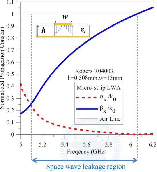
Fig 2.5 Normalized complex propagation constant for the 1st higher order mode in the micro-strip line (W=15mm, h=0.508mm,εr=3.55)
1. ax> ---reactive cutoff region. bx
2. bx>a bx, x< ---surface wave leakage region and space wave leakage region. k0
3. ks>bx> ---surface wave leakage region; k0
4. b > ---bound mode region; x ks
8
When the frequency is low that the mode cannot be constructed, we would say this mode is under reactive cut-off, and a large reflection can be expected if a wave is incident into the “leaky waveguide”. But when the frequency is large enough to build up the mode, since the mode is now a fast wave and the mode permits leakage from the edge of the micro-strip, then leaky space wave can now be launched and starts radiating. When we further increase the frequency, the wave may eventually become a “slow” one and then there is no space wave radiation [12].The usable frequency range for a leaky wave antenna designers often falls in
the space wave leakage region, which we can simply define the lower edge(f )and the upper L
edge( f ) of the usable frequency range: H
( ) ( ) x fL x fL a =b (2.2) 0 ( ) x fH k b = (2.3)
For the case in Fig 2.5, the usable range is approximately 5.1GHz~6.1GHz.
Although the space wave leakage will dominant in the case of the micro-strip leaky mode antenna in this region, the surface wave with zero cutoff frequency is often weakly excited and one should be cautious if this causes the radiation efficiency of the LWA to be lowered.
9
2.6 Half width MLWA and HMSIW
Before discussing the half width MLWA, we would here examine the modal fields of the original higher order mode. Fig 2.6 shows the modal electric fields for the fundamental TEM
and the micro-strip line’s 1st higher order mode. One could here observe the anti-symmetry of
the higher order mode.
A successful design of leaky wave antenna requires an efficient excitation of a single
leaky mode. To be much precise, one should make the best use of incident power to excite a
desired higher order mode of the LWA to make it radiates efficiently.
One of the design difficulties to implement a micro-strip leaky wave antenna should be the presence of the TEM mode, which does not exist in rectangular waveguides. Several
approaches have been used to improve the efficiency to construct the desired micro-strip 1st
higher order mode. These includes periodic transverse slot transitions[11] [14]or via walls[15] inserted in the middle of the micro-strip line to suppress the TEM modes. By observing the asymmetry of the leaky mode’s electric fields, a carefully designed BALUN can be used to feed the micro-strip line at the rightmost and leftmost of the micro-strip’s edge with a nearly 180 phase difference to match the field distribution [16, 17]. Aperture coupling or a CPW-slot-LWA transition [13, 18, 19] have also been studied since the modal fields on the
slot line resembles the micro-strip 1st higher order mode, making the mode can be efficiently
excited.
10
Since the modal field possess anti-symmetry. One may possibly introduce a PEC wall in the middle of the micro-strip line (as shown in Fig 2.7) and remove half of the structure without effecting the original modal field’s distribution(as shown in Fig 2.8). In [6], a half width MLWA is introduced by directly introduce a PEC fence at the middle of the original MLWA and remove half of the micro-strip line. This approach not only effectively suppress the TEM mode due to the PEC walls but also reduce the require width to halves.
The half mode substrate integrated waveguide(HMSIW) which is shown in Fig 2.9 is later being proposed[4] as a novel implementation of a half mode LWA since via walls can also mimic the characteristics of the PEC walls[1-4]. The fabrication of “PEC walls” become easier by simply drill and insert the vias periodically. Equation Section (Next)
11 Fig 2.8 The half width micro-strip leaky wave antenna[6]
12
Chapter 3 On the Extraction of the Complex
Propagation Constant
Since one can predict the radiation pattern with the knowledge of the LWA’s complex propagation constant, it is of most importance to extract them first to facilitate further analysis. In this thesis, two methods will be used to find the complex propagation constant: Numerical T-L method and Transverse Resonance Method.
Fig 3.1 The equivalent 2-port network of the leaky wave antenna and the illustration of "Through" and "Line"
3.1 Numerical Through-Line Method
In this method, we make two “numerical measurements” in a high frequency simulation software (HFSS). To be more specific, we simulate two leaky waveguides with different longitudinal waveguide lengths and “measure” their S-parameters by HFSS. As depicted in Fig 3.1, we assume that the entire LWA structure can be modeled as a lossy transmission line cascaded with error boxes at the beginning and the end. These error boxes can be considered as equivalent circuits that lumps all the discontinuity effects between the terminal port and the
13
structure with length = l1 and l2, respectively, then we can calculate the complex propagation
constant kx= x - jαx with the formula[20]:
2 1 2 2 2 2 2 2 2 2 ( ) 12 12 11 11 12 12 11 11 12 12 12 12 ( ) [ ( ) ] (2 ) 2 x jk l l L T T L L T T L L T e L T - - = + - - + - - -. (3.1)
When we are using this method to find complex propagation constant, there are two things need to be mentioned:
1. We choose l1³0.25landl2£0.5l to prevent some possible numeric errors[21]. 2. The simulated structure must be designed to prevent the excitation of other modes (TEM,
or other higher order ones),or the solution may be corrupted by the modal couplings. In other words, accuracy of the solution can be expected to be increased if we can excite the leaky mode alone much efficiently.
3.2 Transverse Resonance Method
Y
2 2 2 0
x r y
k =ek -k (3.2)
With ky should satisfy the resonance condition[22]:
( ) ( ) 0
Left y Right y
Y k +Y k = (3.3)
YLeft and YRight are the input admittances observed from an arbitrary node of the transverse
equivalent network. We will seek for solutions of ky satisfying eq(3.3) since it would lead to
the answer of kx, which is the complex propagation constant of the mode we are interested in.
The equation is usually nonlinear so one must employ some root searching procedures to find the desired kx.
14
3.2.1 Micro-strip Leaky Wave Antenna
Fig 3.2 shows the transverse equivalent network for a MLWA with full width.One could then enforce the resonance condition to be
cot( ) tan( ) 0 2 2 y t t j w j k Z Z c - +- = (3.4)
The parameter χ in the expression of the input admittance in eq(3.4) is derived from an approximation of a rigorous Wiener-Hopf technique[23, 24]. One can refer to appendix A for a detailed description. The numerical results are shown in Fig2.5.
(a) (b)
15
3.2.2 Half mode Substrate Integrated Waveguide
Since we are using via walls to replace the PEC walls, a modified waveguide model must be used with care to increase the accuracy of the transverse equivalent network model. An empirical model (as shown in Fig 3.3) and formula is available to model the HMSIW as a waveguide with a “perfect short wall” [1, 3]:
2 2 0.54 0.05 2 eff d d w w s w = - + (3.5)
Where w is the physical width, d is the diameter of the via, and s is the spacing between the center of the adjacent vias. The corresponding resonance condition is
cot( ) tan( ) 0 2 y eff t t j j k w Z Z c - +- = (3.6) (a) (b)
Fig 3.3(a)The cross section of HMSIW and its equivalent model[1](b)The transverse equivalent circuit of the leaky mode
16
The numerical results are shown in Fig 3.4. It can be observed that the dispersion relations extracted from these two methods are not quite the same. We think that phenomena are due to some inaccuracies on the modeling of the proposed transverse resonance formulation. The numerical T-L method shall lead to a much reliable result since it is obtained from a rigorous full-wave solver. But the formulation is still considered useful since it would allow for a fast prediction on the range of the space wave leakage region. After these analysis, the space wave leakage region for w=7.5mm can thus be determined on Fig 3.4 accompanied with eq(2.3),eq(2.4) to be approximately 5.3 < f < 6.2GHz.
17
Chapter 4 A transition design for the HMSIW
A transition design for better convert the micro-strip line input power to the desired leaky mode of half mode substrate integrated waveguide (HMSIW) is here being proposed. The purpose of the transition is to construct the leaky mode at the terminal of LWA much efficiently in order to facilitate the further design of the LWA system.
4.1 Introduction
Fig4.1 shows the prototype of a HMSIW as the half width MLWA (HMLWA). We are using Rogers R04003 as the substrate of the circuit board with a substrate thickness = 0.508mm to implement all the HMSIWs throughout the thesis. The aperture length of the LWA is chosen to be 72 mm (~1.4λ). The vias are inserted near the edge of the waveguide periodically to mimic the effect of the PEC wall. After examining the designed rules for a HMSIW[3], the diameter of the via and the distance between adjacent vias are choosen to be 1mm and 2 mm, respectively. The waveguide width of the HMSIW is designed to be 7.5 mm. We assume that port2 can always be terminated with a 50ohm load in order to avoid back lobe problems.
18
Although the classical asymmetric feed (showed in Fig 4.1, with micro-strip attached at the edge of the LWA) can be considered as a simple and direct method to feed the LWA, we would also want to suppress the reflections at the terminal of the LWA due to the discontinuity effects since they may possibly be responsible for some side lobes. A transition which is inspired from a SIW transition [2] (shown in Fig 4.2) is here being proposed to enhance the efficiency to convert the incident power from the micro-strip line to the leaky mode.
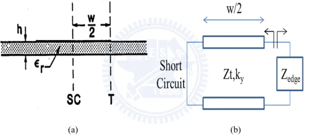
Fig4.3 shows the proposed transition with a stub and a trapezoidal pad connecting the stub and the HMLWA. Fig 4.4 shows the entire leaky wave antenna structure integrated with the transition. The parameters indicated in Fig 4.3~4.4 are tabulated in Table 1.
Fig 4.2 A transition for a SIW (proposed in [2])
19 Fig 4.4 Configuration of the entire HMSIW LWA
Table 1
Parameters of the LWA prototype
w50 1.1mm linelwa1 10mm w50t 1.1mm linelwa2 10mm w_leakline 7.5mm lysubl 30mm w_reserve 1mm lysubr 30mm w_transtub 3.1mm lxsub 107.1mm ql_tran 6mm l_leakline 72mm dvia 1mm svia 2mm
20
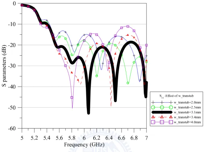
4.2 On the Analysis of the Structure
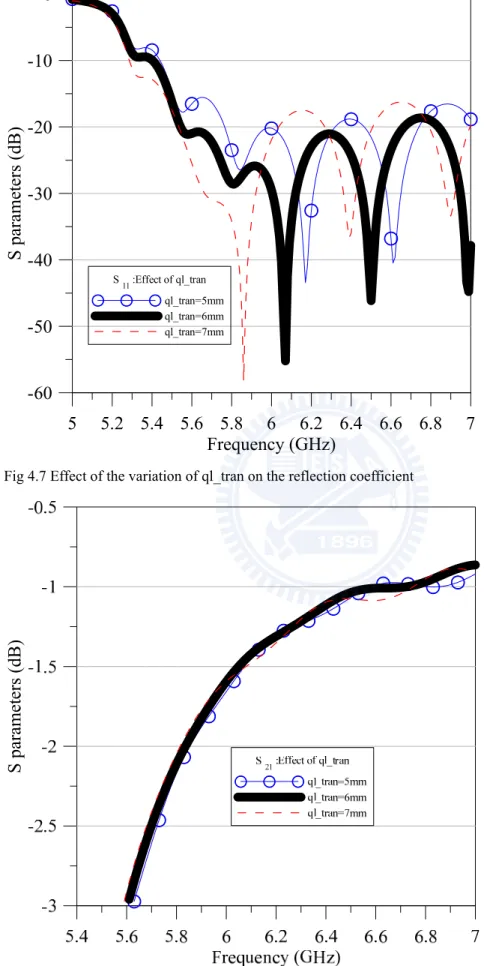
The parameter w_transtub& ql_tran (indicated in Fig 4.3) plays an important role on matching the incident field to the desired leaky modal field. After some studies on the parameters (in Fig 4.5~4.8), w_transtub and ql_tran are choosen to be 3.1mm and 6mm for a better transition design. Fig 4.9 shows the simulated 2-port S-parameters of the HMLWA with & without the transition. A good improvement on the return loss and insertion loss can be observed. One can also be faithful of the transition by observing the modal electric fields (z direction) in the LWA (Fig 4.10 and Fig 4.11). Since some incident power are used to excite the via of the stub scattering cylindrical waves, the scattered wave together with the incident TEM wave can better construct the leaky mode. We are here be convinced that this transition can better convert the micro-strip’s quasi TEM mode to the leaky mode, and this transition would facilitate our further designs of the LWA system.
21
Fig 4.5 Effect of the variation of w_transtub on the reflection coefficient
Fig 4.6 Effect of the variation of w_transtub on the forward transmission coefficient
Sp ar ame te rs( dB) Sp ar ame te rs( dB)
22
Fig 4.7 Effect of the variation of ql_tran on the reflection coefficient
Fig 4.8 Effect of the variation of ql_tran on the forward transmission coefficient -60 -50 -40 -30 -20 -10 0 Sp ar ame te rs( dB) 5 5.2 5.4 5.6 5.8 6 6.2 6.4 6.6 6.8 7 Frequency (GHz) S11:Effect of ql_tran ql_tran=5mm ql_tran=6mm ql_tran=7mm Sp ar ame te rs( dB)
23 Fig 4.9 The effect of the transition on the 2-port S-parameters
Fig 4.10 Modal electric field(z) distribution of the HMSIW (a) without & (b) with the transition
S
parameters
24
4.3 Simulation Results, Measurements and Discussions
The prototype(as shown in Fig 4.11) and the following HMSIWs are fabriacted using a PCB carving machine with the vias drilled and electroplated in advance. The comparison between the measured and the simulated S-parameters of the LWA with transition is shown in Fig 4.13. A fair agreement between simulated and measured results can be observed.
Fig 4.11 The fabricated HMSIW LWA prototype
25
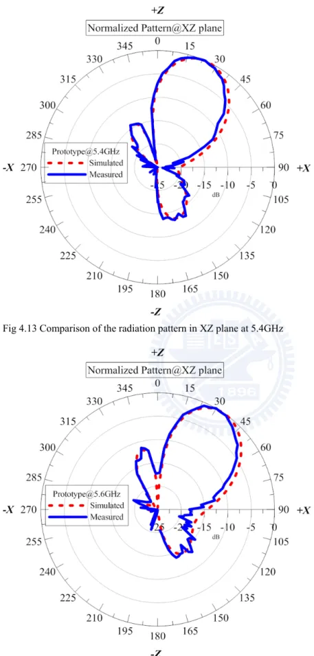
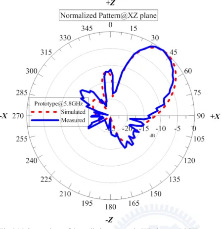
Fig 4.14~19 shows the comparison of the simulated and measured radiation pattern(gainPhi). As can be seen in the results, there is a side lobe above the horizon (+z directions) which steers with the main lobe. It is considered as a defect of a LWA and we will try to solve the problem in chapter 5.
On another hand, a side lobe located below the horizon (-z directions) which steers with the main lobe can be observed. We think that the presence of this lobe is mainly due to the finite transverse ground size (The finiteness of parameter lysubl, lysubr). Theoretically, if the ground is infinite, then direction of power leakage can only allowed to be above the horizon (+z directions).Since for practical application, the ground must have a finite size. Then the energy will be allowed to leak below the horizon. For a finite-length leaky line source placed at the horizon. The leakage toward symmetrical directions with respect to the horizon can thus
be expected. To be more precise, if the main beam is oriented toward M , then this side lobe
is typically oriented toward 180-M from zenith. In [25] , similar phenomenon is being
observed and we are warned to keep the transverse ground width not too small. We try to examine this statement by giving a parameter study on the ground plane size (as shown in Fig 4.19) at 6GHz. The resulting radiation pattern as shown in Fig 4.20 tells us that when we try
to shrink the transverse ground plane width = lysub, a lobe toward 180-M from zenith will
grow and its amplitude may eventually be close with the main lobe. So when we keep the
transverse ground width to be of moderate size, the side lobe toward 180-M can be expected
to be suppressed.
To be short, we are not surprised with this lobe due to the finite ground size and will not put much attention to it. In this thesis, we would mainly deal with possible side lobes that are above the horizon.
26
Fig 4.13 Comparison of the radiation pattern in XZ plane at 5.4GHz
27
Fig 4.15 Comparison of the radiation pattern in XZ plane at 5.8GHz
28
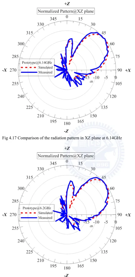
Fig 4.17 Comparison of the radiation pattern in XZ plane at 6.14GHz
29
Fig 4.19 Illustration of the parameter study for examining the effect of finite ground size
Fig 4.20 The effect of transverse ground size on the normalized radiation pattern at 6 GHz
30
Chapter 5 Side lobe suppression by tapering the
LWA’s waveguide width
In this chapter, we attempt to shape the LWA’s radiation pattern by tapering the waveguide width of the LWA. We hope the proposed tapering profile can eventually shape the radiation pattern to achieve a lower side lobe level.
5.1 The effect of length on LWAs
Although the approximation formula eq(2.1) gives a fairly good prediction on the radiation pattern of a LWA, but the effect of the finite aperture length of LWA should also be considered since it would strongly affect the radiation pattern and gain of the LWA. A deeper analysis on the radiation characteristics of a finite length LWA will be necessary.
LWAs are typically traveling wave antennas. Since one can usually treat travelling wave type antennas as aperture type antenna. Some theories and technique to analyze an aperture antenna can be applied on the analysis of LWAs.
By the equivalence theorem[9], one usually can replace the structure of an aperture antenna as an equivalent magnetic current source distribution. Take the HMSIW LWA (shown in Fig 5.1 ) as an example. The entire LWA structure can be replaced by an equivalent
magnetic line current source M(x)=Mx(x) which is continuously distributed along the aperture
of the LWA, and the magnitude of the line source distribution is directly proportional to the aperture near field Ez(x). When the line source distribution is determined, the radiation pattern
R(θ) can then be estimated by evaluating the radiation integral[5]:
0 2 ' 0.5 'sin 2 0 ' 0.5 ( ) x L ( ') jk x ' cos x L R q k = M x e qdx q
=-ò
(5.1)31
Assuming a LWA is being excited that no reflected wave occurs in the LWA structure. Then the aperture field distribution can be approximated to be M x( )e-axxe-j xbx . After substitute M(x) into eq(5.1) , one can find[5]
0 0 0 0 2 ( ) ( ) 0 2 0 2 2 0 0 1 2 cos[( sin ) ] ( ) cos ( ) ( sin ) x x k L k L k k x x x e e k L k R k k a a b q q q a b q - -+ - -+ - (5.2)
We try to plot eq(5.2) in Fig 5.2 as a reference by substituting
0 0
x j x
k k
b a
- ≈0.89-j0.015 @6GHz, which the propagation constant of the HMSIW LWA we just have extracted in chapter 3 with the aid of HFSS. The results are shown accompany with the simulated and measured results in Fig 5.2. It can be seen that the prediction of the radiation pattern by eq(5.1) fairly agrees with the simulation and the measurement. In Fig 5.2, a side lobe which is oriented nearly toward broad side can here be predicted by the simulation and eq(5.1) with a finite magnitude of ~-10dB. Since eq(5.1) is on the ground that the finite reflections in the LWA can be ignored, this phenomenon implies that a LWA can, theoretically, still have side lobe even if the reflected waves are fully suppressed.
32
33
5.2 The motivation for tapering the LWA
The shaping of the aperture field distribution by tapering the parameters of cross section of the perturbed waveguide can be an effective method to reduce the side lobe level. Since again by the equivalence theorem[9], one can replace the leaky aperture as an equivalent line source which is proportion to the field distribution on the aperture. So it would be desirable if one can shape this equivalent current distribution by alter the aperture field distribution in order to modify the radiation pattern.
But then, a question will here arise: which shape of current distribution will help on the side lobe suppression of the radiation pattern? For synthesizing a line source distribution, a theoretical answer has been given by Mr. Tom T. Taylor[26] and his colleagues by listing some important rules to synthesis a line source distribution for a low side lobe radiation pattern, which is called “Taylor’s Rules”. In the “Taylor’s Rules”, a current distribution with 1.A symmetric amplitude distribution and 2.Going linearly to zero at the ends will be recommended since the corresponding radiation pattern produces a lower side lobe envelope. Thus, we should shape the aperture field distribution to satisfy the 2 rules we mentioned above in order to make the equivalent current distribution also satisfy these 2 rules, in order to make the radiation pattern with a lower side lobe level.
Although now we know we would like the aperture field distribution to be a particular shape that we just have mentioned, but how can we do to shape it? Luckily, if the distribution of the attenuation constant along the LWA aperture can be controlled, a synthesis equation for traveling wave antennas can be used[7]:
2 0.5 2 2 1 0.5 0.5 0.5 ( ) ( ) ( ') ' ( ') ' L x Rad L L M x x M x dx M x dx a h -- -=
-ò
ò
(5.3) 2 2 1 (1 / ) 1 LRad t PLoad Pinc e
a
34
The application of this equation is that when the length of the LWA and remaining power (t2) can be estimated, the aperture field distribution can be synthesized to be an arbitrary M(x) by making the distribution of the attenuation constant behaves as this equation.
If we take another glance on eq(5.3), we could find that the factor h , which is Rad
usually defined to be the radiation efficiency of the LWA, plays an important role on the shaping of the attenuation constant. Typically, for a classical LWA design. The aperture length
is designed to be over the order of 5 or more to make the radiation efficiency very close to
unity. But now for our case, we would like to design the LWA with a moderate size so we can only expect the radiation efficiency is poor. This assumption leads to an great simplification of eq(5.3): 2 0.5 2 1 0.5 0.5 ( ) ( ) ( ') ' L Rad L M x x M x dx a h -»
ò
(5.5)Since hRad is here to be very small so the left-side term on the denominator of eq(5.3)
dominates, then if the shaped attenuation constant:
2
( )x M x( )
a µ (5.6)
The shaped equivalent source distribution will be also nearly behaved as M(x). If we here want to shape M(x) to follow the “Taylor’s Rules”, we would also want the distribution of the attenuation constant having a symmetric amplitude and a rapid fall from the center to the edge of the LWA. In other words, we could here expect that if we shape the distribution of the attenuation constant is symmetric from the center of the LWA and having a rapid fall toward the 2 edges of the LWA structure, the side lobe of the LWA’s radiation pattern can be suppressed.
Classical implementation of shaping the attenuation constant is a direct shaping of the LWA’s waveguide cross section parameters. If there exists convenient methods to taper the
35
parameters of the LWA, the synthesizing procedure will be rather straightforward as in[27]. But for micro-strip LWAs, only the width and the height (substrate thickness) of the LWA can possibly be tuned to shape the distribution of the complex propagation constant. Although the possibility to tune the substrate thickness of the LWA has already being studied[28] , it is still considered to be an inconvenient method to realize. Changing the width of the LWA seems to be the only option. Some investigations are here being done to see if we can still suppress the side lobe under this bad situation.
However, we must here be noticed that we should shape the attenuation constant while the phase constant is being fixed. When the distribution of the attenuation constant is changed, the corresponding distribution of the phase constant should be nearly fixed to be a straight line in order to avoid the phase aberration problem[27]. This problem has been studied in [29] by assuming the phase variation along the aperture can be expanded in terms of a polynomial:
2 3
1x 2x 3x ....
f=b +b +b (5.7)
Then for uniform leaky wave antennas, the quadratic (β2) and higher order terms (β3 and the
rest) are zero since the phase constant does not vary with position. The direction of the main
beam will be mainly determined by β1, which can be considered as the average phase constant
along the LWA’s aperture. If we taper the LWA to introduce these higher order terms, β2 is
believed to have minor effects while β3, β4 may contribute to spoil the pattern[29]. In short, the
variation of the phase constant should always be kept to be small, at least not making the effect of β3 and the higher order terms dominate.
36
5.3 The effect on the variation of LWA’s waveguide width
Continued from the analysis in section 5.2, we know that we could try to shape the LWA’s waveguide width to shape the LWA’s attenuation constant in order to suppress the side lobe of the LWA’s radiation pattern. So a preliminary analysis on the effect of changing the LWA’s waveguide width is given as below.
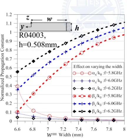
An extensive sequence of numerical T-L method mentioned in Chapter 3 is given to find the complex propagation constant of the LWA with different widths while the substrate is using R04003 with a substrate thickness = 0.508 mm. The numerical results for widths ranging from 6.6mm~8mm are given in Fig 5.3, 5.4. In Fig 5.3, we can see that the usable space wave leakage region of the LWA will suffer a shift to higher frequency band if the width is lowered, and this would also lead to the edge of the reactive cut-off region, which is define as the curve of the phase constant crosses the attenuation constant that we have discussed in Chapter 3, having a shift to higher frequencies. This would imply that some of the frequency range that can be used for frequency scanning applications previously cannot be used now since the shortening of the waveguide width will increase the frequency range of the reactive cut-off region, making the incident wave of the LWA with the same operating frequency will suffer reflections from the LWA since the frequency is now in the reactive cut-off region.
Fig 5.4 gives another representation of the extracted dispersion relations. In Fig 5.4, emphasize is given here on the variance of the complex propagation constant of a single frequency point when we enlarge or shrink the LWA’s waveguide width. When we start to shrink the LWA’ width from w=7.5mm to w=7mm, we can see in Fig 5.4 for the case of f=5.8,6 and 6.2GHz that the attenuation constant will having a linear increase. So we are here confirmed that one can slightly shrink the LWA’s width to increase the distribution of the attenuation constant.
37
Fig 5.3 The dispersion relations and the effect of tapering the width of LWA
38
5.4 The profile of the proposed tapering
Consider the coordinate system as in Fig 5.5, we directly taper the width of the LWA according with the equation (W0, Wd, L are 7.5mm, 0.5mm and 72mm respectively)
0 ( ) dcos( x) W x W W L p = - (5.8)
The profile is depicted in Fig5.2 for reference. Some of the parameters in Fig 5.5 are not drawn in real scale for emphasizing the meanings of the parameters. The reason that we use this equation as the tapering profile can in fact be found in the previous analysis made in section 5.2 and 5.3. Since we should try to change the LWA’s cross section to vary its attenuation constant that its distribution will be even symmetry and having a rapid fall toward the two edges of the LWA This suggest us that we should shape the central distribution of attenuation constant of the LWA to be higher than the 2 edges of the LWA, and we can directly implement this idea by merely shrink the waveguide width in the middle part of the LWA, which this concept is already being verified in section 5.3. So we would use the tapering profile eq(5.8) to taper the LWA’s waveguide width and expect this would lead to the suppression of the LWA’s side lobe level.
39
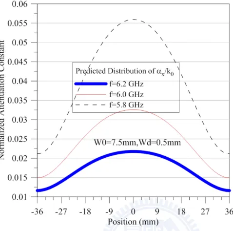
The predicted distribution for the attenuation constant and the phase constant has been plotted in Fig 5.6~5.7 for reference. By using eq(5.8) as the profile, we can see in Fig 5.6 that the predicted distribution of attenuation constant indeed behave as an even function with a sharp roll toward the edge. But we should also here be warned that the tapering profile change the distribution of the phase constant. Since the average phase constant is decreased when the tapering profile is use, we expect this would lead to orientation of the main beam a little bit tilted toward broad side.
To sum these up, we consider the equation eq(5.8) can be a convenient tapering profile to shape the aperture field distribution. Side lobes are here having a better chance to be suppressed.
40
Fig 5.6 The predicted distribution of attenuation constant when using eq(5.8) as the tapering profile
41
5.5 Analysis and simulation
The technique used in the thesis is to sacrifice the scanning range (ranges from 5.3 GHz to 5.6 GHz) from broad side to an angle which is decided by the parameters Wd with the return of a lower side lobe level. Changing the parameter Wd will directly leads to the trade-off between the side lobe level and the usable band width (scanning range) .Since that: 1. When the incident wave enters the tapered LWA, the wave shall deform its field
distribution in order to propagate forward. Leading to the risen of some small reflections along the length of the non-uniform LWA. Moreover, if Wd is chosen to be 0.5 mm, The reflection in the range (5.3 to 5.6 GHz) will be expected to be large since in this range, the waveguide with its width =7.0 mm is under reactive cut-off. A large reflection due to the inability of constructing a leaky mode can then be expected. Although this effect can be suppressed by directly increasing the aperture length in order to make the reflected power (proportion to the remaining power which reaches the smaller waveguide cross section) has smaller amplitude. In the thesis, we will assume that the size restriction is so severe that further increasing the length is impossible to be achieved.
2. On the other hand, if Wd chosen to be big, the distribution of the attenuation constant at the middle will be larger comparing to the distribution at the edge. The side lobe level can be suppressed since the corresponding aperture field distribution is much sharply tapered.
We should here be noted that the traditional tapering profile[16] can better avoids the problems mentioned above since the wave suffers much attenuation by traveling a longer electrical length. The proposed tapering profile will make the wave be reflected mostly at the middle of the LWA while for the case of the traditional tapering profile, the wave will suffer reflections at the end of the LWA.
42
Fig 5.8 shows the tapered LWA structure. Almost all the parameters except the tapered width are kept the same with the prototype mentioned in chapter 4. We use the same parameters for the transition since the transition is originally designed for the same terminal width of the LWA.
Fig 5.8 The configuration of the tapered HMSIW LWA
Fig 5.9 shows the effect of tapering on the 2-port S-parameters. Reflections from 5.3~5.6GHz indeed arise as expected. We are glad to see the reflections at the range at 5.6~6.2GHz is still at an acceptable level, making one can predict that the corresponding (possible) back lobes can be low.
Fig 5.10~5.15 shows the comparison of the radiation pattern between the prototype and the tapered LWA, where the width of the prototype LWA should here again be emphasized to be 7.5mm. Fig 5.16 shows the magnitude of the detected side lobes in the simulated radiation pattern. In this figure, we will only focus on detected side lobes that are above the horizon (|θ|<90deg).Two phenomenon can be observed here:
1. The orientation of the main beam seems slightly tilted toward broad side. We are not surprise with it since the proposed tapering will reduce the waveguide width in an average sense. Making the average of phase constant is reduced in the same frequency point. By eq(2.1), we shall expect this would lead to the beam shifted toward broadside.
43
2. In Fig 5.16, we can see that a side lobe level (considering only the lobes above the horizon) below -18 dB in the entire scanning range is achieved. It can be seen that the side lobes are suppressed due to the tapering in the entire scanning range (5.6 GHz <f<6.2 GHz). Moreover, a nearly 8dB suppression of side lobes in the scanning range 5.8<f<6.2 GHz can be observed, indicating that the proposed tapering profile seems to achieve a surprisingly good result. However, we must here note that the reflections coefficient around the frequency point 5.4 GHz is high; making one should avoid the scanning range at these frequencies. The usable frequency scanning range (5.6~6.2 GHz) is estimated to be 15º<θ<45º from zenith.
A deeper analysis on the effect of changing Wd is given. Fig 5.17 shows the 2-port S-parameters of the tapered LWA with Wd changed to be 0.7mm. It can be seen that a deeper tapering on the LWA’s waveguide results in a smaller scanning range since the reflections at 5.6~5.8 GHz is too large for a practical -10dB requirement. However, the sacrifice of the additional scanning range did get something in return. Fig5.18 shows the magnitude of the side lobe with different “Wd”. It can be seen that a further suppression of the side lobe to the order of -25dB at 6.2 GHz is achieved. The peak gain on XZ plane and the main beam’s angle are also plotted in Fig 5.19~5.20 for reference. It can be seen that the additional tapering results in a gain enhancement of the LWA. Since the tapering can directly increase the attenuation in a brutal way, we can expect this would make more power “lossed” and radiated.
However, the tapering also makes the beam slightly tilted as depicted in Fig 5.20.Or much precisely; the frequency scanning range also suffers a small shift to higher frequencies. This phenomenon cannot be ignored when the LWA is designed for frequency scanning applications. We try to study this phenomenon by finding a reference structure of the tapered HMSIW LWA. We first calculate the average phase constant for the tapered LWA at frequency points 5.4, 5.6, 5.8, 6, 6,14 and 6.2GHz. Then for every frequency point, we find the
44
corresponding LWA’s waveguide width having the same average phase constant and simulate the structure at these frequency points for reference (as depicted in Fig 5.21). Some parameters for the reference waveguide width to compare the tapered LWA are all tabulated in table 2 for reference. The simulated radiation pattern for the tapered LWA and the LWA having the same average phase constant are plotted in Fig 5.22~5.27. Since now the two structures are having the same average phase constant, the orientation of the main beams are almost the same. The advantages of tapering the LWA’s waveguide width will here become apparent that the radiation pattern of the tapered LWA is also having a lower side lobe level comparing to the reference structure. The only defect of tapering that we can see here is a slight enlarge of the lobe width, which is regarded to be a natural consequence when we try to synthesis the aperture field distribution for a radiation pattern having a lower side lobe level[27, 30].
45
Fig 5.10 The effect of tapering on the radiation pattern on XZ plane at 5.40 GHz
46
Fig 5.12 The effect of tapering on the radiation pattern on XZ plane at 5.80 GHz
47
Fig 5.14 The effect of tapering on the radiation pattern on XZ plane at 6.14 GHz
48 Fig 5.16 Effect of tapering on the magnitude of the side lobes
49
Fig 5.18 Effect of the variation of Wd on the magnitude of the side lobes
50 Fig 5.20 Effect of tapering on the orientation of the main beam
Table 2 The parameters of the tapered LWA and the corresponding reference structure Frequency (GHz) 5.40 5.60 5.80 6.00 6.14 6.20 w of the reference structure (mm) 7.118 7.076 7.036 7.034 7.039 7.040
avg(βx/k0)of the tapered LWA 0.1639 0.3087 0.5027 0.6700 0.7640 0.7914
(βx/k0) of the reference structure 0.1637 0.3091 0.5024 0.6699 0.7638 0.7912
avg(αx/k0)of the tapered LWA 0.4003 0.1913 0.0712 0.0341 0.0242 0.0219
(αx/k0) of the reference structure 0.3331 0.1430 0.0495 0.0306 0.0227 0.0208
51
Fig 5.22 Comparison of the radiation pattern for the tapered LWA and the reference LWA structure at 5.40 GHz
52
Fig 5.24 Comparison of the radiation pattern for the tapered LWA and the reference LWA structure at 5.80 GHz
53
Fig 5.26 Comparison of the radiation pattern for the tapered LWA and the reference LWA structure at 6.14 GHz
54
5.6 Measurements and some discussions
The measured and simulated 2-port S-parameters for Wd=0.5mm are plotted in Fig 5.29 for reference. We observed that the measured reflection coefficient seems to be slightly higher than expected. We think this is due to some imperfections on the soldering of the SMA.
Fig 5.30 shows the comparison of the peak gain achieved for the prototype and the tapered LWA. The measured and the simulated results seem to be in a fair agreement. The phenomenon of the gain enhancement due to tapering is also here be verified.
The measured and simulated radiation pattern are plotted in Fig 5.31~5.36 .In the simulation, the pattern in these frequency point achieves a low side lobe level that is <-18dB. However in the measured results, the achieved side lobe level is increased. At the end of the band, the side lobe level for frequency point is only <-15.7dB. We think these lobes may possibly due to the imperfections in the measuring procedure made in the anechoic chamber. In any case, we are here verified the concept of tapering provides a suppressed side lobe level <-15dB.
55
Fig 5.29 Comparison of the measured and the simulated 2-port S-parameters of the tapered LWA (Wd=0.5mm)
56
Fig 5.31 Comparison of the measured and simulated radiation pattern of the tapered LWA (5.4GHz @XZ plane)
57
Fig 5.33 Comparison of the measured and simulated radiation pattern of the tapered LWA (5.8GHz @XZ plane)
58
Fig 5.35 Comparison of the measured and simulated radiation pattern of the tapered LWA (6.14GHz @XZ plane)
Fig 5.36 Comparison of the measured and simulated radiation pattern of the tapered LWA (6.2GHz @XZ plane) Equation Section (Next)
59
Chapter 6 A feed-back network for the LWA
The concept of a feed-back network to recycle the non-radiated power is here being introduced. It contains a branch-line coupler and a 50-ohm micro-strip feed-back delay line loop attached with it. The non-radiated power is designed to be guided back to the feed of the LWA in order to prevent the excitation of back lobe and reuse the power to make it reradiate in the LWA. The gain of LWA is thus expected to be improved.
6.1 Introduction of the feed-back network
Since unwanted back lobes are mainly due to possible reflected waves at the terminal of the LWA, so one will want to suppress the remaining power directly to avoid the back lobe problems. That’s why classical implementations of LWA system require a long longitudinal length over the order of 5λ or even more since the power is here expected to be nearly completely radiated as space waves so little non-radiated power arrives at the end of LWA, making the corresponding back lobes did little pollution to the radiation pattern.
But if we can guide the non-radiated power properly (such as a matched load at the end of the LWA), then the back lobes are likely to be suppressed. This concept leads to the emergence of the feed-back network since it would be intuitive and attractive to guide the non-radiated power and make them radiate. If this concept can be used, one would no longer need to require the longitudinal length of LWA to be very long since one can permit the remaining power to be very large. The required area of LWA can then be reduced. Moreover, we can make use of the remaining power to increase the gain of the LWA.
The concept of feed-back network is in-fact not new. In[31], a feedback network with an amplifier and filter integrated with the feed-back loop is used to make the non-radiated power being amplified and reradiated. In[32], this concept has been extended to shape the radiation pattern by a proper installation of amplifiers along the position of the LWA’s aperture. In [33,
60
34], a novel passive feed-back network consists of a rat-race coupler and a feed-back 50 ohm line loop is been proposed to send back the power to the LWA and make it reradiate. A ~3dB gain improvement over a narrow band is achieved. In this thesis, we extend this concept of feedback network and apply it on a tapered LWA which is designed in chapter 5. We hope the improvement of the gain at the designed frequency can also be observed here.
Fig 6.1 shows the proposed feed-back network diagram in[33]. The network consists of a loop to send the power and an “adder” to gather the original incident power and the non-radiated power. The corresponding output is the sum of these powers and is being guided to the LWA. Since the non-radiated power is here being guided to reradiate. The radiated power and the corresponding gain are expected to be increased. However, as indicated in[33], the adder must accommodate a specific power combining ratio depends on the open-loop LWA efficiency defined in [33]. So the corresponding adder must be properly designed to keep with the open-loop LWA efficiency. The adder proposed in [33, 34] can be a passive directional coupler such as Wilkinson power combiner or rat-race coupler[20, 35]. The center frequency and the power combining ratio of the coupler should be properly designed to meet the requirement of the open-loop efficiency at the frequency of interest.
![Fig 2.7 The micro-strip leaky wave antenna with a PEC wall[6]](https://thumb-ap.123doks.com/thumbv2/9libinfo/8342706.176112/24.892.131.668.528.813/fig-micro-strip-leaky-wave-antenna-pec-wall.webp)