利用子符號內插法實現OFDM通道估計

國 立 交 通 大 學

電信工程學系碩士班

碩士論文

利用子符號多項式內插實現 OFDM 通道估計

OFDM Channel Estimation Based on Sub-symbol

Polynomial Interpolation

研 究 生： 吳柏學

指導教授： 謝世福 博士

利用子符號多項式內插實現 OFDM 通道估計

OFDM Channel Estimation Based on

Sub-symbol Polynomial Interpolation

研 究 生：吳柏學 Student： B. X. Wu

指導教授：謝世福 博士 Advisor： Dr. S. F. Hsieh

國立交通大學

電信工程學系碩士班

碩士論文

A Thesis

Submitted to Department of Communication Engineering

College of Electrical Engineering and Computer Science

National Chiao Tung University

In Partial Fulfillment of the Requirements

For the Degree of

Master of Science

In

Electrical Engineering

July, 2004

Hsinchu, Taiwan, Republic of China

利 用 子 符 號 多 項 式 內 插 實 現 OFDM

通 道 估 計

學生:吳柏學 指導教授:謝世福

國立交通大學電信工程學系碩士班

摘要

在 OFDM 系統的通道估計上，通常藉由訓練訊號 (Training signal)的輔助來找

出通道響應。但考慮到通道的時變性，使用訓練訊號求得的通道響應，並不能代

表資料訊號(Data signal)的通道狀況。在快速衰減的通道下，我們提出子符號多

項式內插方法配合最強路徑選取(most significant taps)演算法來內插出資料訊號

的通道響應。在子符號多項式內插上，將均方誤差分成模型誤差跟雜訊誤差，討

論不同系統參數包括都卜勒頻率，訓練率(Training rate)和多項式階數。我們會

使用一個已知統計特性的通道模型檢查推導出來的誤差與模擬誤差是否配合。最

後拿子符號內插法比較其他現有的多項式內插方法，直接判斷演算法(Decision

OFDM Channel Estimation Based on

Sub-Symbol Polynomial Interpolation

Student: B. X. Wu Advisor: S. F. Hsieh

Department of Communication Engineering

National Chiao Tung University

Abstract

In OFDM channel estimation, we usually utilize training signals. In case of a

time varying channel environment, the channel responses, estimated during

training period, can't represent the channel during data transmission. In such fast

fading channel, we propose the sub-symbol polynomial interpolation algorithm

that retains most significant taps algorithm to interpolate channel responses in data

position. We derives its mean square error (MSE) that includes both model and

noise errors. We verify the MSE performances of the derived results and the

simulation results by using a time varying channel, whose statistics are known.

The proposed sub-symbol polynomial interpolation that is the most effective in the

fast fading channel, compared with the existing polynomial interpolation, the

decision direct algorithm, and the linear interpolation.

Acknowledgements

Firstly, I would like to express my sincere gratitude to my advisor, Dr. S. F. Hsieh,

for his enthusiastic guidance and great patient in my research. Secondly, I also

appreciate all my lab-mates very much for their help. Secondly, I would like to show

my sincere thanks to my family for their encouragement and love. Finally, I want to

Contents

1. Introduction

1

2. Time Domain Approach for OFDM Channel

Estimation

6

2.1 System decription………7

2.2 FPTA channel estimation ………..………...9

2.2.1 FPTA channel estimation algorithm………….……….10

2.2.2 Analysis of channel estimation error of FPTA… ………..………...11

2.3 MST channel estimation ………....12

2.3.1 MST channel estimation algorithm………..13

2.3.2 Analysis of channel estimation error of MST………...………14

2.4 FPTA with LMMSE channel estimation method………....16

3. Time Varying Channel Tracking

19

3.1 Time varying channel model……….………20

3.1.1 DGUS channel model………20

3.1.2 Statistic properties of DGUS channel…...………22

3.2 The FPTA method and The MST method

in time varying channel………...24

3.2.1 FPTA and MST with decision direct algorithm……….25

3.2.1 FPTA and MST with linear interpolation algorithm……….26

3.3 Sub-symbol polynomial interpolation……….……….. 28

3.3.1 Sub-symbol polynomial interpolation algorithm………..29

3.3.2 The MST algorithm for sub-symbol

polynomial interpolation………..………32

3.3.3 Analysis of channel estimation error

of sub-symbol polynomial interpolation………..…….…………33

3.4 Polynomial interpolation of channel

in time-frequency domain………..36

3.4.1 Polynomial interpolation algorithm

in time-frequency domain………..………..37

3.4.2 The comparison between sub-symbol polynomial interpolation and

time-frequency domain interpolation………...………40

4. Computer Simulations

42

4.1 Simulation parameters………42

4.2 Comparison between FPTA, MST and LMMSE

in time invariant channel……..………..43

4.3 Comparison between channel estimation methods

in time varying channel………..46

4.4 Properties of sub-symbol polynomial interpolation………...49

4.4.1 Comparison of different Doppler frequency……….50

4.4.2 Comparison of different training rate………51

4.4.3 Comparison of different polynomial order………52

4.4.4 Comparison of different Channel………..54

List of Figure

2.1

OFDM system block diagram, transmitter and receiver………….…………7

2.2

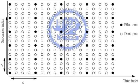
Data grid in time-frequency plane of an OFDM signals………….………….8

3.1

Block of One-tap Recursive Least Square filter……….………….25

3.2

Illustration of linear interpolation………..………..26

3.3

Channel tracking by sub-symbol polynomial interpolation……….…………30

3.4

Data grid in the time-frequency plane of OFDM signals………….…………38

3.5

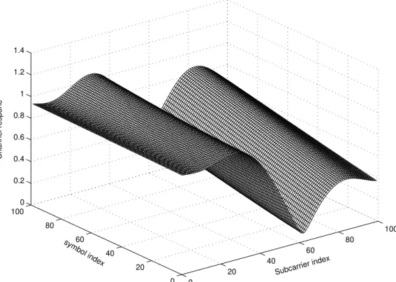
Channel responses distribute in time-frequency plane………….……….41

4.1

Channel estimation mean square error (MSE) in TI Channel-A………...……45

4.2

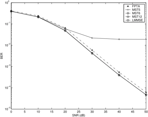
BER performance with different channel

estimation methods in TI Channel-A………...……46

4.3

Channel estimation MSE performance with different threshold

selections in TI Channel-A………..46

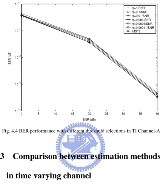
4.4 BER performance with different threshold selections in TI Channel-A…..47

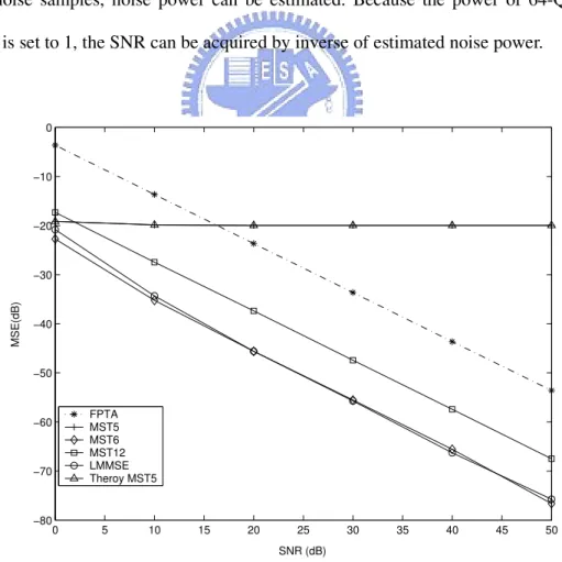
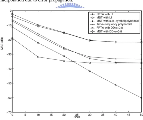
4.5 MSE performance with different channel estimation methods

in Doppler frequency 75Hz environment………48

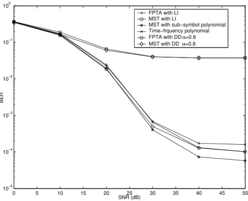
4.6

BER performance with different channel estimation methods in

4.7 BER performance with different taps selection of Combing MST and

sub-symbol polynomial interpolation……….50

4.8 Channel estimation MSE with different Doppler frequencies

in TV Channel-A………51

4.9 Channel estimation MSE with different training rates in TV Channel-A…. 53

4.10 Channel estimation MSE with different polynomial order

in TV Channel-A54………54

4.11 Channel estimation MSE in TV Channel-A and TV Channel-B

Chapter 1

Introduction

Orthogonal frequency division multiplexing (OFDM) has recently become popular due to its desirable properties such as its robustness to intersymbol interference (ISI) and impulse noise, its high data rate transmission capability with high bandwidth efficiency, and its feasibility in application of adaptive modulation and power allocation across the subcarriers according to the channel conditions [1]-[3]. It has been adapted in many applications such as ADSL (Asymmetric Digital Subscriber Line) [4], broadcasting Services such as European DAB (Digital Audio Broadcasting) [5], DVB-T (Terrestrial Integrated Services Digital Broadcasting) [6] and multimedia wireless services such as Japanese MMAC (Multimedia Mobile Access Communication) [7].

The independence among subcarriers simplifies the design of the equalizer and provides an easy method for data recovery. Since the channel information is required in equalization. Channel estimation plays an important role in OFDM system design. Channel estimation is a challenging problem in wireless communications. Because of the mobility of the transmitter, the receiver, or the scattering objects, the channel response can change rapidly with time.

In typical OFDM systems, some part of the transmitted signal is known. In one approach, the transmitter periodically provides known training sequences, which can be used for channel estimation. In a second approach, the pilot channels are provided for channel estimation. This approach is related to the pilot tone approach [8]-[10]. The pilot channels are stronger in power than the information channels.

When there are sufficiently strong pilot channels or sufficient pilot sequence, the channel can be tracked by filtering channel measurements obtained from the pilot information. The filter smoothes the noisy measurements over time and works best when the channel estimate is based on future as well as past channel measurements. Specifically, for a given filter, channel estimation performance depends on the pilot information, fading channel characteristics, and noise level. Pilot information, in term of how much energy and how often it is available, is a tradeoff between minimizing overhead and optimizing channel estimation performance. For example, with pilot symbols, how often symbols must be sent depends on how rapidly the channel is changing.

In channel estimation based on training symbol for time varying channel, some methods need information of statistics of channel [11]-[12]. Channel estimation based on statistics of channel is more complex, but its performance is usually better, depending on the accuracy of the Wiener filter quantities. Channel estimation based on correlation of channel requires knowledge of the statistics of the fading process and the statistics of the measurement noise process. The fading process statistics can be related to parameters of a channel model, such as Doppler spread and average channel coefficient power. Such information is usually unknown. There are many ways to find the statistics of fading process and noise process, but they increase system complexity. The statistics of channel also change with time. The change of

statistics of channel will cause mismatch problem [11]. The performance will be degraded. In order to decrease complexity of channel estimation, we focus on the channel estimation methods without using statistics of channel. One of the simplest forms of channel estimation using pilot symbols is the linear interpolation [13]. With linear interpolation, the channel estimate at a certain time period is a linear combination of the two nearest channel measurements. Linear interpolation can be viewed as applying a filter with symbol-spaced taps to the channel measurements, which contain zeros at the unknown data symbol points. It may get worse channel estimation in cases of high Doppler shift and long distance between training sequence.

We use the polynomial interpolation in this thesis. Compared to the linear interpolation with polynomial interpolation, the polynomial interpolation is more accurate to model a time varying channel. It may have higher complexity than the linear interpolation, but it saves large complexity than the channel estimation based on statistics of channel. The polynomial interpolation can be done in the time domain, in the frequency domain, and in both time and frequency domain [14]-[16]. Some OFDM systems have many subcarriers. There will be a long symbol duration in this system. Channel will is likely to change within one OFDM symbol. We define this rapid change of channel as fast fading channel. The sub-symbol polynomial is proposed for the fast fading channel. The estimation error of sub-symbol is divided into two parts. One is noise error, caused from the noise of the system. The other is model error, which is the difference between real channel impulse and polynomial model. Because the model error is depends on the statistics of channel, we use a time varying channel model in Section 3.1. The statistics of channel will be derived and utilized to check performance of model error. Compared to an existing

time-frequency polynomial interpolation [14] with our proposed sub-symbol method, the latter performs better for two reason. One is the time-frequency polynomial interpolation operated on slow fading channel. It is not suitable to estimate a fast fading channel. The other reason is that the time-frequency polynomial interpolates channel in frequency domain. The channel changes more rapidly in the frequency domain than in the time domain. Interpolation in the frequency domain incurs a larger model error than interpolation in the time domain. In corporating the MST method in [17], the sub-symbol polynomial interpolation only needs to interpolate specific delay taps. It saves more computation than the polynomial interpolation in frequency domain.

Chapter 2 will discuss the channel estimation methods for time invariant channel. The frequency pilot time averaging [17] method will be introduceed first. Then the most significant taps [17] will be introduced to improve channel estimation in time domain. Another improvement of FPTA method, linear minimum mean square [18], is also introduced in Chapter2. The LMMSE method is based on statistics of channel. In simulation results, we can find that the performance of LMMSE is close to the performance of MST. The implementation of MST is easier than LMMSE. MST seems a better channel estimation method than LMMSE. But MST has a problem of selecting proper number of taps. When the numbers of selected taps are less than real numbers of channel taps, Error floor will occur. We also derive the MSE (mean square error) of this error floor in Chapter 2. The channel in Chapter 2 is considered ustationary between two training symbols and equal to the channel of previous training symbol. The channel estimation in one training symbol can be used to recover data.

method for time varying channel based on training symbol will be introduced. The channel estimation in training symbol will be obtained with FPTA or MST. Then we introduce decision directed algorithm [19], linear interpolation, and proposed sub-symbol polynomial interpolation which is used in fast fading channel. We derived the MSE of channel estimation for sub-symbol polynomial interpolaiton method. Its MSE is divided into the noise error and model error. We investigate the sensitivity of the noise error and the model error to different system parameters, including the Doppler frequency, the training rate, the polynomial order and two channel models. We also compare the proposed method with an existing polynomial interpolation in Chapter 3. The simulation results are shown in Chapter 4. In Chapter 5, the conclusion is given.

Chapter2

Channel estimation in time

invariant channel

In this chapter, we will introduce several channel estimation method based on

training symbols. The channel in this chapter is time invariant. The channel can be estimated by using training symbol. The estimated channel can be used to recover data because the channel is time invariant. In Section 2.1, The OFDM configuration is displayed. Because Cyclic Prefix is used in the OFDM system, a simple one-tap equalizer achieves data recovery easily. Then frequency pilot time averaging (FPTA) channel estimation method [17] and its performance are introduced in Section 2.2. The most significant taps (MST) channel estimation method [17] which can improve frequency time domain averaging method [17] is introduced in Section 2.3. The missing tap problem will cause error floor in the performance of MST algorithm. The degredation is also derived in this section. Finally, the linear minimum mean square (LMMSE) channel estimation method [18] is introduced in Section 2.4. The LMMSE channel estimation is also based on the FPTA method. The channel statistics and noise process must be known in the LMMSE method. It is more complex than the MST method.

2.1 System model

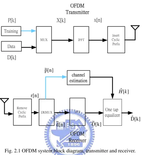
[n] p~ [n] d ~ _D~_[k] Dˆ[k] ] [ ˆ k H r[n]

Fig. 2.1 OFDM system block diagram, transmitter and receiver.

In typical OFDM systems as shown in Fig. 2.1, some part of the transmitted signal is training symbol, the transmitter periodically provides known training symbol,

] [k

X are called frequency domain signals. The frequency domain signals pass the Inverse Fast Fourier Block, then we get the time domain signals x[n]. In order to mitigate ISI effect and keep orthogonal property of sucarriers, The Cyclic Prefix (CP) is added before time domain signal. The time domain signals with CP are transmitted in mobile wireless environment. In the receiver side, we remove CP first. Then the received training signals are picked for channel estimation. Suppose the pilot tonesP[k] are located in a time-frequency plane in Figure 2.1. The training symbols are multiplexed with data symbols in all OFDM symbols at a training rate Pr (ratio

of number of training symbols to number of total symbols). The number of all subcarrier is N and k is subcarrier index. The transmitted training signal in discrete-time domain, excluding CP, can be expressed as

{ [ ]} N

p[n] IFFT P k= (2.1) where IFFTN{} is an N-point inverse Fast Fourier transform of an OFDM symbol and n is the time-domain index, n=0,1,...,N −1. Suppose the wireless channel has a discrete-time impulse response given by

Fig. 2.2 Data grid in time-frequency plane of an OFDM signals

− = − = 1 0 ] [ ] [ L l l l n a n h δ τ (2.2)

where a is called delay coefficient, _l τl is the discrete propagation delay, L is the number of multipaths. In general, the delay coefficient is uncorrelated between different propagation delay paths. This property will be utilized in LMMSE channel estimation method later in this chapter. After passing through a multipath wireless channel, the time domain received samples of an OFDM symbol, if appropriate cyclic

prefix guard samples are used, is given by [ ] [ ] [ ] [ ]

r n = p n ⊗h n +w n (2.3) where ⊗ represents N -point circular convolution, w[n] are independent and identically distributed (iid) AWGN samples with zero mean and variance of 2

w

σ . Assuming perfect synchronization, the FFT output frequency-domain subcarrier symbols can be expressed as

[ ] { [ ]} [ ] [ ] [ ] N R k FFT r n H k P k W k = = + (2.4) where W[k] is Fast Fourier transform of w[n]. Then the channel frequency response at the pilot tones can be estimated by

] [ ] [ ] [ ] [ ] [ ] [ ˆ k P k W k H k P k R k H = = + (2.5)

where k is the subcarrier index of pilot tones. This rough channel estimation is called LS (least square) estimation [17]. If pilot tones don’t occupy all subcarriers, some pilots are zero in the training symbol. The channel responses at those zero tones can be obtained by interpolation.

2.2 FPTA channel estimation

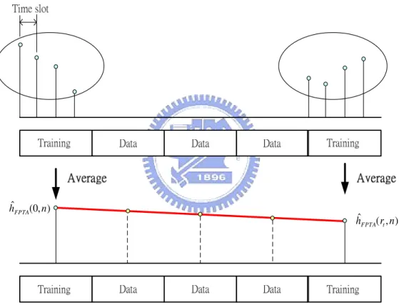
A training symbol can be regarded as several time slots, with each time slot having a pilot. In a slow fading channel or time invariant channel assumption, the impulse response of each time slot is identical. A method can obtain the channel response in the time domain by averaging these time slots. This method is referred to as the Frequency Domain Time Average (FPTA) [17] technique.

2.2.1 FPTA channel estimation algorithm

In FPTA approach, pilot tones are multiplexed with data at a pilot ratio of 1/Kin frequency domain. The frequency domain pilot symbol can be expressed as

− = − = 1 0 ] [ ] [ M m mK k A k P δ (2.6)

where A is the pilot amplitude, k =0,1,...,N −1 and M =N/K is an integer. The corresponding time domain samples contain K identical parts and are given by

− = − = = 1 0 ] [ ]} [ { ] [ K m mM n K A k P IFFT n p δ (2.7)

where n=0,1,...,N −1. The time domain received sample vector of a training symbol can be given by r= ' (2.8) p+w where r=[r₀, r₁,... ,r_K−1 ] , with r_i =[r_i[0],r_i[1],...,r_i[M −1]] , ]] 1 [ ],..., 1 [ ], 0 [ [ − = w w w N

w , p is circular convolution of pilot signal and channel '

impulse response and can be expressed as p'=[ 'p p₀ , '₁ ,...,p_K−1'] with ' [ '[0], '[1],..., '[ 1]]

i = pi pi p Mi −

p . If the maximum channel delay spread is shorter than the length of an time domain identical part, P =i' Pj', for i, j=0,1, ,K−1 and the corresponding parts of received samples are averaged over K parts. This intra symbol time averaging reduce the variance of noise samples by K times. The averaged received samples over K parts is given by

avg K l l avg K r p w r = − = + = ' 1 0 1 0 (2.9)

{w_avg[i]} are iid zero mean complex Gaussian random variables with variance

K

t avg t2, σ2/

σ = . The FPTA [17] time domain channel estimation can be given by

1 ,..., 1 , 0 , ] [ ) / ( ] [ ] [ ) / ( ] [ ˆ − = + = = M n n w A K n h n r A K n h avg avg FPTA _(2.10)

The corresponding frequency response is

Hˆ_FPTA[k]=FFT_N{h_FPTA[n]}, k=0,1,...,N−1 (2.11) Pilot tones lie on several tones of an OFDM system. If we apply channel estimation method in Eq. (2.5), we can only obtain the frequency response of pilot tones. The rest of data tone must be obtained by interpolation. If we use FPTA channel estimation, the channel impulse response can be obtained first and the channel frequency response can be obtained by Fast Fourier transform of the estimated channel impulse response. We don’t need interpolation in frequency domain.

2.2.2 Analysis of FPTA channel estimation error

We define channel estimation error in time domain as ˆ

[ ] _FPTA[ ] [ ] ( / ) _avg[ ]

e n =h n h n− = K A w n . (2.12) The variance of [ ]e n or Mean Square Error (MSE) of channel impulse response can be given as follows 2 2 2 , 2 2 * ]} [ ] [ { ]} [ { ]} [ var{ w avg w A K A K n e n e E n e mse n e σ σ = = = = (2.13)

The corresponding channel estimation error in frequency domain can be obtained by Fast Fourier transform of [ ]e n and can be represented as follows

₋ = − − = − = = = 1 0 / 2 1 0 / 2 ] [ ] [ ]] [ [ ] [ M n N kn j N n N kn j N e n e e n e n e FFT k e π π (2.14)

The variance (MSE) of channel estimation in frequency domain can be written as

2 2 * ]} [ ] [ { ]} [ { ]} [ var{ w A N k E k E E k E mse k E σ = = = (2.15)

In the next paragraph, the MST will be derived. The MSE of FPTA will compare with MSE of MST in next paragraph, and it will be shown that MST performs better than FPTA.

2.3 MST channel estimation

There may not be so many channel paths with significant strength in N samples interval of an OFDM symbol. Hence, among N samples (taps) of channel impulse response estimate, many samples (taps) will have little or no energy at all except noise perturbation. Neglecting those nonsignificant channel taps in channel estimation may introduce some performance degradation if some of the channel energy is missed, but at the same time it will eliminate the noise perturbation from those taps. Total noise perturbation from those neglected channel estimate taps are usually much higher than the mulitpath energy contained in them, especially for low SNR values. Hence, neglecting those nonsignificant channel estimate taps can improve the channel estimation performance significantly. There are two ways to select taps [17]. One is to select several significant taps, and the other is to select the taps which is above a threshold. If we select the channel taps, which are less than the real numbers of the

channel taps, we define this situation as missing tap or under-determined condition. In opposition to the missing taps, the selected channel taps, whose numbers are more than the real ones, are defined as over-determined condition. The error floor will occur in the under determined-condition. It is a serious problem in the performance of channel estimation. In this section, we want to derive the MSE performance of channel estimation under the condition of missing taps.

2.3.1 MST channel estimation algorithm

Training symbol of the MST approach is the same as the FPTA in Eq. (2.6) and Eq. (2.7). It contains K impulses and distributes uniformly in N samples of time domain. If the channel path gains remain essentially the same over an OFDM symbol interval, which is usually the case since OFDM symbol is often designed to satisfy this in order to maintain orthogonality among subcarriers, then the received samples corresponding to time-domain pilot samples contain K repeated version of scaled channel impulse response which are independently corrupted by AWGN. In order to choose most significant channel taps (MST), those K parts can be averaged so that the noise variance is reduced by K times and more reliable most significant channel taps can be obtained. In mathematical expression, the time-domain received samples corresponding to time-domain pilot samples can be given by

− = − = + − = + ⊗ = 1 0 1 ,..., 1 , 0 ], [ ] [ ] [ ] [ ] [ ] [ K m N n n w mM n h K A n w n p n h n r (2.18)

Then averaging the received samples over K parts, we have the noise-corrupted scaled channel impulse response

[ ]= h[n]+w [n], n=0,1,...,M −1

K A n

ravg avg

The FPTA channel impulse response estimation is given by

ˆ [ ]= [ ]= [ ]+ w [n], n=0,1,...,M −1 A K n h n r A K n

hFPTA avg avg (2.19)

After channel impulse response is estimated by the FPTA algorithm, the most significant J channel delay taps are chosen for the MST channel estimation. Suppose the time indices of the most significant J taps are n₀,n₁,...,n_J−1. The MST method is obtained by setting the other channel taps gains to zero as shown below

ˆ [ ] 1ˆ [ ] [ ], 0,1,..., 1 0 − = − = − = N n n n n h n h i J i FPTA i MST δ (2.20) The corresponding frequency response estimation is directly obtained by Fast Fourier transform of hˆ_MST[n]. How to select the number of taps J is an important problem in MST algorithm. In next paragraph, we discuss the selection of J by analysis of MSE for channel estimation.

2.3.2 Analysis of MST channel estimation error

In the mean square error analysis, we consider the over determined condition in which J is larger than total number of delay taps L . Recall Eq. (2.20), the estimated channel impulse response by the MST can be written as

] [ ] [ ] [ ] [ ] [ ˆ ] [ ˆ 1 0 1 0 i J i avg i i J i FPTA i MST n n n w A K n h n n n h n h − + = − = − = − = δ δ (2.21)

j kn N i J i avg i N n MST _A w n n n e K k H k H 1 2 / 0 1 0 ] [ ] [ ] [ ] [ ˆ − _δ − π = − = − + = (2.22)

The MSE in frequency response is

} { } ] [ ˆ ] [ { ]} [ { 2 , 2 2 2 FPTA avg t MST H mse N KJ J A K k H k H E k H mse = = − = σ (2.23)

The MSE performance gain of the MST method over FPTA method is ideally KJ /N. The smaller J gets the better performance of MSE, but J musts larger or equal to

L . The best choice of J is set to L .

Now, we extend the analysis of MSE to under determined condition (J < ). The L

estimated channel impulse response by the MST can be written as

] [ ] [ ] [ ] [ ] [ ] [ ] [ ˆ ] [ ˆ 1 0 1 1 0 i J i avg i m L J m i J i i LS MST n n n w A K n n n h n h n n n h n h − + − − = − = − = − = − = δ δ δ (2.24)

The estimated frequency response can be obtained as follow

N kn j i J i avg i N n N kn j m L J m m N n MST e n n n w A K e n n n h k H k H / 2 1 0 1 0 / 2 1 1 0 ] [ ] [ ] [ ] [ ] [ ] [ ˆ π π δ δ − − = − = − − = − = − + − − = (2.25)

The MSE in frequency response is

} { } ] [ ˆ ] [ { ]} [ ˆ { 1 2 ] [ 2 FPTA L J m hn MST MST H mse N KJ k H k H E k H mse m + = − = − = σ (2.26) where 2 ] [nm h

σ is the power delay profile for the n th propagation delay path. The _m

error floor occurs in this case because of missing tap. The channel estimation error caused by the noise from an additional tap in channel estimation is much less than that caused by missing one tap of the multipaths. The choice of the number of most

significant taps J must be larger than the number of multipaths to prevent channel estimation error caused by missing taps. A suitable choice [17] for J may be two times or more of the number of multipaths. Another MST tap selection can be implemented by selecting the channel taps whose energy is above a threshold [17]. The threshold may be set as η times the maximum channel tap’s energy. In the simulation results, we can find the suitable choice of η depend on the operating SNR. A suitable choice of η is 20dB below 1/SNR. MST improves performance of FPTA by noise suppression. If the channel taps is small. MST algorithm gains more noise suppression by selecting fewer taps. Comparing the outdoor mobile channel with the indoor wireless channel, there are fewer channel taps in the outdoor mobile channel than in the indoor mobile channel. Therefore, the MST algorithm is suitable for the outdoor mobile channel beter than the indoor wireless channel.

2.4 FPTA with LMMSE channel estimation

In Section 2.3, we use MST algorithm to improve FPTA channel estimation. In this section we will introduce another channel estimation method, based on correlation of channel, to improve FPTA channel estimation. This channel estimation method is called LMMSE [18]. The performance of MST with matched selection of taps, selected numbers of taps is equal to the real number of taps, is the same as the performance of LMMSE.

FPTA channel estimation method can also be improved by using linear minimum mean square error (LMMSE) [18]. In LMMSE channel estimation, we need to know the autocorrelation matrix of hˆ_FPTA and the cross correlation matrix between hˆ_FPTA

and h . T FPTA FPTA FPTA FPTA [hˆ [0],hˆ [1], ,hˆ [M 1]] ˆ _{= −}

h is the estimated impulse response

with FPTA. _{h=[h[0],h[1], h[M −1]]}T _{is the true channel impulse response. If we} define the autocorrelation matrix R and cross correlation _{h ˆ}ˆ_h R as hh

} ˆ ˆ { ˆ ˆh FPTA FPTAH h E h h R = (2.28) } { H hh E hh R = (2.29) We can write LMMSE channel estimation [18] as

hˆ_mmse R_hhR_hh1hˆ_FPTA ˆ ˆ −

= (2.30) Lets us consider a wide-sense stationary uncorrelated scattering (WSSUS) multipath channel with power delay profile given by 2

i h

σ at delays of i OFDM sample intervals. Due to the uncorrelated multipaths, the correlation matrix of channel impulse responseR becomes a diagonal matrix with the diagonal elements given by _hh

the power delay profile. The Eq. (2.28) can be rewritten as

FPTA h h h h h h mmse SNR SNR SNR diag N N h h ˆ } / , , / , / { ˆ 2 2 2 2 2 2 1 1 1 1 0 0 β σ σ β σ σ β σ σ + + + = − − (2.31)

where SNR/β in Eq. (2.31) is replaced by 2_(AK)−2

w

σ , 2

w

σ denotes the noise variance in time domain and K is the number of impulses in a training symbol. Compared to MST with LMMSE, LMMSE needs more computation on estimation of

channel correlation and noise power. We can find the performance of MST with matched selection of taps in simulation results is similar to the performance of LMMSE in simulation results. MST has lower complexity than LMMSE, MST seems to be a better choice than LMMSE. But in general, we don’t know how many taps in the channel. In next Chapter, we consider the time varying channel. The decision directed algorithm [19], linear interpolation [13], and polynomial interpolation [14] will be implemented by FPTA and MST. Furthermore, in fast fading assumption, sub-symbol polynomial interpolation is proposed. The sub-symbol polynomial interpolation apply MST algorithm to reduce complexity and do noise suppression.

Chapter 3

Time Varying Channel Tracking

In Chapter 2, we introduced the FPTA method and MST method for channel estimation. They work fine in time invariant channel. In this Chapter, The serious problem, mobile fading channel, in channel estimation will be discussed. The channel impulse responses change in different time slot (One OFDM symbol is divided into several time slots) of one OFDM symbol. The estimated channel impulse response of the training symbol is an improper channel estimation for data symbols in time varying channel assumption. In order to solve this problem, the sub-symbol polynomial interpolation algorithm will be proposed. We suppose every delay tap of impulse response change in every time slot and is close to a polynomial function. The polynomial interpolation utilizes LS channel estimation in training symbol to get the coefficients of polynomial function. Then it interpolates the channel impulse response in data symbol. The estimation error is divided into two parts. One is noise error, caused from the noise of the system. The other is model error, which is generated by the difference between real channel impulse and polynomial model. Because the model error is relative to the statistics of channel, we use a time varying channel model in Section 3.1. The statistics of channel will be derived and utilized to check performance of model error. Furthermore, we can mitigate noise effect of the LS

channel estimation in training symbol by Wiener filter. It makes some improvements for higher-order polynomials. We also compare other existing time varying channel estimation methods in this Chapter including decision directed algorithm, linear interpolation, and time-frequency domain polynomial interpolation. The performance of these channel estimation method will be shown in Chapter 4.

3.1 Time varying channel model

The concept of deterministic channel modeling [20] has recently been extended [21]

to frequency-selective mobile radio channels, resulting in a new class of model processes, called deterministic Gaussian uncorrelated scattering (DGUS) model. The DGUS model can be interpreted as the deterministic counterpart of Bello’s [22] stochastic WSSUS model. We describe DGUS model in equivalent complex baseband. The function of the system and statistics of the model will be introduced latter.

3.1.1 DGUS channel model

The time variant impulse response of the DGUS model is given by a sum of L discrete delay paths, according to

− = − = 1 0 ) ( ) ( ) , ( L l l l l t a t hτ µ δ τ τ (3.1)

where the real-valued a are called delay coefficients, _l µ_l(t) are complex deterministic Gaussian process, and τ_l are discrete propagation delays. Both the delay coefficients a and the discrete propagation delays _l µ_l(t) determine the delay

power spectral density of frequency–selective deterministic channel models. Strictly

speaking, the delay coefficient is a measure of the square root of the average delay

power, which is assigned to the

l

th path discrete propagation path. The channel

disturbance of the Doppler effect, caused by the relative motion between the receiver

and the transmitter, are modeled in Eq. (3.2) by complex deterministic Gaussian

processes.

∑

= +

=

l nl nl N n t f j l n l

t

c

e

1 ) 2 ( . , ,

)

(

π θ

µ

_(3.2)

where 1

l

=

0

,

1

,...,

L

−

.

N denotes the number of harmonic functions, assigned to

l

the

l

th path,

c

_n,l

is the Doppler coefficient of the

n

th component of the

l

th

propagation path, and

f

_n,l

and

θ

_n,l

are the corresponding discrete Doppler

frequency and Phase. The time-varying channel impulse response

h

(

t

,

τ

)

is

completely deterministic. Therefore, the correlation properties of

h

(

t

,

τ

)

are derived

from time average, instead of statistical averages. Figure 3.1 shows the structure of

the complex Gaussian random process

µ

_l

(t

)

in the continuous-time representation.

To ensure that the simulation model which is derived below has the same striking

properties as a uncorrelated scattering (US) model, the complex deterministic

Gaussian processes must be uncorrelated for different propagation delays, i.e., the

deterministic process

µ

_l

(t

)

and

µ

_λ

(t

)

have to be designed in such a way that they

are uncorrelated for

l ≠

λ

, where

l

,

λ

=

0

,

1

,...,

L

−

1

. This demand can be fulfilled

easily if the discrete Doppler frequencies

f

_n,l

are chosen in such a way that the sets

{

±

f

_n,l

} and {

±

f

_m,λ

} are mutually disjoint for different propagation delays. Thus, the

US condition can be expressed by

λ

λ

≠

±

≠

⇔

f

nl

f

m

for

l

, ,

US

(3.3)

where

n

=

1

,

2

,...,

N

l

,

m

=

1

,

2

,...,

N

λ

, and

l

,

λ

=

0

,

1

,...,

L

−

1

.

3.1.1 Statistic properties of DGUS channel

In the following paragraph, we derive the correlation properties of the deterministic

Gaussian process Eq. (3.2)

dt

t

t

T

r

T T l T l

₂

(

)

(

'

)

1

lim

:

)

'

(

τ

µ

*

µ

_λ

τ

µ µ λ

=

_→∞

∫

₋

+

(3.4)

can be expressed in closed form by

_µµ

τ

=

∑

π τ =

λ

= l e c r l l n l l N n f j l n , if ) ' ( 1 ' 2 2 , ,

(3.5a)

r

_µµλ

τ

=

l

≠

λ

l

(

'

)

0

,

if

(3.5b)

where 1

l

,

λ

=

0

,

1

,...,

L

−

. )

_µµλ

(

τ

'

l

r

is the autocorrelation function of the

deterministic Gaussian process

µ

_l

(t

)

defined by Eq.(3.2). Next, we define the Fourier

transform of autocorrelation function of deterministic Gaussian process

_µµ

(

τ

'

)

l l

r

∑

∫

= ∞ ∞ − − = = l l l l l N n l n l n f j f f c d e r f S 1 , 2 , ' 2 ) ( ' ) ' ( ) (

δ

τ

τ

πτ µ µ µ µ

(3.6)

The )

S

( f

lµλ

µ

is called the Doppler power spectral density of the

l

th propagation

path. Without the loss of generality, the area of

S

( f

)

lµλ

µ

over all frequency is equal

to one. The Doppler coefficients

c

n,l

must satisfy the following condition

1 1 2 , =

∑

= l N n l n c

(3.7)

for 1

l

=

0

,

1

,...,

L

−

. In a typical mobile system, the Doppler power spectral density

can be expressed as

⎪ ⎩ ⎪ ⎨ ⎧ ≤ ≤ − = l D l D l D f f f f f f k f S l l , , 2 2 , 0 ) ( µ µ

(3.8)

where

k

is a constant which depends on the average power of the deterministic

Gaussian process

µ

l

(t

)

, and

f

D,l

is the maximum Doppler frequency. Then

combining Eq. (3.6) and Eq. (3.8), we can get the following equation

2 , 2 , 2 , ~ l n l D l n f f k c − =

(3.9)

We also have to satisfy the Eq. (3.7) condition. Finally, the Doppler coefficients

c

_n,l

can be obtained from the discrete Doppler frequencies

f

_n,l

.

∑

=

−

−

=

l N n _{Dl nl} l n l D l n

f

f

f

f

c

1 2_, 2_, 2 , 2 , 2 ,

1

1

~

_(3.10)

where

n

=

1

,

2

,...,

N

l

, 1

l

=

0

,

1

,...,

L

−

.The Doppler power spectral density

S

µµ

( f

)

of DGUS channel can be determined from the Doppler power spectral density for

l

th

propagation path.

∑

− =

=

1 0 2

)

(

)

(

L l l

S

f

a

f

S

l lµ µ µµ

(3.11)

The average Doppler shift of the DGUS model

(1)

µµ

D

is defined by the first moment

of )

S

_µµ

( f

, i.e,

∑ ∑

∑ ∑

∫

∫

− = = − = = ∞ ∞ − ∞ ∞ −

=

=

1 0 1 2 , 2 1 0 1 2 , , 2 ) 1 (

]

[

]

[

)

(

)

(

:

L l N n l n l L l N n l n l n l l l

c

a

c

f

a

df

f

S

df

f

S

f

D

µµ µµ µµ

(3.12)

The Doppler spread

D_µµ(2)

of DGUS model is defined by the square root of the second

central moment of

S

_µµ

( f

)

, i.e.,

2 ) 1 ( 1 0 1 2 , 2 1 0 1 2 , , 2 2 ) 1 ( ) 2 (

)

(

]

[

]

)

(

[

)

(

)

(

)

-(

:

µµ µµ µµ µµ µµ

D

c

a

c

f

a

df

f

S

df

f

S

D

f

D

L l N n l n l L l N n l n l n l l l

−

=

=

∑ ∑

∑ ∑

∫

∫

− = = − = = ∞ ∞ − ∞ ∞ −

(3.13)

3.2 The FPTA and the MST method in time

varying channel

In this section, we introduce two channel estimation methods whose don’t need

statistic of channel in the time varying channel. One is decision direct algorithm, the

other is linear interpolation. In the decision direct algorithm, the initial channel

estimation in training symbol is obtained by FPTA or MST. Then decision direct

algorithm [19] is used to track the channel in the data position. In the linear

interpolation, channel in training symbol is also estimated by FPTA or MST. Then we

do linear interpolation by two neighbor training channel which is estimated with

FPTA or MST.

3.2.1 FPTA and MST with decision direct algorithm

The corresponding channel frequency response estimation of the FPTA method or the MST method is N-points Fast Fourier transform of hˆ_FPTA or hˆ_MST. A simple decision directed method will be introduced. It is called one-tap Recursive Least Squares filter [19]. The algorithm is

) , 1 ( ˆ ) , ( ) , ( ) , 1 ( ˆ ) 1 ( ) , ( ˆ( , ) ) , ( ˆ k m H k m R k m Z k m H k m X k m R k m H − = − − + =α α (3.14)

where R( km, ) is the received symbol at k th subcarrier and mth data symbol; )

, ( ˆ _{m k}

X is the estimation of the constellation at k th subcarrier and m th data symbol; Hˆ(m,k) is the estimation of the demodulated channel; Z( km, ) is the decision variable (a noisy estimate of the constellation value X( km, )) and

α

is the update factor in the estimation of the channel. The algorithm is also shown in Figure 3.1.

α

α

− 1 ) , ( ˆ _mk Z Xˆ(m,k) ) , ( ˆ ) , ( k m X k m R ) , ( km R ( , ) ˆ _mk H ) , 1 ( ˆ _{m k} H −

Fig. 3.1 Block of One-tap Recursive Least Square filter

The initial channel estimation can be completed by training symbol (FPTA or MST), then update the channel by the one-tap Recursive Least Squares filter. Periodic resending of the training symbol will reorient the estimation of the channel to the correct position. The errors will typically occur when the signal is in a deep fade.

3.2.2 FPTA and MST with linear interpolation algorithm

) , ( ˆ _{r n} h_{FPTA t} ) , 0 ( ˆ _n hFPTA

Fig. 3.2 Illustration of linear interpolation

In FPTA or MST methods, we use the channel that is estimated by training symbol

to recover data. The mobile fading channel changes with time. The channel of training symbol is different from the channel of data symbol. Even the channel of training symbol can be estimated very accurately, it still can’t be used to recover data. Fortunately, because the channel doesn’t change rapidly in short-time intervals or in low Doppler frequency mobile environment, then we can suppose that the channel

presents the linear change between two training signals both in the time domain and in

the frequency domain. Figure 3.2 shows the illustration of linear interpolation. First,

we estimate channel of training symbol by FPTA or MST. The estimated channels of

two adjacent training symbols can be used to make a straight line, then we can

interpolate channel of data symbols by this straight line. The linear interpolation [13]

can be carried out in two domains. One is the interpolation in the time domain, which

is achieved by the linear interpolation in delay propagation path. The other is

interpolation in the frequency domain, which is achieved by linear interpolation in

subcarriers. If We insert training symbol in every

r OFDM symbols, in the time

t

domain, the linear interpolation for

n

th propagation path in

m

th OFDM symbol can

be shown as

)

,

(

ˆ

)

,

0

(

ˆ

)

,

(

ˆ

_h

_r

_n

r

m

n

h

r

m

r

n

m

h

_{FPTA t} t FPTA t t Linear

+

−

=

(3.15)

where

n

=

0

,

1

,

_L

,

M

−

1

;

m

=

1

,

2

,

L

,

r

t

−

1

, and

h

ˆ

FPTA

(

m

,

n

)

is FPTA channel

estimation for

n

th propagation path in

m

th training symbol. In the frequency

domain, the linear interpolation for

m

th OFDM symbol can be shown as

ˆ

(

,

)

ˆ

(

0

,

)

H

ˆ

(

r

,

k

),

r

m

k

H

r

m

r

k

m

H

FPTA t t FPTA t t Linear

+

−

=

(3.16)

where

k

=

0

,

1

,

_L

,

N

−

1

, and

H

ˆ

_FPTA

(

m

,

k

)

is

k

th tone of Fast Fourier transform of

FPTA channel estimation in

m

th OFDM symbol. The performance of the time

domain interpolation and the one of the frequency domain interpolation are the same

because frequency domain interpolation can be obtained by Fast Fourier transform of

the time domain interpolation. The difference between these two domain

interpolations is that the time domain interpolation is less complex, due to the

numbers of multipaths are much less than the tones of an OFDM symbol. There is a

less complex way. Using MST algorithm is much more convenient than using FPTA.

The linear interpolation based on MST channel estimation can be obtained by

J l n m h J l n r h r m n h r m r n m h l Linear l t MST t l MST t t l Linear ≥ = − = + − = , 0 ) , ( ˆ 1 , , 1 , 0 ), , ( ˆ ) , 0 ( ˆ ) , ( ˆ _L

(3.17)

where

hˆ_MST(m,n_l)

is MST channel estimation for

n th propagation path in

_l m

th

training symbol. And

n is delay length, corresponding to

l l

th significant delay path

of MST algorithm;

m

represents time index of OFDM symbols. Besides, the noise

suppression is the advantage of the linear interpolation based on MST algorithm.

Comparing to the decision directed algorithm with the linear interpolation, the

decision directed algorithm must demodulate the decision variable to obtain the

estimation of the constellation point. In our simulation, 64 QAM modulation is used.

The estimation of the constellation will fails easily. The demodulation of 64-QAM

also cost a lot of computation. The linear interpolation is a more suitable choice than

decision directed algorithm. The linear interpolation models variation of channel as

linear change. A more general variation of channel is a polynomial model. We propose

a sub-symbol polynomial interpolation in next paragraph.

3.3 Sub-symbol polynomial interpolation

The channel variation in physical world is smooth in both the time domain and the

frequency domain. Such a smooth varying function can be approximated by

projecting to a finite set of basis functions. Moreover, since the OFDM channel

parameters are located in a time-frequency plane, it is natural to approach the channel

frequency response over a time-frequency window to a small of set polynomial basis

functions [14]. The numbers of subcarriers are usually greater than the number of

channel delay taps. We may only approach the delay tap over a time window to a

small set of polynomial basis function in order to save computation. The number and

positions of delay taps can be selected by choosing the most significant taps selection

which is introduced in Chapter 2. Further more, in the fast fading channel, we can

obtain channel time varying information by using training symbol of FPTA.

Compared to FPTA, we don’t average the received training symbol. The channel can

be estimated in different time slot. Then we use these channel impulse responses to

make a polynomial function which is closest to channel impulse response, which

estimated by training symbol. We defined this channel estimation method as

sub-symbol polynomial interpolation. The algorithm of sub-symbol polynomial

interpolation is performed in next paragraph.

3.3.1 Sub-symbol polynomial interpolation algorithm

The form of the training symbol of the sub-symbol polynomial interpolation is

similar with that of FPTA. In the FPTA method, we assume that the channel impulse

response is unchanged in an OFDM symbol, and it can be estimated by averaging K

identical parts (time slot) of received training symbol. In the sub-symbol polynomial

interpolation, we assume that the channel impulse response change K times (time

slots) in an OFDM symbol. Averaging of training symbol is not necessary. Because

the time slot of the received training symbol preserves time varying information. Then

we can do a curve fitting to approach the channel on data location (seen in Figure

3.3).

Fig. 3.3 Channel tracking by sub-symbol polynomial interpolation

In the following we will derive sub-symbol polynomial interpolation algorithm.

Now, we model

l

th propagation path change with time as a polynomial function.

)

(

)

(

)

,

(

t

l

t

l

h

_poly

=

a

_q

b

_q

(3.18)

where

a

_q

(t

)

is time vector,

a_q(t)=[1,t,t2,_L,tq]

.

q is the order of polynomial

function;

bq(l)=[b0(l),b1(l),L,bq(l)]T

is the coefficient vector for

l

th propagation

path. Afterwards, we recall Eq. (2.8) and find the LS channel estimation for every

time slot of training symbol as follows

A K K A _{LS LS LS} LS / )] ( , ), 2 ( ), 1 ( [ )] ( ˆ , ), 2 ( ˆ ), 1 ( ˆ [ / ˆ w h h h h h h r h + = = = L L

_(3.19)

where

A is the pilot amplitude and

hˆ_LS(t)=[hˆ_LS(t,0),hˆ_LS(t,1),_L,hˆ_LS(t,M −1)]

. The

coefficients of the polynomial function can be estimated by two neighbor training

symbols, according to the following criterion

∑

∈

−

P P q _t q P q P LS l

h

t

l

t

l

Min

2 ) ( ˆ

(

)]

ˆ

)

(

)

,

(

ˆ

[

a

b

b

(3.20)

where the set

P

contains the time slot index of training symbol in the time

window, and

hˆ (t ,l)

is LS channel estimation of

l

th delay path in

t

th time slot.

window, and

hˆLS(tP,l)

is LS channel estimation of

l

th delay path in

tP

th time slot.

The polynomial coefficients vector can be estimated as

)

(

~

)

(

ˆ

,

l

l

Tq LS q

A

h

b

=

⊥

(3.21)

where

A

T ,q

is called training time matrix, every row of

A

T ,q

is the time vector,

corresponding to time slot index of training symbols in the time window.

AT⊥,q

is the

pseudo inverse of

A

T ,q

,and

T ) 2 ( ) 1 ( ) 1 ( ) 1 ( ] ) ( ~ , ) ( ~ [ )] , 1 ( ˆ , ), , 1 ( ˆ ), , ( ˆ ), , 1 ( ˆ , ), , 1 ( ˆ ), , 0 ( ˆ [ ) ( ~ T LS T LS T t n LS t n LS t LS LS LS LS LS l l l K Kr h l Kr h l Kr h l K h l h l h l h h h = − + + − = + + L L

(3.22)

where

T LS LS LS LS (l) [hˆ (0,l),hˆ (1,l), ,hˆ (K 1,l)] ~(1) = − L h T t n LS t n LS t LS LS (l) [hˆ (Kr,l),hˆ (Kr 1,l), ,hˆ (Kr K 1,l)] ~(2) = ( +1) + ( +1) + − L h t

r is the inverse of training rate. We can achieve channel interpolation of data time

slot of

l

th delay path using by

D

∈

=

q D q D D poly

t

l

t

l

t

h

ˆ

(

,

)

a

(

)

b

ˆ

(

),

(3.23)

where the set

D

contains the time slot index of data symbol in the time window. The

impulse response of

t_D

th time slot can be constructed by

T D poly D poly D poly D poly

(

t

)

[

h

ˆ

(

t

,

1

),

h

ˆ

(

t

,

2

),

,

h

ˆ

(

t

,

M

1

)]

ˆ

₌

_L

₋

h

(3.24)

Besides, we can obtain the estimated

l

th path impulse response at all data position

by

h

ˆ

_poly

(

l

)

=

A

_D,q

b

ˆ

_q

(

l

)

(3.25)

where

A

_D,q

is called data time matrix; every row of

A

_D,q

is the time vector, which

corresponds to time slot of data symbol. There are K channel impulse responses,