Model-Based Channel Estimation for OFDM Signals in Rayleigh Fading
Ming-Xian Chang and Yu T. Su
Abstract—This paper proposes a robust pilot-assisted channel estimation method for orthogonal frequency division multiplexing (OFDM) signals in Rayleigh fading. Our estimation method is based on nonlinear regression channel models. Unlike the linear minimum mean-squared error (LMMSE) channel estimate, the method proposed does not have to know or estimate channel statistics like the channel correlation matrix and the average signal-to-noise ratio (SNR) per bit. Numerical results indicate that the performance of the proposed channel estimator is very close to the theoretical bit error propagation lower bound that is obtained by a receiver with perfect channel response information.
Index Terms—Equalizers, frequency-division multiplexing, gain control.
I. INTRODUCTION
P
ILOT-ASSISTED channel estimation for single- and multi-carrier systems has received considerable attention for many years [1]–[6]. Often, an estimate of the multiplicative channel response (CR) at pilot locations (i.e., those time or time– frequency positions where pilot symbols are inserted) is obtained first by either the least square (LS) or the linear minimum mean-squared error (LMMSE) method. Those estimated CRs (i.e., fading factors) at pilot locations are then used to estimate the CRs at data locations by linear or polynomial interpolation [3], [5]. Van de Beek et al. [1] suggested that small entries in the channel correlation matrix be eliminated to reduce the matrix dimension. They also proposed [2] the use of singular value decomposition (SVD) to reduce the LMMSE estimation complexity.This letter proposes a new pilot-assisted channel estimation algorithm for orthogonal frequency division multiplexing (OFDM) signals. Our algorithm is based on a nonlinear two-dimensional (2-D) regression model for Rayleigh fading channels that characterize either broadcasting or mobile com-munication environments. Like those earlier proposals, we first obtain initial estimates of the CRs at those pilot locations by a simple LS method [1]. In the second stage, we divide the time–frequency plane into blocks of the same basic structure. Within each block, we find a 2-D surface function such that its weighted Euclidean distance to the LS-estimated CRs at the pilot locations is minimized. Then the CRs at other (data symbol) locations are estimated by using this regression surface
Paper approved by A. Goldsmith, the Editor for Wireless Communication of the IEEE Communications Society. Manuscript received August 15, 2000; revised April 15, 2001, and August 15, 2001. This work was supported in part by the MOE’s Program of Excellence under Contract 89-E-FA06-2-4 and in part by the National Science Council of Taiwan under Grant NSC86-2221-E-009-058. This paper was presented in part at the IEEE VTC2000-Spring, Tokyo, Japan, May 2000.
The authors are with the Department of Communication Engineering and Mi-croelectronic and Information Systems Research Center, National Chiao Tung University, Hsinchu 30056, Taiwan, R.O.C. (e-mail: [email protected]; [email protected]).
Publisher Item Identifier S 0090-6778(02)03505-5.
function. The 2-D function takes into account the correlations of the fading process in time and frequency domains. We can also use a one-dimensional (1-D) function to model the channel variation on each subchannel. Our method is simpler than those of previous LMMSE proposals. Every symbol in each subchannel needs less than four complex multiplications in the equalization process, and no information about the channel correlation and noise power level is needed. Furthermore, although the LS method is more sensitive to noise than the LMMSE method, our second-stage algorithm is very effective in reducing the LS estimation error.
The rest of this letter is organized as follows. Section II pro-vides a mathematical model of an OFDM system in Rayleigh fading and gives a brief description of earlier algorithms. tion III presents the new channel estimation algorithm. Sec-tion IV gives some numerical examples and related discussions, and Section V provides a short summary.
II. SYSTEMMODEL ANDCHANNELESTIMATE
Consider an OFDM system that uses multiple carriers , for parallel transmission. These modulated carriers are orthogonal over a symbol interval of seconds. Without loss of generality, we shall assume that
and denote by , the data symbol of the th subchannel in the th time interval. The transmitted baseband waveform is obtained by: 1) taking the inverse discrete Fourier transform (IDFT) of ; 2) making a parallel-to-serial transform; 3) inserting a cyclic prefix (guard interval) of seconds so that an “extended” symbol period becomes seconds, and then 4) performing a digital-to-analog conversion.
In the receiving end, the received baseband waveform is matched-filtered and sampled at a rate of . Removing those samples in guard intervals and performing DFT on , we obtain
(1)
where is a zero-mean
com-plex Gaussian random variable with independent in-phase and quadrature phase components and identical variance
. In the above model (1), we have assumed that the equivalent baseband channel is given by
(2) where and remain constant during an extended symbol interval , i.e., no interchannel interference exists. Hence,
(3)
represents the corresponding channel effect (response). Equa-tion (1) implies that, if is perfectly known, the maximum-likelihood (ML) receiver would make its decision based on the statistic for it is the ML solution to
. When the true CR is not known, the receiver would need a CR estimate to make a symbol decision.
A common practice for estimating is to insert pilot sym-bols at some predetermined (pilot) locations in the time–fre-quency plane (see Fig. 2) where the time–fretime–fre-quency location of the th channel and the th time interval is denoted by . One obvious CR estimate at a pilot location is the LS estimate [1]
(4) where is the error term due to the presence of Gaussian noise and its conditional variance is
. A more elaborate method that is capable of reducing the effect of is the LMMSE method [1], [2], [5]. Based on the estimated channel autocorrelation matrix and noise variance , this method results in the following CR estimates at the pilot locations [2]
(5) where , , and are, respectively, the true, LS-esti-mated, and LMMSE-estimated vector of CRs at pilot locations. is a diagonal matrix whose diagonal elements are the pilot symbols and represents its Hermitian.
After the CRs at pilot locations are obtained, either by the LS or LMMSE method, the CRs at data locations can be esti-mated by various interpolation methods [5]. Therefore, the CR estimate at a data location is also a linear combination of LS-es-timated CRs at pilot locations
(6) where the weighting vector is a function of both the pilot CR estimation algorithm and the interpolation method.
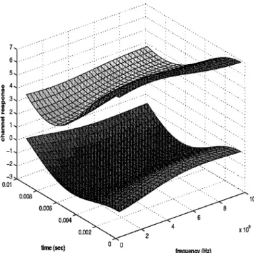
III. ESTIMATIONBASED ONREGRESSIONMODEL The discrete CR can be viewed as a sampled version of the 2-D continuous complex baseband fading process ; two typical examples of local , obtained by computer sim-ulation, are shown in Fig. 1. We first select an operating block in the time–frequency plane in which pilot symbols are uniformly inserted at every subchannel and every symbol; see Fig. 2. Then the receiver models the true sampled fading process in this region by a quadrature surface
(7) where represents the modeling error. For Rician or Rayleigh fading channels, is a complex Gaussian process, hence is also complex Gaussian-distributed. The frequency-domain model of the received samples (1) implies
Fig. 1. Two typical OFDM channel responses. They are plotted in the same figure for the convenience of comparison. The vertical coordinate does not represent the absolute magnitude of each CR surface.
Fig. 2. A typical pilot symbol distribution in the time–frequency plane of an OFDM signal.
that the ML estimates of the coefficients are chosen such that
is minimized, where is the estimator of in noise. The set in (8) contains the pilot locations in the oper-ating block (region)
(9)
Rewriting (7) as , where
, we restate the problem of finding the ML solution of (8) as solving
(10)
A. Algorithm Description
Taking the derivative of (10) with respect to and invoking the definitions
(11)
(12)
where is the complex conjugate of , we obtain the solution
(13)
Our final CR estimate, , for the position is
(14)
The above algorithm can be modified to estimate the CRs of either a single-carrier system or a subchannel of an OFDM system. This 1-D scheme models the fading process by a single-variable regression function, e.g., . The corresponding parameters are given by ,
and ,
respectively.
B. Complexity Analysis
Since all time–frequency blocks have the same size and pilot symbol distribution, if all the pilots are the same, the matrix
is fixed. Moreover, and are
real constant vectors. Computing the coefficient vector, , requires 2 6 real multiplica-tions and each requires 2 6 real
multiplica-tions. Hence, on the average, the number of real multiplications for each is
(15)
if the pilot density , being the
total number of (data plus pilot) symbols in a given block. In other words, less than four complex multiplications are needed for each estimate .
Note that enlarging the operating block size or the pilot den-sity increases only the summation terms in (13) [or (14)]; the average complexity (15) is not affected. For the LMMSE solu-tion, however, this means increasing the dimension of the corre-lation matrix in (5) and the complexity in matrix inverse opera-tion. Therefore, the operating region of the LMMSE algorithm is usually 1-D.
C. Estimation Error Analysis
A linear pilot-assisted channel estimate, including ours, has the form of (6), which can be expressed as
(16) where is the vector of noise terms in (4), ,
, and . is the error resulting from the interpolation process while is due to the presence of channel thermal noise.
For the proposed method, the variance of at , , is given by
(17) Assuming all pilot symbols are the same, i.e., , for all , we obtain the average (over positions) variance of
(18) where denotes the trace of the matrix . On the other hand, the interpolation error , which is independent of , is due to the modeling error in (7). Equation (18) does imply that, for fixed pilot density , can be reduced by
Fig. 3. BEP performance of the OFDM-16QAM system with the 2-D regression channel estimator;f T = 6:9 2 10 .
increasing ; however, so doing also leads to a larger op-erating block and hence larger . The situation becomes worse if Doppler frequency is large. On the other hand, we can cut back the modeling error by using a smaller operating block or a higher pilot density. Numerical examples supporting such conclusions are given in Section IV.
IV. NUMERICALRESULTS ANDDISCUSSION
Numerical examples obtained from computer simulations are provided in this section to demonstrate the effectiveness of the proposed CR estimate. We consider the multipath time-variant Rayleigh-fading channel based on (3), using ,
, and . All ’s are independent
stationary complex zero-mean Gaussian processes with unit variance while , 0.7305, 0.3175, 0.1137 and
, 0.1, 0.5, and 1 s, respectively.
Figs. 3 and 4 show the bit-error probability (BEP) perfor-mance of an OFDM-16QAM system whose 1-MHz bandwidth is divided into 32 subchannels. The effects of the Doppler shift and the 2-D pilot distribution are examined. As expected, with all other system parameters fixed, the error floor is an increasing function of the normalized Doppler frequency . Let denote the average SNR per bit. At lower ’s 30 dB when the BEP performance is dictated by the noise error [see (16)], the performance of our method is less sen-sitive to the pilot symbol density or number and is very close to that (curves labeled by perfect CE) of the theoretical lower bound obtained by assuming that CR is perfectly known. When is high, however, the modeling error dominates the system performance, hence the performance degrades for those esti-mates using a larger operating block or low-density pilots.
For comparison, we consider an estimator that uses the LMMSE method and then polynomial interpolation to ob-tain the data CRs in each subchannel. The performance of
Fig. 4. BEP performance of the OFDM-16QAM system with the 2-D regression channel estimator;f T = 4:16 2 10 .
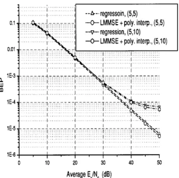
Fig. 5. BEP performance comparison for the LMMSE + polynomial-interpolation and 1-D regression estimators;f T = 2:76 2 10 .
this estimator is plotted in Figs. 5 and 6, assuming perfect knowledge about the channel correlation matrix and SNR. The performance of our algorithm (the 1-D regression estimator in this case) that has the same operating block size and pilot distribution is also shown in the same figure. It can be seen that both estimators yield very close BEP performance. The modeling error is an increasing function of the inter-pilot distance and becomes the limiting factor at high ’s. The issue of the worst-case pilot distribution is discussed in [7]. We show the worst-case behavior of both 1-D and 2-D estimators
Fig. 6. BEP performance comparison for the LMMSE + polynomial-interpolation and 1-D regression estimators;f T = 4:14 2 10 .
Fig. 7. BEP performance of the OFDM-16QAM system with the 1-D regression channel estimator;f = 80 Hz.
in Figs. 7 and 8. For the 2-D case, the system uses the same channel parameters as [7], i.e., 1024 subchannels and 5-MHz total bandwidth. As expected, the performance is improved as the pilot density increases. We also note that to meet a performance requirement a minimum pilot density must be in place.
Fig. 8. BEP performance of the OFDM-16QAM system with the 2-D regression channel estimator;f = 240 Hz except for the lowest curve which assumesf = 80 Hz.
V. CONCLUSION
We have proposed a new robust OFDM channel estimation scheme with excellent BEP performance. The proposed scheme is based on a nonlinear regression on the local time–frequency domain; it is of low complexity and does not need channel statis-tics or matrix inversion. Furthermore, with a proper pilot density, it achieves performance that is not far from the theoretical lower bound, and, within a wide range of , the performance of its 1-D version is very close to that of an LMMSE-based estimate.
REFERENCES
[1] J.-J. van de Beek, O. Edfors, M. Sandell, and S. K. Wilson, “On channel estimation in OFDM systems,” in Proc. 45th IEEE Vehicular Technology
Conf., Chicago, IL, July 1995, pp. 815–819.
[2] O. Edfors, M. Sandell, and J.-J. van de Beek, “OFDM channel estimation by sigular value decomposition,” IEEE Trans. Commun., vol. 46, pp. 931–939, July 1998.
[3] Y. (G.) Li et al., “Robust channel estimation for OFDM systems with rapid diversity fading channels,” IEEE Trans. Commun., vol. 46, pp. 902–915, July 1998.
[4] Y. Zhao and A. Huang, “A novel channel estimation method for OFDM mobile communication systems based on pilot signals and transform domain processing,” in Proc. IEEE 47th Vehicular Technology Confe., Phoenix, AZ, May 1997, pp. 2089–2093.
[5] M. Hsieh and C. Wei, “Channel estimation for OFDM systems based on comb-type pilot arrangement in frequency selective fading channels,”
IEEE Trans. Consumer Electron., vol. 46, pp. 931–939, July 1998.
[6] V. Mignone and A. Morello, “CD3-OFDM: A novel demodulation scheme for fixed and mobile receivers,” IEEE Trans. Commun., vol. 44, pp. 1144–1151, Sept. 1996.
[7] R. Nilson, O. Edfors, and M. Sandell, “An analysis of two-dimensional pilot-symbol assisted modulation for OFDM,” in Proc. IEEE Int. Conf.