應用於介面相符驗證之處理程序層級的功能涵蓋

全文

(1)應用於介面相符驗證之處理程序層級的功能涵蓋研究生 : 蘇曼勻. 指導教授 : 周景揚博士. 國立交通大學電子工程學系. 電子研究所碩士班. 摘要在設計現今的系統單晶片過程中，介面相符驗證扮演了一個相當重要的角色。一般而言，涵蓋量測有助於定量分析模擬式驗證的完整性；而在這篇論文中，我們針對介面相符驗證提出了處理程序層級的功能涵蓋方法，並發展一套可以在更高抽象層次描述處理程序的語言 – State-Oriented Language (SOL)。SOL 的表達能力較先前使用常規表示式的語言來的強，因此，藉由 SOL 便可在介面協定的規格有限狀態機模型上，更容易且不失嚴謹的詳細描述處理程序。經由實驗證明，我們所提議的方法的確可以有效的提高驗證的品質，並且加快驗證的效率。. i.

(2) Transaction-Level Functional Coverage for Interface Compliance Verification Student : Man-Yun Su. Advisor : Dr. Jing-Yang Jou. Department of Electronics Engineering Institute of Electronics National Chiao Tung University. ABSTRACT Interface compliance verification plays a very important role in modern SoC designs. In order to perform a quantitative analysis of simulation completeness, some coverage metrics are required. In this thesis, we propose a transaction-level functional coverage methodology for interface compliance verification. We also develop a new language, State-Oriented Language (SOL), to specify functional transactions at a higher level of abstraction. Moreover, SOL owns a stronger expressive power than previous regular-expression-based languages do. Therefore, by utilizing SOL, it is simple and rigorous to specify transactions from the specification FSM of the interface protocol. Experimental results show that the proposed methodology can effectively improve the verification quality and increase the verification efficiency.. ii.

(3) Acknowledgements I would like to express my sincere gratitude to my advisors, Professor Jing-Yang Jou and Professor Juinn-Dar Huang, for their insightful suggestion and patient guidance throughout the course of this work. I am also indebted to Che-Hua Shih, for his great help and constructive suggestions on my research. Special thanks to all members in the EDA lab for their friendship and company. Finally, I have to show my greatest appreciation to my family and my boyfriend, Wayne Hsieh. Without their love and encouragement, this work would not be completed.. iii.

(4) Contents 摘要 .................................................................................................................................. i ABSTRACT ...................................................................................................................... ii Acknowledgements ..........................................................................................................iii Contents ............................................................................................................................ iv List of Tables .................................................................................................................... vi List of Figures.................................................................................................................. vii Chapter 1 1.1 1.2. Introduction ................................................................................................... 1 Interface compliance verification .................................................................. 1 Coverage metrics ........................................................................................... 2 1.2.1 Code coverage ....................................................................................... 3 1.2.2 Functional coverage............................................................................... 5 1.3 Proposed approach......................................................................................... 6. Chapter 2 2.1 2.2 2.3. Transaction-Level Functional Coverage........................................................ 8 Related works ................................................................................................ 9 Motivation ................................................................................................... 12 Concept of our transaction description style ............................................... 13. Chapter 3 3.1. State-Oriented Language ............................................................................. 14 Abstract structure......................................................................................... 15. 3.2 3.3. Syntax conventions...................................................................................... 15 Boolean layer............................................................................................... 17 3.3.1 Extra signal qualification ( “ ” ) .......................................................... 17 3.4 Sequential layer ........................................................................................... 18 3.4.1 Concatenation ( ; ) ............................................................................... 18 3.4.2 Repetition ( [ ] ) ................................................................................... 19 3.4.3 Sequence AND ( && ) ........................................................................ 25. iv.

(5) 3.4.4 Sequence OR ( | ) ............................................................................... 26 3.4.5 Sequence fusion ( : ) ............................................................................ 27 3.5 Transaction layer ......................................................................................... 28 3.6 Coverage layer............................................................................................. 28 3.6.1 Sequence set cross ( ** ) ..................................................................... 29 3.7 Case study.................................................................................................... 30 Chapter 4. Proposed Methodology................................................................................ 36. Chapter 5 5.1 5.2. Experimental Results................................................................................... 38 Experimental environment .......................................................................... 38 Results analysis ........................................................................................... 41 5.2.1 Coverage comparison .......................................................................... 41 5.2.2 Efficiency improvement ...................................................................... 43. Chapter 6 6.1 6.2. Conclusions and Future Works.................................................................... 45 Contributions ............................................................................................... 46 Future works ................................................................................................ 46. References ....................................................................................................................... 48 Appendix A SOL Syntax Rule Summary ..................................................................... 51 Vita................................................................................................................................... 55. v.

(6) List of Tables Table 1. Design information. ........................................................................................... 39 Table 2. Coverage comparison for Case 1....................................................................... 42 Table 3. Coverage comparison for Case 2....................................................................... 43 Table 4. Efficiency improvement. ................................................................................... 44. vi.

(7) List of Figures Figure 1. The platform-based design methodology. .......................................................... 2 Figure 2. The interesting transactions derivation. ............................................................. 9 Figure 3. Sample transactions.......................................................................................... 11 Figure 4. CWL descriptions of Figure 3.......................................................................... 11 Figure 5. A 4-beat burst of the AMBA AHB protocol. .................................................... 12 Figure 6. An example FSM. ............................................................................................ 17 Figure 7. The spec. FSM of the simplified AMBA AHB slave protocol......................... 31 Figure 8. The flow of our verification methodology. ...................................................... 37 Figure 9. The experimental environment. ....................................................................... 39 Figure 10. The NEFSM of the AMBA AHB master........................................................ 40. vii.

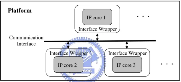
(8) Chapter 1 Introduction 1.1 Interface compliance verification In order to cope with the growing size and complexity of modern system-on-a-chip (SoC) designs, the block-based approach is used to partition the design into smaller blocks with well-defined functionality to be tackled by many individual teams. The blocks nowadays are usually reusable intellectual property (IP) cores, which are pre-designed and pre-verified, for the acceleration of the overall design process. To provide a higher level of reusability, the platform-based design methodology described in [1] is frequently adopted. Figure 1 illustrates the basic concept of this methodology. Since a system platform is based on a specific interface protocol, the used IP cores must be wrapped with appropriate interface logic before integration. If an IP core is desired in 1.

(9) another platform utilizing a different interface protocol, the designers only need to simply change the interface logic wrapper without altering the core inside. In this methodology, to ensure that each component can concordantly communicate with others within the system, it is very important to guarantee that the interface logic of each IP core conforms to the specific interface protocol before an SoC is built up. Hence, interface compliance verification becomes an essential part of the SoC verification flow.. Platform ‧‧‧. IP core 1 Interface Wrapper Communication Interface Interface Wrapper. Interface Wrapper. IP core 2. IP core 3. ‧‧‧. Figure 1. The platform-based design methodology.. 1.2 Coverage metrics Typically, the verification techniques can be classified into two types: formal methods and simulation-based ones. Formal verification is very efficient when verifying small designs. But it may take excessively long run time and suffer from memory explosion problem as the design size increases. Therefore, simulation is still the most commonly used method for design verification. During simulation, we can verify the functionality of a design in a short time by applying either direct (deterministic) or. 2.

(10) random patterns. Nevertheless, exhaustive simulation is nearly impossible for large designs. To notify us of how many of the verification patterns are enough and when the simulation can be done, an indicator is needed. Coverage metric is usually adopted as the indicator to perform a quantitative analysis of simulation completeness. Coverage metric means the method used to measure coverage. It usually comprises a lot of coverage tasks which are evaluated true when a specific condition is satisfied. By means of coverage metrics can not only objectively measure how well a design has been verified but also improve the quality of verification patterns. That is, it is capable of guiding either direct (deterministic) or random patterns to target those unverified design corners. As a result, coverage metrics can definitely provide a more systematic way to manage the simulation-based verification process. However, all of above hold only if suitable metrics are taken for different designs. Hence, exploring adequate coverage metrics is a very crucial issue in today’s functional verification. In general, there are two major categories of coverage metrics [2]: code coverage (structural coverage) and functional coverage.. 1.2.1 Code coverage Code coverage methods concentrate on identifying which part of the hardware description language (HDL) code has been executed in the design under verification (DUV). That is, they measure how much of the HDL implementation has been exercised. For example, statement coverage, branch (decision) coverage, expression (condition). 3.

(11) coverage, toggle coverage, and variable coverage are well-known code coverage metrics [3]. They are easy to define and measure. Once the definition is selected, the coverage metric can be derived from the HDL code intuitively. Besides, many commercial code coverage tools are available nowadays. However, the excitation of an erroneous statement does not necessarily mean that the incorrect value would manifest itself at an observation point during simulation. Activation without observation may not contribute to the error detection. Some approaches. are. proposed. to. address. this observability. issue.. In. [4],. the. observability-based code coverage metric (OCCOM) injects tags on each variable in the HDL code to simulate possible value changes caused by activated errors. Then it checks the percentage of tags that can be propagated to output ports. The validation vector grade (VVG) [5] extends toggle coverage by adding the concept of observability and arithmetic fault library. This approach is quite close to the gate level fault coverage. In [6], the extended condition coverage with excitation observation (ECC) detects the excitation of each condition variable and monitors the effect at output ports. In spite of these refinements, the fundamental issue of all code coverage metrics remains unchanged - they can only measure how well the structural HDL code has been exercised. They are not sufficient to represent the whole functionality of the design specification. Namely, the verification quality is generally considered not enough for modern complex SoC designs even if a high code coverage is achieved. Thus, the functional coverage is usually applied to further boost the verification quality.. 4.

(12) 1.2.2 Functional coverage Functional coverage, as its name implies, focuses on the design functionality. It measures how much of the original design specification has been exercised, and is independent of the HDL implementation details. In other words, when applying a given set of verification patterns, the function coverage results should be the same even if different HDL implementations are used for a specific design specification. Functional coverage includes item coverage and cross-product (cross) coverage. Item coverage concerns with a single specific attribute, which is sampled at specific locations at specific points in time with specific values. For example, a 4-beat burst and an 8-beat burst can be considered as two distinct items. Cross-product coverage is similar to item coverage. It consists of two or more items. For example, a 4-beat write burst can be a simple cross item while a 4-beat burst followed by an 8-beat one can be a complex cross item. Since the functional coverage metrics are specific to the design specification and application, they are considerably not straightforward to define and measure. Many methods are proposed to address these issues. In [7], a user defined cross-product coverage measurement tool is developed. [8] proposes a method for defining views on the cross-product functional coverage data. This method allows users to focus on the interesting information, and thus improve the quality of coverage analysis. In the cross-product functional coverage with LTL-assertions [9], auxiliary variables are used to reduce the number of assertions (coverage tasks) when collecting coverage information. The simulation overhead can thus be reduced. Some other works focus on. 5.

(13) the automation of the functional coverage metrics. In [10-11], the specification must be first given as a proprietary graph. Then the functional coverage analyzer can be automatically generated by traversing the graph. Although the methods mentioned above can facilitate interface compliance verification, the definitions or descriptions of the coverage metrics in [7-9] are still too complicated. It is not easy to put them to good use. Besides, the methods of the automatic generation of functional coverage metrics in [10-11] provide limited helps due to the proprietary graph is not generally used and designers may not be familiar with this form. Accordingly, these methods are hard to be widely used for the interface compliance verification.. 1.3 Proposed approach In this thesis, we propose a transaction-level functional coverage methodology, and provide a mean to specify functional transactions at a higher level of abstraction. First, the interface protocol is given as a specification FSM (spec. FSM) by using the concept in [12-13]. Then a transaction can be defined as a specific sequence of state transitions within the spec. FSM. We also develop a transaction description language, State-Oriented Language (SOL), which is cable of modeling diverse state transition sequences precisely and rigorously. The transactions can then be specified in a simpler and more systematic way. Moreover, the specified transactions with the spec. FSM can be translated into the corresponding functional coverage analyzer automatically. The rest of this thesis is organized as follows. In Section 2, the basic concept and. 6.

(14) the related works of transaction-level functional coverage are introduced. Section 3 presents the proposed new transaction description language State-Oriented Language. In Section 4, the details of our verification methodology are given. Section 5 demonstrates the proposed methodology with the AMBA AHB slave interface protocol and shows the experimental results. Finally, the concluding remarks are given in Section 6.. 7.

(15) Chapter 2 Transaction-Level Functional Coverage As mentioned, functional coverage concentrates on identifying how much of the original design specification has been verified, and it is favorable to improve the quality of interface compliance verification. Transaction-level functional coverage is one of the commonly used methods to measure the functional coverage for an interface design [14-16]. An interface protocol specification usually defines a set of different transactions. Note that a transaction here can be thought as the transfer of data and control over an interface to perform certain basic operation. For example, a transaction can be a 4-beat 8.

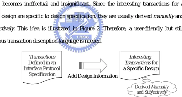
(16) burst or an 8-beat burst, or a 4-beat burst followed by an 8-beat one. By considering the design information (e.g., supported burst modes or responses) with these pre-defined transactions, the interesting transactions for a specific design can then be derived. Transaction-level functional coverage is generally measured by how many interesting transactions are exercised. However, a design instance usually implements a subset of the full interface protocol. For example, ‘WAIT’ response is optional in a specific interface protocol. A design which complies with this interface protocol does not allow ‘WAIT’ response during transaction. If ‘WAIT’ response is required to occur in coverage metric for this design, the coverage will never achieve 100%. This coverage result becomes ineffectual and insignificant. Since the interesting transactions for a given design are specific to design specification, they are usually derived manually and subjectively. This idea is illustrated in Figure 2. Therefore, a user-friendly but still rigorous transaction description language is needed. Transactions Defined in an Interface Protocol Specification. Interesting Transactions for a Specific Design Add Design Information Derived Manually and Subjectively. Figure 2. The interesting transactions derivation.. 2.1 Related works Several approaches are proposed for transaction-level functional coverage. For M-path coverage [13], the protocol is first modeled as a spec. FSM. Then an M-path is defined as a path which can form a complete bus transfer in the FSM model. In other 9.

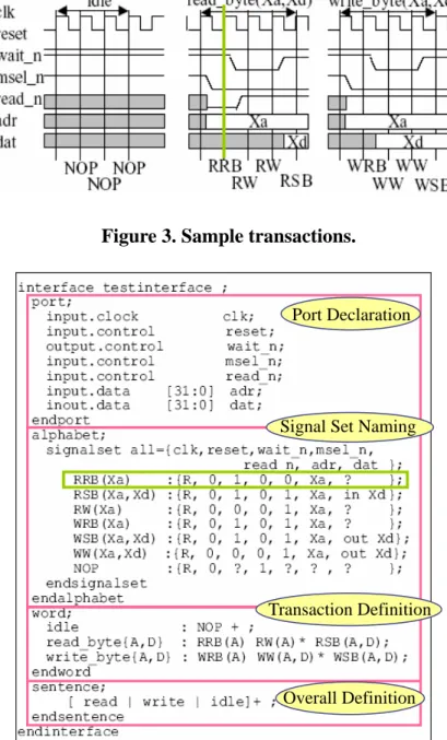
(17) words, an M-path, which is a finite sequence of state transitions, is actually a simple transaction. M-paths are used as the targets for coverage measurement. However, the proposed FSM model here is too simple. Since only several control signals are checked, many transactions cannot be differentiated from others. For the AMBA AHB protocol, the write transactions cannot be distinguished from the read ones due to the signal HWRITE is not checked. This may make it too easy to achieve 100% M-path coverage. Besides, the definition of M-path is neither clear nor rigorous enough. It is not convenient to put it to good use for lack of sufficient expressive power. Moreover, consecutive transfers are not considered in this work. It may conceal the design errors since some errors may merely occur during consecutive transfers. In [14], Component Wrapper Language (CWL) is used to describe signal sequences based on regular expressions. For example, there are three sample transactions, idle, read and write. The timing diagram of each transaction is given in Figure 3. CWL descriptions of these transactions are depicted in Figure 4. In CWL descriptions, the input and output signals must be declared first. Then signal values at each cycle are defined as signal sets. For the cycle RRB, the signal values of clk, reset, wait_n, msel_n, read_n, adr, and dat are R (for rising edge), 0, 1, 0, 0, Xa (for the read address), and ? (for the unknown read data), respectively. Next, each simple transaction is modeled by utilizing the defined signal sets. For example, the idle transaction comprises at least one NOP. Finally, a more complex transaction can be built up by assembling simple ones. Users can construct transactions and do transaction-level verification by using CWL.. 10.

(18) idle. read. write. Figure 3. Sample transactions.. Port Declaration. Signal Set Naming. Transaction Definition. Overall Definition. Figure 4. CWL descriptions of Figure 3. In this approach, individual signals need to be considered when describing thorough transactions. In other words, the signal-level descriptions are required. If the transactions are getting more complex, it might be troublesome and time-consuming to. 11.

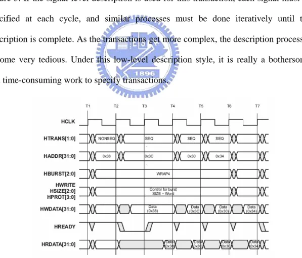
(19) author the corresponding CWL descriptions. Thus, CWL is not suitable to model complex transactions.. 2.2 Motivation Typically, the interesting transactions need to be derived manually before measuring transaction-level functional coverage. It is tedious and error-prone for human to specify transactions if the detailed signal values are required. Take a 4-beat burst of the AMBA AHB protocol as an example. The corresponding timing diagram is given in Figure 5. If the signal-level description is used for this transaction, each signal must be specified at each cycle, and similar processes must be done iteratively until the description is complete. As the transactions get more complex, the description processes become very tedious. Under this low-level description style, it is really a bothersome and time-consuming work to specify transactions.. Figure 5. A 4-beat burst of the AMBA AHB protocol.. 12.

(20) To cope with this issue, it is a good idea to provide a simple, human-friendly, rigorous, and systematic way to specify transactions at a higher level of abstraction instead of at the signal level.. 2.3 Concept of our transaction description style The transaction description style in our approach is directly inspired by the work proposed in [12-13]. Both works give the concept of specifying interface protocol in the higher FSM level. All engineers are very familiar with this style and are very likely to accept this style since no particular specification languages need to be learned. In our work, the interface protocol is specified as a spec. FSM by using the methods in [12-13]. The spec. FSM only needs to be created once for a specific interface protocol and can be massively reused later. A transaction can then be defined as a specific sequence of state transitions within the spec. FSM. This enables the use of states in the spec. FSM as basic elements to describe transactions. This method can raise the level of abstraction as well as encapsulate the details of the low-level signals. In other words, the detailed signal values are no longer required. Hence, one can put more emphasis on the functionality at the higher FSM level.. 13.

(21) Chapter 3 State-Oriented Language Since the existing transaction description languages are neither simple nor human-friendly enough, we develop a new transaction description language, State-Oriented Language (SOL), in which we can specify transactions at the higher FSM level. In SOL, PSL-like syntax [17] is used to represent a sequence of state transitions within the spec. FSM as a transaction. We believe the expressive power of SOL is stronger than that of traditional regular-expression-based approaches. Therefore, it is easier to model complex transactions by using SOL.. 14.

(22) 3.1 Abstract structure SOL consists of four layers - Boolean, Sequential, Transaction, and Coverage layer - which cut the language along the axis of functionality. (1) Boolean layer is used to build expressions which are used by the other layers. Boolean expressions are evaluated over a single state transition. (2) Sequential layer is used to describe basic sequences. Sequential expressions are evaluated over a specific sequence of state transitions. (3) Transaction layer is used to define sequences as transactions (named sequences) by using the assignment operator. (4) Coverage layer is used to specify interesting transactions for coverage measurement.. 3.2 Syntax conventions The formal syntax described in this work uses the following extended Backus-Naur Form (BNF). (1) The initial character of each word in a nonterminal is capitalized. A nonterminal can be either a single word or multiple words separated by underscores. When a multiple-word nonterminal containing underscores is referred within the text, the underscores are replaced with spaces. For example, Boolean_Expression Indicates a Boolean Expression.. 15.

(23) (2) Boldface words are used to denote reserved keywords, operators, and punctuation marks as a required part of the syntax. These words appear in a larger font for distinction. For example,. “Condition” (3) The ::= operator separates the two parts of a BNF syntax definition. The syntax category appears to the left of this operator and the syntax description appears to the right of the operator. For example, Condition ::= Boolean_Expression (4) A vertical bar separates alternative items (use one only) unless it appears in boldface, in which case it stands for itself. For example, SERE ::= State | Sequence | Sequence_Name (5) Square brackets enclose optional items unless they appear in boldface. In which case they stand for themselves. For example, State ::= State [“Condition”] Indicates “Condition” is an optional syntax item for State. (6) Braces enclose a repeated item unless they appear in boldface, in which case they stand for themselves. A repeated item may appear zero or more times. For example, Sequence_Set ::= < {Sequence_Name} { ,{Sequence_Name} } > Indicates {Sequence_Name} may appear more than one time. (7) A comment is preceded by a colon unless it appears in boldface, in which case it stands for itself.. 16.

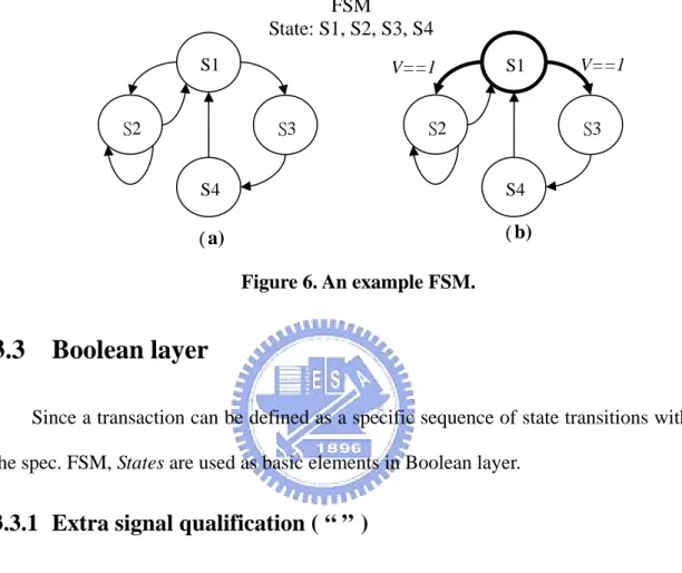
(24) The detailed syntax of SOL is introduced below (shown in shaded area). The FSM shown in Figure 6 is taken as an example to introduce the operators in SOL. FSM State: S1, S2, S3, S4 S1 S2. V==1. S1. S2. S3. V==1 S3. S4. S4. (a). (b) Figure 6. An example FSM.. 3.3 Boolean layer Since a transaction can be defined as a specific sequence of state transitions within the spec. FSM, States are used as basic elements in Boolean layer.. 3.3.1 Extra signal qualification ( “ ” ) In order to keep the spec. FSM as simple as possible, extra signals can be included in additional to the states while defining a transaction. The Boolean expression built from the extra signals should be enclosed in double quotes, shown in Box 1.. State ::= State [ “Condition” ] Condition ::= Boolean_Expression : An expression that yields a logical value. Box 1. Extra signal qualification.. 17.

(25) Example 1. In Figure 6(b), the extra signal V must be checked to be true when moving from S1 to the next state. S1 “ V==1 ”. 3.4 Sequential layer State Extended Regular Expressions (SEREs), shown in Box 2, describe single-cycle or multi-cycle behavior built from a series of States. SERE ::= State | Sequence | Sequence_Name Sequence ::=. { SERE } Box 2. SEREs and Sequences.. 3.4.1 Concatenation ( ; ) The concatenation operator, shown in Box 3, constructs a SERE that is the concatenation of two other SEREs. SERE ::= SERE. ;. SERE. Box 3. Concatenation operator.. 18.

(26) Example 2. In Figure 6(a), T1 is a transaction with the state transitions that starts from S1, then moves through S3, S4, and ends at S1. T1 : S1 Æ S3 Æ S4 Æ S1 T1 = { S1 ; S3 ; S4 ; S1 }; The sequence can be defined as a transaction by using the assignment operator which is detailed described in Section 3.5 Transaction layer. Example 3. In Figure 6(b), T2 is another transaction with the same state transitions sequence as T1 while the extra signal V must be true when moving from S1 to S3. V == 1. T2 : S1 ⎯⎯⎯→ S3 Æ S4 Æ S1 T2 = { S1 “V == 1” ; S3 ; S4 ; S1 };. 3.4.2 Repetition ( [ ] ) The repetition operators are used to describe succinctly repeated concatenations of a sequence. There are three types of repetition operators: consecutive repetition ( [* ] ), non-consecutive repetition ( [= ] ), and goto repetition ( [Æ ] ). Each is introduced below.. 19.

(27) (a) consecutive repetition ( [* ] ) The consecutive repetition operator, shown in Box 4, constructs repeated concatenation of the same State or Sequence. SERE ::= State |. Sequence. |. State. | Count ::=. Sequence. [* [Count] ] [* [Count] ] [+] [+]. Non-negative integer | Range Range ::= Low_Bound : High_Bound Low_Bound ::= Non-negative integer | 0 High_Bound ::= Non-negative integer | inf. Box 4. Consecutive repetition operator. Informal semantics: A[*n] A[*n:m] A[*:m] = A[*0:m] A[*n:] = A[*n:inf] A[*] = A[*:] = A[*0:inf] A[+] = A[*1:]. (0 ≦ n ≦ m) A repeats n times A repeats between n to m times A repeats at most m times (including 0 time) A repeats at least n times A repeats any number of times (including 0 time) A repeats at least one time. 20.

(28) Example 4. In Figure 6(a), T3 is a transaction with the state transitions that starts from S1, moves to S2, and stays at S2 for three consecutive cycles, then ends at S1. T3 : S1 Æ S2 Æ S2 Æ S2 Æ S1 T3 = { S1 ; S2 ; S2 ; S2 ; S1 }; T3 can also be defined by using the consecutive repetition operator. T3 = { S1 ; S2[*3] ; S1 }; Example 5. In Figure 6(a), T4 is a transaction with the state transitions that starts from S1, moves to S2, and stays at S2 for one to five consecutive cycles, then ends at S1. T4 : S1 Æ S2 (1~5 cycles) Æ S1 T4 = { S1 ; S2[*1:5] ; S1 }; Example 6. In Figure 6(a), T5 is a transaction with the state transitions that starts from S1, moves to S2, and stays at S2 for any consecutive cycles (including zero cycle). T5 : S1 Æ S2 (Any number of cycle) T5 = { S1 ; S2[*] };. 21.

(29) (b) non-consecutive repetition ( [= ] ) The non-consecutive repetition operator, shown in Box 5, constructs repeated (possibly non-consecutive) concatenation of a State.. SERE ::= State [= Count ] Count ::= Non-negative integer | Range Range ::= Low_Bound : High_Bound Low_Bound ::= Non-negative integer | 0 High_Bound ::= Non-negative integer | inf. Box 5. Non-consecutive repetition operator. Informal semantics: A[=n] A[=n:m] A[=:m] = A[=0:m] A[=n:] = A[=n:inf] A[=:] = A[=0:inf]. (0 ≦ n ≦ m) A occurs n times A occurs between n to m times A occurs at most m times (including 0 time) A occurs at least n times A occurs any number of times (including 0 time). Example 7. In Figure 6(a), T6 is a transaction with the state transitions that starts from S1, and then visits S2 three times. The visits of S2 need not to be in consecutive cycles. In addition, T6 holds after the 3rd S2 is visited and still holds before the 4th S2 appears.. 22.

(30) T6 : S1 Æ…Æ S2 Æ…Æ S2 Æ…Æ S2 Æ… T6 = { S1 ; S2[=3] }; If the transactions below occur during simulation, T6 matches from the state S1 to the state before the 4th S2 happened. S1ÆS2ÆS2ÆS2ÆS1ÆS3ÆS4ÆS1ÆS2 S1ÆS2ÆS1ÆS2ÆS1ÆS2ÆS1ÆS2 S1ÆS3ÆS4ÆS1ÆS2ÆS2ÆS2ÆS2 S1ÆS3ÆS4ÆS1ÆS2ÆS2ÆS1ÆS3ÆS4ÆS1ÆS2ÆS2. (c) goto repetition ( [Æ ] ) The goto repetition operator, shown in Box 6, constructs repeated (possibly non-consecutive) concatenation of a State, such that it holds on the last cycle of the sequence.. SERE ::= State [Æ [Positive_Count] ] Positive_Count ::= Positive integer | Positive_Range Positive_Range ::= Low_Bound : High_Bound Low_Bound ::= Positive integer | 1 High_Bound ::= Positive integer | inf. Box 6. Goto repetition operator.. 23.

(31) Informal semantics: A[Æn] A[Æn:m] A[Æ:m] = A[Æ1:m] A[Æn:inf] = A[Æn:] A[Æ1:inf] = A[Æ:] A[Æ] = A[Æ1]. (1 ≦ n ≦ m) A occurs n times A occurs between n to m times A occurs at most m times (excluding 0 time) A occurs at least n times A occurs one or more times A occurs exactly one time. Example 8. In Figure 6(a), similar to T6, T7 is also a transaction with the state transitions starts from S1, then moves to S2 three times (can be non-consecutive). In addition, T7 holds only at the cycle in which the 3rd S2 is visited. T7 : S1Æ…Æ S2 Æ…Æ S2 Æ…Æ S2 T7 = { S1 ; S2[Æ3] }; Under the same condition during simulation as that in Example 7, T7 matches from the state S1 to the 3rd S2 exactly. S1ÆS2ÆS2ÆS2ÆS1ÆS3ÆS4ÆS1ÆS2 S1ÆS2ÆS1ÆS2ÆS1ÆS2ÆS1ÆS2 S1ÆS3ÆS4ÆS1ÆS2ÆS2ÆS2ÆS2 S1ÆS3ÆS4ÆS1ÆS2ÆS2ÆS1ÆS3ÆS4ÆS1ÆS2ÆS2. 24.

(32) 3.4.3 Sequence AND ( && ) The transaction comprising two sequences using the sequence AND operator, shown in Box 7, holds only if both sequences hold and complete at the same cycle. SERE ::= Sequence && Sequence Sequence ::=. { SERE } Box 7. Sequence AND operator. Example 9. In Figure 6(a), similar to T7, T8 is also a transaction with the state transitions starts from S1, and then visit S2 three times (can be non-consecutive). However, S3 is strictly not allowed showing up in the sequence T7. T8 : S1 Æ…(!S3) Æ S2 Æ…(!S3) Æ S2 Æ…(!S3) Æ S2 T8 = { S1 ; {S3[=0]} && {S2[Æ3]} }; Under the same simulation condition as that in Example 8, T8 not only matches to the 3rd S2 exactly but the state S3 occurs zero time within the matched duration. S1ÆS2ÆS2ÆS2ÆS1ÆS3ÆS4ÆS1ÆS2 S1ÆS2ÆS1ÆS2ÆS1ÆS2ÆS1ÆS2 S1ÆS3ÆS4ÆS1ÆS2ÆS2ÆS2ÆS2 S1ÆS3ÆS4ÆS1ÆS2ÆS2ÆS1ÆS3ÆS4ÆS1ÆS2ÆS2. 25.

(33) 3.4.4 Sequence OR ( | ) The transaction comprising two sequences using the sequence OR operator, shown in Box 8, holds if one of two alternative sequences holds. SERE ::= Sequence. |. Sequence. Sequence ::=. { SERE } Box 8. Sequence OR operator. Example 10. In Figure 6(a), T9 is either one of the following two sequences, T9 :. S1 Æ S3 Æ S4 Æ S1 S1 Æ S2 Æ S2 Æ S2 Æ S1. T9 = { {S1;S3;S4;S1} | {S1;S2[*3];S1} }; Note that above two sequences are previously defined as T1 and T3. Hence, T9 can also be defined in terms of these named sequences. T9 = { {T1} | {T3} }; Under the same simulation condition as before, T9 matches sequence T1 or T3. S1ÆS2ÆS2ÆS2ÆS1ÆS3ÆS4ÆS1ÆS2 S1ÆS2ÆS1ÆS2ÆS1ÆS2ÆS1ÆS2 S1ÆS3ÆS4ÆS1ÆS2ÆS2ÆS2ÆS2 S1ÆS3ÆS4ÆS1ÆS2ÆS2ÆS1ÆS3ÆS4ÆS1ÆS2ÆS2. 26.

(34) 3.4.5 Sequence fusion ( : ) Similar to the concatenation operator, the sequence fusion operator, shown in Box 9, concatenates two sequences overlapping by one cycle. In other words, the 2nd sequence starts at the cycle in which the 1st sequence completes. This operator is used to concatenate two consecutive transactions. SERE ::= Sequence. :. Sequence. Sequence ::=. { SERE } Box 9. Sequence fusion operator. Example 11. In Figure 6(a), T10 is a transaction shown below, T10 : S1ÆS3ÆS4ÆS1ÆS2ÆS2ÆS2ÆS1 T10 = { S1;S3;S4;S1;S2[*3];S1 }; T10 can also be treated as two sequences that overlap each other for one cycle: T10 : S1ÆS3ÆS4ÆS1 : S1ÆS2ÆS2ÆS2ÆS1 T10 = { {S1;S3;S4;S1} : {S1;S2[*3];S1} }; Again, T10 can also be defined in terms of T1 and T3. T10 = { {T1} : {T3} };. 27.

(35) 3.5 Transaction layer A sequence can be defined once as a named sequence (transaction) and then be reused later. The assignment operator, shown in Box 10, is used to declare a named sequence. The left-hand side of the assignment operator becomes a synonym for the sequence on the right-hand side. The sequence names must be enclosed in braces when referred. This operator is extensively used in the previous examples. Transaction_Declaration ::= Sequence_Name = Sequence ;. Box 10. Transaction declaration.. 3.6 Coverage layer The interesting transactions for coverage measurement, shown in Box 11, can be defined by the previously declared sequence names or generated by the sequence set cross operator. Coverage_Declaration ::= Sequence_Name ; |. Sequence_Cross ;. Box 11. Coverage declaration.. 28.

(36) 3.6.1 Sequence set cross ( ** ) A sequence set comprises one or more sequences. Sequences are enclosed in angle bracket and separated by commas. A sequence set cross operator, shown in Box 12, is used to represent a set of back-to-back consecutive transactions with cross behavior. Sequence_Cross ::= Sequence_Set ** Sequence_Set { ** Sequence_Set } Sequence_Set ::=. < {Sequence_Name} { ,{Sequence_Name} } > Box 12. Sequence set cross operator. Example 12. Assume the transactions with the following cross behavior are interesting. T1. T3 T4. T2. T5. These 6 transactions can be defined by the previously introduced operator: {{T1}:{T3}};. {{T1}:{T4}};. {{T1}:{T5}};. {{T2}:{T3}};. {{T2}:{T4}};. {{T2}:{T5}};. These transactions can also be defined by using the sequence set cross operator. The transaction T1 and T2 can form a sequence set, and the transaction T3, T4, and T5 can form another. Then these 6 transactions can be defined as follows, <{T1},{T2}> ** <{T3},{T4},{T5}>;. 29.

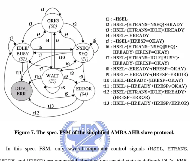
(37) This means each sequence in the first sequence set must be followed by each sequence in the next sequence set, respectively. Example 13. The sequence set cross operator can also work on more than two sequence sets. <{T1},{T2}> ** <{T3},{T4}> ** <{T9},{T10}>; For this expression, 8 (2*2*2) transactions are generated for coverage measurement. That is, {{T1}:{T3}:{T9}}; {{T1}:{T3}:{T10}}; {{T1}:{T4}:{T9}}; {{T1}:{T4}:{T10}}; {{T2}:{T3}:{T9}}; {{T2}:{T3}:{T10}}; {{T2}:{T4}:{T9}}; {{T2}:{T4}:{T10}};. The sequence set cross operator can provide a much more elegant but equivalent representations while the transactions become complex. This operator can reduce the transaction description complexity as well as help generate more interesting transactions easily.. 3.7 Case study To apply our methodology, the interface protocol should be given as a spec. FSM first. The details about how to construct a spec. FSM can be found in [12-13]. The AMBA AHB slave interface protocol [18] is adopted as an example here to demonstrate how to define transactions in SOL. The spec. FSM of the simplified AMBA AHB slave protocol is given in Figure 7. 30.

(38) Figure 7. The spec. FSM of the simplified AMBA AHB slave protocol. In this spec. FSM, only several important control signals (HSEL, HTRANS, HREADY, and HRESP) are concerned. Besides, one special state is defined: DUV_ERR. If the DUV behaves illegally, the design moves to the state DUV_ERR. Otherwise, the design moves among the other normal states excluding DUV_ERR. By traversing the spec. FSM, many defined properties can be found. For example, in the state IDLE/BUSY, if HREADY is not asserted or HRESP is not set to OKAY, the design moves to the state DUV_ERR. This infers that a slave cannot respond anything but a zero WAIT state OKAY response to an IDLE or a BUSY transfer. In addition, in the state WAIT, if HREADY is asserted but HRESP is not set to OKAY, the design moves to the state DUV_ERR. This implies that a slave can only respond OKAY when HREADY is transient to be asserted. These are explicitly defined in the AMBA AHB specification.. 31.

(39) However, the spec. FSM is not omnipotent for the lack of consideration to each signal. For example, the read transactions cannot be distinguished from the write transactions. The burst mode of each transaction cannot be detected, either. To retrieve these issues, the extra signal qualification operation should be applied. Now, use SOL to define basic transactions on the spec. FSM. Example 1. A 1-beat burst transaction. The construction procedure of a 1-beat burst transaction can be decomposed into four steps. (1) For a 1-beat burst transaction, the signal HBURST must be set to 0. (2) The given design must move to state NSEQ/SEQ (S1) one time and cannot move to state ERROR (S4) for a complete 1-beat transfer, i.e.,. {S4[=0]} && {S1[Æ1]} .. (3) A 1-beat burst transaction consists of two cases. One starts from the state ORIG (S0), which indicates the slave is just selected and going to do the first transaction. The other starts from the state NSEQ/SEQ (S1), which implies the slave is already selected and going to do another transaction. 1 starting from the state ORIG (S0) : ○. OneBeat_S0 = {S0 “HBURST==0”;{S4[=0]}&&{S1[Æ1]}}; 2 starting from the state NSEQ/SEQ (S1) : ○. OneBeat_S1 = {S1 “HBURST==0”;{S4[=0]}&&{S1[Æ1]}}; 32.

(40) (4) A 1-beat burst transaction is either the sequence OneBeat_S0 or the sequence OneBeat_S1. Then a 1-beat burst transaction is composed of these two sequences by using the sequence OR operator. That is, OneBeat = {{OneBeat_S0} | {OneBeat_S1}}; Example 2. A 4-beat burst transaction. The construction procedure of a 4-beat burst transaction is similar to that of a 1-beat burst transaction. (1) The signal HBURST should be set to 2 or 3. (2) The design must visit the state NSEQ/SEQ (S1) four times and cannot move to state ERROR (S4) to complete a 4-beat transfer, i.e., {S4[=0]} && S1[Æ4] . (3) A 4-beat burst transaction also consists of two cases. 1 starting from the state ORIG (S0) : ○. FourBeat_S0 = {S0 “HBURST==2 || HBURST==3”;{S4[=0]}&&{S1[Æ4]}}; 2 starting from the state NSEQ/SEQ (S1) : ○. FourBeat_S1 = {S1 “HBURST==2 || HBURST==3”;{S4[=0]}&&{S1[Æ4]}}; (4) A 4-beat burst transaction can then be defined as, FourBeat = {{FourBeat_S0} | {FourBeat_S1}};. 33.

(41) Follow similar procedure, more basic transactions can be defined. For a 4-beat burst with wait transaction (FourBeatWithWAIT), the state WAIT (S3) must be visited at least one time during the transaction. That is, the sequence {S3[=1:]} must hold. Therefore, the 2nd step of the construction procedure of the 4-beat burst with wait transaction must be written as {S3[=1:]}&&{{S4[=0]}&&{S1[Æ4]}}. For an 8-beat write burst transaction (EightBeatWrite), the signal HBURST must be set to proper values (4 or 5) and the signal HWRITE must be asserted, i.e., the 1st step: (HBURST==4 || HBURST==5) && HWRITE . As well, the design must visit the state NSEQ/SEQ (S1) eight times during this 8-beat burst transaction, i.e., the 2nd step: {S4[=0]} && {S1[Æ8]}. Example 3. A 4-beat burst transaction instantly followed by an 8-beat write burst transaction. A 4-beat burst transaction (FourBeat) and an 8-beat write burst transaction (EightBeatWrite) are defined before. Since the required transaction can be defined by fusing these two transactions, it can be written as follows, {{FourBeat}:{EightBeatWrite}};. More complex transactions can be constructed by the sequence fusion operator ( : ). For example, a 1-beat burst transaction followed by an 8-beat write burst transaction, then followed by a 4-beat burst transaction can be defined as follows, {{OneBeat}:{EightBeatWrite}:{FourBeat}}; 34.

(42) In addition, the sequence set cross operator ( ** ) can be used to describe a lot of back-to-back consecutive transactions in a more easy way. The expression below can represent 12 (3*2*2) different consecutive transactions. <{EightBeatWrite},{FourBeatWithWAIT},{OneBeat}> ** <{FourBeat},{OneBeat}> ** <{EightBeatWrite},{FourBeat}>; If the interesting transactions are comprised by many other transactions with this complex cross behavior, the sequence set cross operator can provide a strong expressive power.. 35.

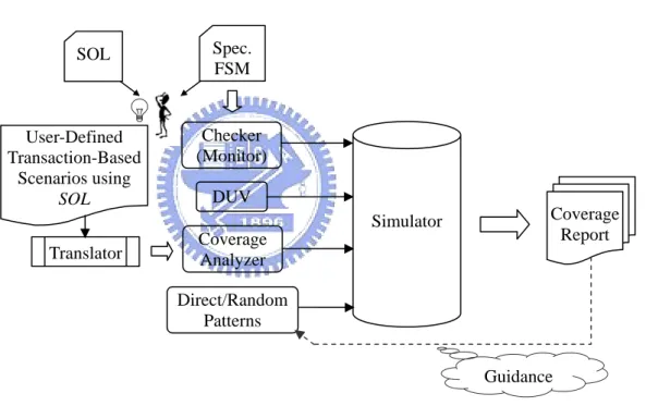
(43) Chapter 4 Proposed Methodology By means of SOL, transactions can be defined in a simpler, but still rigorous, and more systematic way. As well, the transaction-level functional coverage for the interface compliance verification can be done at the higher FSM level. The flow of our verification methodology is illustrated in Figure 8. The interface protocol needs to be first specified as a spec. FSM by using the methods in [12-13]. Note that the spec. FSM can be translated into an interface protocol checker [13]. Meanwhile, a transaction can be thought as a specific sequence of state transitions within the spec. FSM. The interesting transactions are manually specified by using SOL. These transactions with the spec. FSM are further translated into a functional coverage 36.

(44) analyzer automatically. Next, we simulate the whole system, including the DUV, verification patterns, checker, and coverage analyzer. According to the outcome of the checker, we can know if the DUV conforms to the interface protocol. From the coverage analyzer, the report tells how many interesting transactions have been verified. Moreover, the coverage information can guide either direct or random patterns to hit those unverified design corner cases.. SOL. User-Defined Transaction-Based Scenarios using SOL. Spec. FSM. Checker (Monitor) DUV Coverage Report. Simulator Translator. Coverage Analyzer Direct/Random Patterns. Guidance. Figure 8. The flow of our verification methodology.. 37.

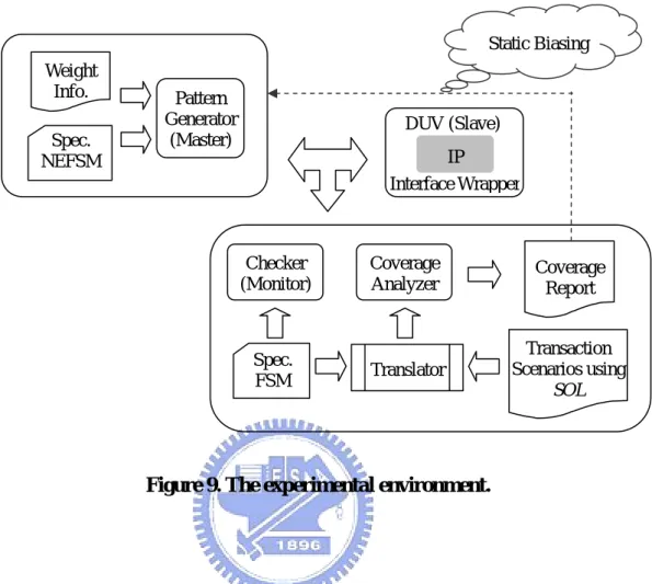
(45) Chapter 5 Experimental Results 5.1 Experimental environment To demonstrate our methodology, we choose the AMBA AHB slave interface protocol [18] as an example. The spec. FSM of simplified AMBA AHB slave protocol is given in Figure 7. Figure 9 illustrates the experimental environment. It consists of three parts: a DUV, a constraint-driven random pattern generator, and the proposed work.. 38.

(46) Static Biasing Weight Info. Spec. NEFSM. Pattern Generator (Master). DUV (Slave) IP Interface Wrapper. Checker (Monitor). Coverage Analyzer. Coverage Report. Spec. FSM. Translator. Transaction Scenarios using SOL. Figure 9. The experimental environment.. (1) The DUV is the slave which we want to verify. The experiments are conducted over three real AHB slave designs. The information about these three designs is shown in Table 1. The design RGB2YCrCB is a RGB-to-YCrCB color space converter. The design MAC is a multiply-accumulator. The design Convolution is a convolution calculator for discrete wavelet transfer. Table 1. Design information. Design RGB2YCrCb MAC Convolution. Supporting AHB responses OKAY OKAY, ERROR OKAY (wait). 39. # of State / Transition / M-path 3 / 8 / 14 4 / 10 / 12 4 / 10 / 16.

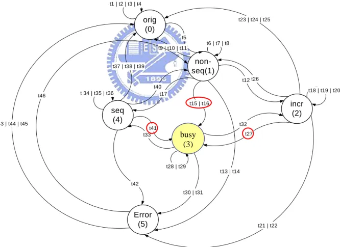
(47) (2) The constraint-driven random pattern generator is an AHB master which generates verification patterns based on an NEFSM (Non-deterministic Extended FSM) with the weight information about the transitions and bursts. The NEFSM is given in Figure 10. The weight of each transition and burst is configurable. For example, the weights of transition t15, t16, t27, and t41 can be assigned to a higher value to increase the probability of the occurrence of BUSY conditions. In order to balance the occurrence of total verification patterns, the transitions and bursts are assigned to be equal weight. t1 | t2 | t3 | t4. orig (0). t23 | t24 | t25. t5 t6 | t7 | t8 t9 | t10 | t11. nonseq(1). t37 | t38 | t39. t12 t26 t46. t40 t17. t 34 | t35 | t36. t18 | t19 | t20. incr (2). t15 | t16. t43 | t44 | t45. seq (4) t41 t33. t32. busy busy (3). t27. t28 | t29 t13 | t14. t42 t30 | t31. Error (5). t21 | t22. Figure 10. The NEFSM of the AMBA AHB master.. 40.

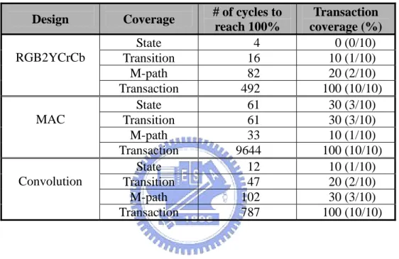
(48) (3) We develop a translator which accepts the spec. FSM and user-defined SOL transactions then produces the corresponding coverage analyzer. The coverage report tells how many interesting transactions have been verified. In addition, the coverage information is used to help statically bias the random pattern generator to create more effective verification patterns.. 5.2 Results analysis Two experiments are conducted: coverage comparison and efficiency improvement. In the first experiment, four coverage results (State coverage, Transition coverage, M-path coverage, and our Transaction coverage) are compared for three designs, respectively. In the second experiment, the coverage information is sent back to bias the random pattern generator to produce more effective patterns.. 5.2.1 Coverage comparison Case 1 The interesting transactions are defined as 10 basic read and write transactions as follows, {IncrBeatRead};. {OneBeatRead};. {FourBeatRead};. {EightBeatRead};. {SixteenBeatRead};. {IncrBeatWrite};. {OneBeatWrite};. {FourBeatWrite};. {EightBeatWrite};. {SixteenBeatWrite};. The comparison results are shown in Table 2. Since the supporting responses of each design are different from each other, each takes distinct simulation time to reach 100% State/Transition/M-path/Transaction coverage. For the design RGB2YCrCb, it takes 4/16/82/492 cycles to reach 100% State/Transition/M-path/Transaction coverage.. 41.

(49) As the State/Transition/M-path coverage reach 100%, the Transaction coverage is only 0/10/20%. For the other two designs, the results are similar. It is observed that the Transaction coverage is very low while the other three coverage metrics reach 100%. Table 2. Coverage comparison for Case 1. Design RGB2YCrCb. MAC. Convolution. # of cycles to reach 100% 4 16 82 492 61 61 33 9644 12 47 102 787. Coverage State Transition M-path Transaction State Transition M-path Transaction State Transition M-path Transaction. Transaction coverage (%) 0 (0/10) 10 (1/10) 20 (2/10) 100 (10/10) 30 (3/10) 30 (3/10) 10 (1/10) 100 (10/10) 10 (1/10) 20 (2/10) 30 (3/10) 100 (10/10). Case 2 Make the interesting transactions more complex by adding 15 more basic transactions with BUSY or WAIT (e.g, {OneBeatWithWAIT}; {FourBeatWithBUSY}; {FourBeatWithWAIT}; {EightBeatWithBUSY};, etc.) and 25 back-to-back consecutive transactions (i.e., <{IncrBeat},{OneBeat},{FourBeat},{EightBeat},{SixteenBeat}>** <{IncrBeat}, {OneBeat},{FourBeat},{EightBeat},{SixteenBeat}>;). The comparison results are shown in Table 3. Since the status of the random pattern generator is the same as that in Case 1, the design Convolution still takes 12/47/102. 42.

(50) cycles to reach 100% State/Transition/M-path coverage. But it takes 11135 cycles to reach 100% Transaction coverage. As the State/Transition/M-path coverage reach 100%, the Transaction coverage is only 4/8/12%. It is shown that the Transaction coverage is even lower than that in Case 1 as the other three coverage metrics reach 100%. Table 3. Coverage comparison for Case 2. Design Convolution. # of cycles to reach 100% 12 47 102 11135. Coverage State Transition M-path Transaction. Transaction coverage (%) 4 (2/50) 8 (4/50) 12 (6/50) 100 (50/50). From these two cases, we get some conclusions. While the interesting transactions become more complex, it needs a significantly longer simulation time to reach 100% Transaction coverage. Besides, as the State/Transition/M-path coverage reach 100%, the Transaction coverage can still be very low. Experimental results exactly show that the classical coverage metrics are not capable of providing enough verification quality. By means of our approach, we can put more emphasis on the functionality that we want to verify and detect more errors. In other words, the verification quality can be improved in large.. 5.2.2 Efficiency improvement After analyzing the coverage report in Section 5.2.1 Case 2, we find the major reason why so many cycles are required to reach 100% Transaction coverage is the seldom occurrence of BUSY transactions. Hence, it is possible to reduce the simulation 43.

(51) time by statically biasing the constraint-driven random pattern generator. The biasing information is shown in Table 4. In bias1, we increase the weights of transition t15, t16, t27, and t41 in the NEFSM that may generate BUSY transactions. This is an intuitive configuration. This bias indeed decreases the simulation time to 1864 cycles, which is only 16.7% of the original one. In bias2, the weights of INCR burst, 1-beat burst, 4-beat burst, 8-beat burst, and 16-beat burst are given in a decreasing order because the BUSY transaction takes place more frequently in the long-beat transfers. Bias2 can balance the occurrence of BUSY transactions in each burst. Combing bias1 with bias2, the simulation time can be further decreased to 981 cycles, which is only 8.8% of the original one. Table 4. Efficiency improvement. Design. Bias. Convolution. equal weight bias1 bias1+ bias2. # of cycles to reach 100% 11135 1864 981. Factor 1 0.167 0.088. The results show that the coverage information can help bias the random pattern generator to create more effective patterns and help verify the DUV in a short time. This technique is extremely useful for the regression verification environment in which the compact and effective patterns are crucial to minimize the required simulation time.. 44.

(52) Chapter 6 Conclusions and Future Works In this thesis, we propose a transaction-level functional coverage methodology for interface compliance verification. To provide an intuitive, user-friendly, but still rigorous, and systematic way to specify transactions at the higher FSM level, we develop a new transaction description language SOL. The expressive power of SOL is stronger than that of previous regular-expression-based approaches. It is shown that SOL is capable of modeling very complex functional transactions. Meanwhile, a translator is also developed to automatically convert a set of SOL-based transactions with the spec. FSM into the corresponding functional coverage analyzer. The experimental results demonstrate that the proposed methodology can indeed improve the verification quality 45.

(53) as well as increase the verification efficiency.. 6.1 Contributions The main contributions of this work are summarized as follows: ♦. Transaction description style 1. A transaction description language, SOL, is developed to define transactions at the FSM level. 2. SOL owns a very strong expressive power to model complex transactions.. ♦ Verification methodology 1. A. transaction-level. functional. coverage. methodology. for. interface. compliance verification is proposed. 2. A translator is developed to automatically convert the user-defined transaction scenarios into a coverage analyzer. 3. The coverage report can help generate more effective verification patterns.. 6.2 Future works Our work focuses on how to define transaction at the higher FSM level and the automatic translation of user defined SOL-based transaction scenarios into a coverage analyzer. The proposed verification methodology can be further improved by the following two aspects:. 46.

(54) 1.. In our experiment, we use a spec. NEFSM as a constraint-driven random pattern generator. However, there is another spec. FSM for the checker and the coverage analyzer. The developments of two distinct FSMs may require a huge number of man-hours. Besides, the inconsistencies may exist between these two FSMs. Therefore, a unified FSM model for the pattern generator, checker, and coverage analyzer should be preferred.. 2.. The coverage report in our work is merely used to statically and manually bias the pattern generator. To increase the verification efficiency, automatically dynamic biasing approaches should be further considered and developed.. 47.

(55) References [1] Michael Keating and Pierre Bricaud, “Reuse Methodology Manual for System-On-A-Chip Designs, 3rd Edition,” Kluwer Academic Publishers, July 2002. [2] Janick Bergeron, “Writing Testbenches: Functional Verification of HDL Models, 2nd Edition,” Kluwer Academic Publishers, February 2003. [3] Dean Drako and Paul Cohen, “HDL Verification Coverage,” Integrated System Design Magazine, pp. 46-52, June 1998. [4] Farzan Fallah, Srinivas Devadas, and Kurt Keutzer, “OCCOM: Efficient Computation of Observability-Based Code Coverage Metrics for Functional Verification,” Proceedings of the Design Automation Conference, pp. 152-157, June 1998. [5] Pradip A. Thaker, Vishwani D. Agrawal, and Mona E. Zaghloul, “Validation Vector Grade (VVG): A New Coverage Metric for Validation and Test,” Proceedings of the IEEE VLSI Test Symposium, pp. 182-188, April 1998. [6] Byeong Min and Gwan Choi, “ECC: Extended Condition Coverage for Design Verification Using Excitation and Observation,” Proceedings of the Pacific Rim International Symposium on Dependable Computing, pp. 183-190, December 2001.. 48.

(56) [7] Raanan Grinwald, Eran Harel, Michael Orgad, Shmuel Ur, and Avi Ziv, “User Defined Coverage - A Tool Supported Methodology for Design Verification,” Proceedings of the Design Automation Conference, pp. 158-163, June 1998. [8] Sigal Asaf, Eitan Marcus, and Avi Ziv, “Defining Coverage Views to Improve Functional Coverage Analysis,” Proceedings of the Design Automation Conference, pp. 41-44, June 2004. [9] Avi Ziv, “Cross-Product Functional Coverage Measurement with Temporal Properties-Based Assertions,” Proceedings of the Design, Automation and Test in Europe Conference and Exhibition, pp. 834-839, March 2003. [10] Young-Su Kwon, Young-Il Kim, and Chong-Min Kyung, “Systematic Functional Coverage Metric Synthesis from Hierarchical Temporal Event Relation Graph,” Proceedings of the Design Automation Conference, pp. 45-48, June 2004. [11] Young-Su Kwon and Chong-Min Kyung, “Functional Coverage Metric Generation from Temporal Event Relation Graph,” Proceedings of the Design, Automation and Test in Europe Conference and Exhibition, pp. 670-671, February 2004. [12] Ya-Ching Yang, Juinn-Dar Huang, Chia-Chih Yen, Che-Hua Shih, and Jing-Yang Jou, “Formal Compliance Verification of Interface Protocols,” Proceedings of the IEEE International Symposium on VLSI Design, Automation, and Test, pp. 12-15, April 2005.. 49.

(57) [13] Hue-Min Lin, Chia-Chih Yen, Che-Hua Shih, and Jing-Yang Jou, “On Compliance Test of On-Chip Bus for SOC,” Proceedings of the Asia and South Pacific Design Automation Conference, pp. 328-333, January 2004. [14] Koji Ara and Kei Suzuki, “A Proposal for Transaction-Level Verification with Component Wrapper Language,” Proceedings of the Design, Automation and Test in Europe Conference and Exhibition, pp. 82-87, March 2003. [15] Chris Browy, “Comparing TestWizard and Specman for Transaction-Level Verification,” White Paper, available at http://www.avery-design.com/twwp.html [16] Heinz-Josef Schlebusch, Gary Smith, Donatella Sciuto, Daniel Gajski, Carsten Mielenz, Christopher K. Lennard, Frank Ghenassia, Stuart Swan, and Joachim Kunkel, “Transaction-Based Design: Another Buzzword or the Solution to a Design Problem?,” Proceedings of the Design, Automation and Test in Europe Conference and Exhibition, pp. 876-877, March 2003. [17] http://www.eda.org/vfv/docs/psl_lrm-1.01.pdf [18] ARM Limited, AMBA Specification (Rev 2.0), May 1999.. 50.

(58) Appendix A SOL Syntax Rule Summary A.0. Syntax conventions The formal syntax described here uses the following extended BNF.. (1) The initial character of each word in a nonterminal is capitalized. A nonterminal can be either a single word or multiple words separated by underscores. When a multiple-word nonterminal containing underscores is referred within the text, the underscores are replaced with spaces. (2) Boldface words are used to denote reserved keywords, operators, and punctuation marks as a required part of the syntax. These words appear in a larger font for distinction. (3) The ::= operator separates the two parts of a BNF syntax definition. The syntax category appears to the left of this operator and the syntax description appears to the right of the operator. (4) A vertical bar separates alternative items (use one only) unless it appears in boldface, in which case it stands for itself. (5) Square brackets enclose optional items unless they appear in boldface. In which case they stand for themselves. (6) Braces enclose a repeated item unless they appear in boldface, in which case they stand for themselves. A repeated item may appear zero or more times. (7) A comment is preceded by a colon unless it appears in boldface, in which case it stands for itself.. 51.

(59) A.1 A.1.1. Boolean layer Extra signal qualification ( “ ” ). State ::= State [ “Condition” ] Condition ::= Boolean_Expression : An expression that yields a logical value. A.2. Sequential layer. SERE : State Extended Regular Expression SERE ::= State | Sequence | Sequence_Name Sequence ::=. { SERE } A.2.1 SERE construction A.2.1.1 Concatenation ( ; ) SERE ::= SERE. ;. SERE. A.2.1.2 Repetition ( [ ] ) A.2.1.2.1 Consecutive repetition ( [* ] ) SERE ::= State |. Sequence. |. State. | Count ::=. Sequence. [* [Count] ] [* [Count] ] [+] [+]. Non-negative integer | Range Range ::= Low_Bound : High_Bound Low_Bound ::= Non-negative integer | 0 High_Bound ::= Non-negative integer | inf. 52.

(60) A.2.1.2.2. Non-consecutive repetition ( [= ] ). SERE ::= State [= Count ] Count ::= Non-negative integer | Range Range ::= Low_Bound : High_Bound Low_Bound ::= Non-negative integer | 0 High_Bound ::= Non-negative integer | inf. A.2.1.2.3. Goto repetition ( [Æ ] ). SERE ::= State [Æ [Positive_Count] ] Positive_Count ::= Positive integer | Positive_Range Positive_Range ::= Low_Bound : High_Bound Low_Bound ::= Positive integer | 1 High_Bound ::= Positive integer | inf. A.2.2 Sequence composition A.2.2.1 Sequence AND ( && ) SERE ::= Sequence && Sequence Sequence ::=. { SERE } A.2.2.2. Sequence OR ( | ). SERE ::= Sequence. |. Sequence. Sequence ::=. { SERE }. 53.

(61) A.2.2.3. Sequence fusion ( : ). SERE ::= Sequence. :. Sequence. Sequence ::=. { SERE } A.3. Transaction layer. Transaction_Declaration ::= Sequence_Name = Sequence ;. A.4. Coverage layer. Coverage_Declaration ::= Sequence_Name ; |. A.4.1. Sequence_Cross ;. Sequence set cross ( ** ). Sequence_Cross ::= Sequence_Set ** Sequence_Set { ** Sequence_Set } Sequence_Set ::=. < {Sequence_Name} { ,{Sequence_Name} } >. 54.

(62) Vita Man-Yun Su was born in Taitung, Taiwan on January 3, 1981. She received the B.S. degree in Electrical Engineering from National Tsing Hua University in June 2003. From September 2003, she is a graduate student advised by Professor Jing-Yang Jou in the Institute of Electronics, National Chiao Tung University. Her research interests include design methodology and functional verification of VLSIs. She received the M.S. degree from National Chiao Tung University in June 2005.. 55.

(63)