移動向量精煉新方法運用於視訊處理和視訊轉換編碼的研究

全文

(1)國立交通大學資訊工程系博士論文. 移動向量精煉新方法運用於視訊處理和視訊轉換編碼的研究 Study on Motion Vector Refinement in Video Processing and Transcoding Applications. 研究生：艾斯拉夫指導教授：李素瑛教授. 中華民國九十五年六月.

(2) 移動向量精煉新方法運用於視訊處理和視訊轉換編碼的研究 Study on Motion Vector Refinement in Video Processing and Transcoding Applications 研究生：艾斯拉夫. Student：Ashraf M. A. Ahmad. 指導教授：李素瑛教授. Advisor：Dr. Suh-Yin Lee. 國立交通大學資訊工程學系博士論文. A Dissertation Submitted to Department of Computer Science and Engineering College of Electrical Engineering and Computer Science National Chiao Tung University in partial Fulfillment of the Requirements for the Degree of Doctor of Philosophy in Computer Science and Information Engineering June 2006 Hsinchu, Taiwan, Republic of China. 中華民國九十五年六月.

(3) 移動向量精煉新方法運用於視訊處理和視訊轉換編碼的研究研究生:. 艾斯拉夫. 指導教授:李素瑛教授. 國立交通大學資訊工程學研究所. 摘要在這篇論文中，我們提出了修正視訊串流中移動向量特徵的新方法，並且實作幾個以移動向量為基礎的應用。我們將討論與驗證在 MPEG 視訊串流中的物件偵測與擷取，以物件為基礎的視訊串流，以及在有限資源環境中的視訊轉換編碼。我們對直接由壓縮域中的視訊串流擷取出的位移向量做處理，以降低移動向量的雜訊並獲得更多的物件資訊。透過我們所提出的系統，包含空間資訊過濾元件、時間資訊過濾元件以及紋路過濾元件，可以使這些物件資訊變得更精確。此外我們針對特定的應用提出了適應性移動向量修正的方法。因此，我們提出的視訊處理與通訊演算法可以準確地取得使用者想要的結果，在執行時間上也更有效率。我們也針對系統效能與其他常用的相關研究及技術作比較。我們針對 MPEG7 測試資料與額外的視訊測試序列(超過 200 小時)來進行實驗，並用標準的指標評估系統效能，實驗結果顯示我們提出的系統效能明顯的優於其他技術。我們也介紹了新的效能評估指標來正確地追蹤我們的系統效率。除此之外，本篇論文中也描述了我們發展的使用者介面，讓使用者可以維護與監控演算法的執行過程。. I.

(4) Study on Motion Vector Refinement in Video Processing and Transcoding Applications. Student: Ashraf M. A. Ahmad. Advisor: Prof. Suh-Yin Lee. Department of Computer Science and Information Engineering National Chiao Tung University. Abstract. In this thesis we propose novel approaches for refining motion vector features in video streams. Several motion vector based applications have been proposed and implemented. Object detection and extraction in MPEG video streams, object based video steaming, and video transcoding with resource limited environment are all discussed, designated and verified. Rather than processing the extracted motion vector fields directly extracted from video streams in the compressed domain, we perform several operations over the extracted motion vectors, in order to reduce the noise within the motion vector content and to obtain more robust object information. The information is refined through our proposed system which is composed of a spatial filter component, temporal filter component and texture filter component. In addition, an adaptive motion vector refinement has been proposed for specific applications. As a result, our proposed. III.

(5) video processing schemes are more capable of accurately gaining desired results with more efficient performance in terms of runtime. We compare the performance of our proposed system with other popular and commonly related work and techniques. Based on the experimental results performed over the MPEG7 testing dataset and additional video testing sequences –more than 200 hours of videos-, the performance measured by standard performance metrics using our proposed system is superior to the alternative techniques. Moreover, we introduce new performance metrics to trace the efficiency of the proposed systems accurately. A user system interfaces is also presented, where users can maintain and monitor the process of the proposed algorithms.. IV.

(6) Acknowledgment. I am very thankful for Allah, who has been helping me all the time since I was born till I die. Allah has been with me all the time. Allah helps me whenever I ask his help and assistance. Allah always puts the nice people in my way. And, he gives me some tests; I hope I did pass them. I refer all reasons behind my success for Allah.. I do appreciate the kind guidance of my advisor, Prof. Lee Suh-Yin. In virtue pf her fruitful suggestions and leads, I accomplish this work. In addition, thanks are extended to my friends and lab mates. I am also grateful to my great younger brother “de de” Bashar for his endless support and help. Bashar is very great brother, friend and partner. May Allah help him to get his PhD. degree so soon. Finally, most important, I wish to express my heartfelt thanks and grateful feeling to my parents for their cares and invaluable support. I wish them all the best and happiest life. This dissertation is dedicated to them..

(7) Table of Content Abstract in Chinese. I. Abstract in English. III. Acknowledgment. V. Table of Contents. VI. List of Tables. X. List of Figures. XI. Chapter 1 Introduction. 1. 1.1 Processing in compressed domain. 1. 1.2 Motion vector based video processing and communication applications. 3. 1.3 Organization of the thesis. 7. Chapter 2 Background and Related Work. 8. 2.1 Background information for MPEG and motion vectors. 8. 2.1.1 Motion Compensation. 11. 2.1.2 DCT Transform. 13. 2.2 Related Work. 14 16. Chapter 3 Motion Vector Analysis 3.1 Motion Vector Noise Analysis. 16. 3.2 Motion vector limitations. 17. 3.3 Motion Vector Noise Model. 19. Chapter 4 Motion Vectors Refinement Approaches 4.1 Gaussian Based Motion Vector Refinement. VI. 21 21.

(8) 4.1.1. Smoothing of Motion Vector Field. 22. 4.2 Cascade Filter Based Motion Refinement. 26. 4.3 Temporal Based Motion Vector Refinement. 26. 4.4 Texture Based Motion Vector Refinement. 27. 4.4.1 Texture energy computation. 28. 4.4.2 Reconstruction of DC Images. 34. 4.5 Overview of the Motion Vector Refinement System. 36. 4.6 Adaptive Motion Vector Refinement. 36. 4.6.1. Noise Power Estimator. 39. Chapter 5 Object detection and extraction from video streams. 41. 5.1 Introduction. 41. 5.2 Related work and Background. 43. 5.3 Object Detection and Extraction. 44. 5.3.1 Object Detection Algorithm. 44. 5.3.2 Edge Detection using AC coefficients. 46 47. 5.4 Object detection overview Chapter 6 Fast and Robust Object Extraction Framework for Object Based Streaming System. 50. 6.1 Introduction. 50. 6.2 Related Work. 55. 6.3 Object based Video Streaming. 56. 6.4 Object Extraction System. 61. VII.

(9) 6.5 RTP Sender and Receiver. 62. 6.6 Experimental Results and Discussion. 64. 6.7 Future Work. 67. 6.8 Conclusions. 68. Chapter 7. A Novel Approach for Improving the Quality of Service for Wireless Video Transcoding. 70. 7.1 Introduction. 70. 7.2 Related Work. 73. 7.3 Mobile and Wireless Video Transcoding System Architecture. 77. 7.4 Motion Estimation in Transcoding. 81. 7.5 Motion Vector Refinement. 82. 7.6 Result and Discussion. 84. 7.7 Conclusion and Future work. 89. Chapter 8 Experimental Results and Discussion. 91. 8.1 Objective Evaluation. 91. 8.1.1 Testing dataset configurations. 92. 8.1.2 Discussion. 99. 8.2 Subjective Evaluation. 100. 8.3 Run Time Evaluation. 106. Chapter 9 Conclusion and Future Work. 108. 9.1 Conclusion. 108. 9.2 Future Work. 109. References. 111. VIII.

(10) List of Tables. Table 6-1: Run time for object extraction in millisecond. 67. Table 7-1: User Profile Information. 80. Table 7-2: Subjective results of applying motion vector refinement on Car phone sequence. 83. Table 7-3: Simulation Environment. 85. Table 7-4: Possessing performance table for Flower and garden sequence. 89. Table 7-5: Possessing performance for Claire sequence. 89. Table 8-1: Video sequence clip database. 93. Table 8-2: Run time for object extraction in millisecond. 106. X.

(11) Table of Figures Figure 1-1 The pixel domain processing steps. 2. Figure 1-2 Video processing and communication application using Motion vector. 4. Figure 2-1 A typical MPEG frames structure. 9. Figure 2-2 Stream structure for MPEG video. 12. Figure 2-3 Typical video encoder/decoder. 13. Figure 3-1 processing level and cost effect. 17. Figure 3-2 Extracted motion vectors from video stream “walking persons”. 19. Figure 3-3 Extracted motion vectors from video stream “interview”. 19. Figure 4-1 general scheme for Gaussian based motion vector refinement. 22. Figure 4-2 2-D Gaussian distribution with mean (0,0) and σ =1. 23. Figure 4-3 The user interface for motion vector smoothing. 24. Figure 4-4 Using small σ value. 24. Figure 4- 5 Using large σ value. 24. Figure 4- 6 Extracted motion vectors from “interview video” after applying (a) Without processing (b) Gaussian filter (c) Mean filter (d) Median filter. 25. Figure 4-7 Extracted motion vectors from “walking person video” after applying (a) Without processing (b) Gaussian filter (c) Mean filter (d) Median filter. 25. Figure 4-8 cascade filter scheme overview. 26. Figure 4-9 cascade filter design. 26. Figure 4-10 relation among the current fame and other frames in temporal domain. 27. Figure 4-11 (a) frequency distribution (b) block distribution [11]. 30. Figure 4-12-a: Input image. 30. XI.

(12) Figure 4-12-b: The absolute values of the DCT coefficients directly extracted from the compressed domain. 30. Figure 4-13 Directional Texture Energy Map in DCT. 31. Figure 4-14 Propagate P-frame texture information from I-frame. 33. Figure 4-15 Redefined Texture Energy Map. 34. Figure 4-16 Illustrations on the relation among the current block, reference block and motion vector. 35. Figure 4-17 The proposed system architecture. 37. Figure 4-18 The overview architecture of the proposed scheme. 37. Figure 4-19 Block diagram of the filter. 38. Figure 4-20 Working window. 38. Figure 5-1 Graphical user interface for object detection. 45. Figure 5-2 Horizontal and vertical edge feature in DCT domain. 47. Figure 5-3 overview of the object detection system. 48. Figure 5-4 object descriptor structure. 48. Figure 5-5 object detection results for Miss America. 49. Figure 5-6 object detection results for Speed way. 49. Figure 5-7 object detection results for Car Phone. 49. Figure 6-1 General Video Streaming Architecture. 53. Figure 6-2: (a) Streaming System Architecture, (b) Block Diagram of RTP sender. 58. Figure 6-2: (c) Block Diagram of RTP Receiver. 59. Figure 6- 3: The Object Extraction System Overview. 62. Figure 6-4 Precision for Object extraction in P frames. 65. Figure 6-5 Recall for Object extraction in P frames. 66. XII.

(13) Figure 6-6 Average precision and recall of object extraction for 2nd Video Clip. 67. Figure 7-1 A typical transcoder architecture. 75. Figure 7-2 General scheme for motion vector reuse transcoding. 76. Figure 7-3 video transcoding scheme for partial motion vector estimation. 76. Figure 7-4 The proposed video transcoding system based on refined motion vectors. 78. Figure 7-5 Overview of Mobile and Wireless Video Transcoding System Architecture. 78. Figure 7-6 Cascaded pixel domain transcoder. 81. Figure 7-7 Performance of motion vector refinement Claire of QCIF format. 83. Figure 7-8 Performance of the proposed motion vector refinement against related works. 87. Figure 7-9 Performance of the proposed motion vector refinement against related works. 88. Figure 8-1 Precision for Object extraction in P-frames of Anchor person. 95. Figure 8-2 Recall for Object extraction in P-frames of Anchor person. 95. Figure 8-3 Object extraction average Precision for anchor person video clip. 95. Figure 8-4 Average Recall of object detection for anchor person Video. 95. Figure 8-5 Precision for Object extraction in P frames. 96. Figure 8-6 Recall for Object extraction in P frames. 97. Figure 8-7 Average precision of object extraction for 2nd Video Clip. 97. Figure 8-8 Average Recall of object extraction for 2nd Video. 97. Figure 8-9 Recall and precision for several video clips. 100. Figure8-10 subjective detection results for several video sequences. 105. XIII.

(14) Chapter 1 Introduction Digital imaging and video streams are becoming prevalent. It is essential to have effective methods and paradigms to search, filter and retrieve visual contents. As the proliferation of compressed video sequences in MPEG formats continues, the ability to perform video analysis directly in the compressed domain becomes increasingly attractive. To achieve the goal of identifying and selecting desired information, reliable semantic features need to be extracted and deployed as a primary step. Although it has been studied for many years, reliable video features extraction remains an open research problem. A robust, accurate and high performance approach is still a great challenge today. With significant increases in desktop computer performance and storage comes the development of various multimedia compression standards. And the widespread exchange of multimedia information is becoming a reality. Video is the most popular means of communication and entertainment. With this popularity comes an increase in the volume of video data. Therefore, we need the ability to sift through and search for relevant material stored in large video databases automatically. A first consideration therefore is an attempt to increase speed when using existing compression standards. Performing analysis in the compressed domain reduces the amount of effort involved in decompression.. 1.1 Processing in Compressed Domain In general, there are two sources of information in video signals: visual features (such 1.

(15) as color, texture and shape) and motion information (such as motion vector). Motion vectors provide a source of information for those who are using spatial-temporal analysis in uncompressed [1] or compressed domain [2,3].The visual features in the pixel domain could be based on shape [4, 5] or color [6, 7] or others. A conventional solution to the problem of processing video streams, shown in the Fig. 1-1, involves either compressed domain or pixel domain processing. Approaches performed on raw images or decoded/re-constructed images at the pixel level are extremely computationally intensive and have other drawbacks compared to staying in the compressed domain. Video compression algorithms are being used to compress digital video for a wide variety of applications, including video delivery over the Internet, advanced television broadcasting, video streaming, video conferencing, and video storage and editing. The end-to–end compressed digital video systems motivate the need to develop efficient algorithms for handling compressed digital video.. Fig. 1-1. The pixel domain processing steps. Algorithms are needed to adapt compressed video streams for playback on different devices and for robust delivery over different types of networks. Algorithms are needed 2.

(16) for performing video processing and editing operations, including VCR functionalities, on compressed video streams. These algorithms are applicable to a number of predominant image and video coding standards including JPEG, MPEG-1,MPEG-2, MPEG-4, H.261, H.263, and H.264/MPEG-4 AVC. The analysis of compressed video can proceed in one of two fundamental ways. The first way is by decompressing some or all of the video and using the individual frames to gather information about the video content. The second way involves exploiting encoded information contained in the compressed representation without incurring the overhead of decompression. In this thesis, most of the proposed techniques are conducted in the second approach. Although processing in pixel domain can generally get accurate result, but the work, in compressed domain, has the following advantages: 1.. Most videos are as compressed formats.. 2.. Implementation of the manipulation algorithms in the compressed domain will be much cheaper than that in the uncompressed domain because the data rate is highly reduced in the compressed domain (e.g., a typical 20:1 to 50:1 compression ratio for MPEG).. 3.. Full decoding and re-encoding of video are not necessary. Thus, we can avoid the extra quality degradation that usually occurs in the re-encoding process.. 4.. Compressed video data offer us additional information like DC coefficients and motion vectors for various applications.. 1.2 Motion Vector based Video Processing and Applications Motion vector based applications addressed in this thesis, are object detection, video streaming and video transcoding. In addition, motion vector feature have been deployed 3.

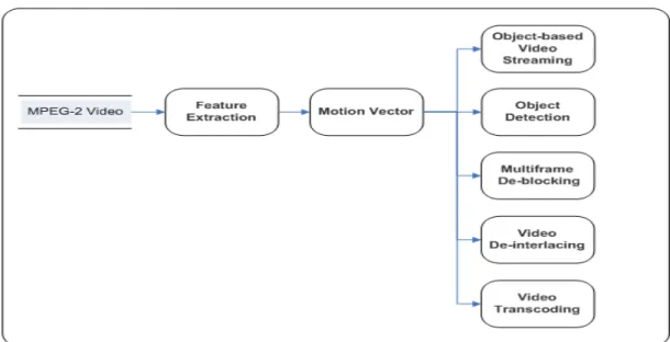
(17) and exploited in many video processing and communication applications, as depicted in Fig. 1-2. First video processing using motion vector is video object detection. Video object detection is a primary step for several video processing applications. Video object detection has two forms, either stand alone application or intermediate level form. Stand alone video object extraction applications include: 1.. Video surveillance. 2.. Vision-based control. 3.. Human-computer interfaces. 4.. Medical imaging. 5.. Robotics. Intermediate layer object extraction applications include: 1.. High level content based video retrieval.. 2.. Video event Detection.. 3.. Video Summarization and abstraction.. 4.. Video tracking.. Fig. 1-2. Video processing and communication applications using motion vectors 4.

(18) Although, much work in pixel domain [8, 9, 10, 11], deploys the visual features and motion information, very little work has been carried out in the area of compressed domain video object extraction. Motion detection in pixel domain is performed based on the motion information at each pixel location like optical flow estimation [12], which is computationally very demanding. In many cases, especially in the case of well-textured objects, the motion vector values reflect the movement of objects in the scene very well. In this thesis, object detection work has been carried out based on motion vectors to keep the processing in the compressed domain. Video streaming enables simultaneous delivery and playback of the video. This is in contrast to file download where the entire video must be delivered before playback can begin. In video streaming there is usually a short latency in the start of delivery and the beginning of playback at the client. Therefore, deploying information available in the compressed domain will make the real-time video streaming task possible and efficient. In this thesis, an efficient motion vector based approach has been investigated on video streaming. Video transcoding application is also one of the most recent topics in video processing. It touches several newly established technologies such as 3G mobile network and Mobile TV.. Mobile access to multimedia contents requires video transcoding. functionality at the edge of the mobile network for interworking with heterogeneous networks and services. Under certain conditions, the bandwidth of a coded video stream needs to be drastically reduced. Converting a previously compressed video bit stream to a lower bit rate through transcoding can provide finer and more dynamic adjustments of the bit rate of the coded 5.

(19) video bit. stream to meet various channel situations [18]–[24].. Depending on the. particular strategy adopted, the transcoder attempts to satisfy network conditions or user requirements in various ways. Since the delivery system must accommodate various transmission and load constraints, it is sometimes necessary to further convert the already compressed bitstream before transmission. This thesis addresses all the aspects of video transcoding that deals with motion vectors. In sum, motion vector features provided by video in compressed domain is an important cue for analysis and communication applications. Thus, the need becomes clear for reliable and accurate motion vector information for those approaches deploying the motion information [2,3,13-27]. However, it is sometimes hard to use motion vectors due to the noise which makes further processing of the data almost impossible. Besides, motion vectors are still far from ideal, as the key motion estimation is carried out using coarse area-correlation method that has proven inefficient in terms of accuracy. Some researchers [28] elaborate on the noise in motion vector due to the camera noise and irregular object motion. It is realized [32] that the motion fields in MPEG streams are quite prone to quantization errors, and at the encoding steps might be not correctly matched in low-textured area. However, typical samples in the motion vector field are usually inaccurate [33,34]. These defects can be combated with robust error recovery schemes that repair motion fields and eliminate the noise. Consequently, we can produce reliable motion vector features to be used in video processing and communication applications. Therefore, in this thesis, we introduce techniques that can overcome those defects and produce more reliable motion vectors. These techniques perform processing on the extracted motion vector fields from motion frames. Specific refinement techniques 6.

(20) remove noise and smooth motion vectors. It makes the resulting filtered data more representative of the original motion vectors and more reliable for use in further compressed domain video processing and communication applications.. 1.3 Organization of the thesis The rest of the thesis is organized as follows. Chapter 2 presents the background and related work. Chapter 3 analyzes the motion vectors and their limitations. Chapter 4 describes the proposed motion vector schemes. Chapter 5 presents the proposed object detection approach.. Chapter 6 describes object based video streaming technique.. Chapter 7 discusses and provides video transcoding mechanism. Chapter 8 presents the experimental results. Chapter 9 draws the conclusion and suggests the future directions.. 7.

(21) Chapter 2 Background and Related Work Since we want to make use of motion vectors and DCT coefficients, we have to understand the MPEG video compression standard. In addition, good explanation for the motion vector production should be stated.. 2.1 Background information for MPEG and motion vectors With recent improvements in processing and storage technologies, many personal computing systems have the capacity to receive, process, and render multimedia objects (e.g., audio, graphical and video content). While MPEG-1 and MPEG-2 can significantly reduce the number of bits needed to represent a video sequence without appreciable degradation of image quality, the compressed format does not lend itself to easy video processing. The MPEG coding includes information in the bit stream to provide synchronization of audio and video signals, initial and continuous management of coded data buffers to prevent overflow and underflow, random access start-up, and absolute time identification. The coding layer specifies a multiplex data format that allows multiplexing of multiple simultaneous audio and video streams as well as privately defined data streams. The basic scheme of MPEG is to predict motion from frame to frame in the temporal direction and then to use Discrete Cosine Transform (DCT) coefficients to organize the redundancy in the spatial directions. MPEG uses two inter-frame coding techniques: predictive and interpolative. This results in three basic picture types in an MPEG stream: I-, P- and B-pictures. An Ipicture is completely intra-coded. It provides access points for random access but only 8.

(22) with moderate compression. A P-picture is predictably coded with reference to a past picture, which can be either an I- or a P-picture. A P-picture will in general be used as a reference for future prediction. A B-picture is bi-directionally coded. It is similar to a Ppicture, but requires both a past and a future reference picture for prediction. B-pictures provide the highest amount of compression. The relation between the three picture types is illustrated in Fig. 2-1.. Fig. 2-1: A Group Of Pictures (GOP) structure. GOP is based on a random access requirement. Typically, a starting point is needed at least once in every 0.4 seconds. Providing an I frame every twelve frames correlates to starting with an I frame in every 0.4 seconds. To decode the bit stream, the I frame is first decoded followed by the first P frame. The two B frames in between the I frame and the P frame are then decoded. The primary purpose of the B frames is to reduce noise in the video by filling in or interpolating, between the I and the P frames, typically over a 33 or 25 millisecond picture period without contributing to the overall signal quality. 9.

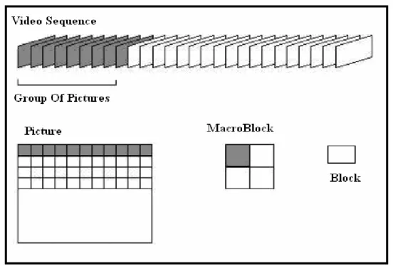
(23) The B frames and P frames contain the motion information. The I frame has no motion values and stores the DCT information of the original frame of the video sequence. An interesting aspect of the MPEG-4 standard, necessary to support such interactive features, is that a video frame is actually defined as a number of video objects, each assigned to their own video object plane (VOP). When the compressed multimedia object is accessed for use, it is decompressed in accordance with the compression scheme used to compress the multimedia object, e.g., using the Inverse Discrete Cosine Transform (IDCT). Once decompressed further analysis of the multimedia objects may then be performed. The difficult challenge in the design of the MPEG compression algorithm is the following. On one hand the quality requirements demand a very high compression ratio not achievable with intra-frame coding alone. On the other hand, the random access requirement is best satisfied with pure intra-frame coding.. Inter-frame coding can. achieve high compression while it does not promise random access. This requires a delicate balance between intra-frame and inter-frame coding. Fig. 2-2 shows the hierarchical structure of an MPEG video stream, which is represented by the following six layers: Video Sequence: A sequence is the top level of the MPEG video coding. It is composed of several groups of pictures (GoPs) used as a random context access unit. For video analysis, information, such as frame rate, picture width and height, aspect ratio, and video bit rate, can be obtained from the video sequence layer. Group of Picture (GoP): A GoP consists of a series of pictures and is used as a random access unit for video coding. Information, such as the number of pictures in the GoP, is available from the GoP layer. A picture is the primary coding unit and consists of several 10.

(24) slices. Information, such as picture type (I, P and B) and motion vector resolution, is available for video analysis from this layer. A slice is used as a re-synchronization unit and consists of several macroblocks. Macroblock: A macroblock contains a 16×16 pixel region of luminance component and the spatially corresponding 8 × 8 pixel region of each chrominance component since chrominance components are sampled at half the luminance resolution. It thus has four 8×8 luminance blocks and two 8 × 8 chrominance blocks. For video analysis, the macroblock layer provides the type of coding (intra versus non-intra) and the motion vector. Block: A block is 8×8 pixels in size and is the unit of subsequent Discrete Cosine Transform (DCT). It provides 64 DCT coefficients (either of original pixel values or of the residues after the motion compensation). MPEG uses a component color representation for each color pixel, namely one luminance (Y) and two chrominance components (Cb and Cr). The conversion, from YCbCr to conventional RGB space, can be carried out by a linear mapping (a 3×3 matrix).. Since the human visual system (HVS) is most sensitive to luminance. component, the Y values are encoded at the full resolution. The HVS is less sensitive to the chrominance information. As a result, the two chrominance components are encoded at half the resolution of their luminance counterpart. This considerably reduces the amount of information to be compressed.. 2.1.1 Motion Compensation Motion-compensated prediction assumes the current picture can be modeled as a translation of the picture at some previous time. The local unit used in MPEG is macroblock. This is the result of a trade-off between the coding gain provided by the 11.

(25) motion information and the cost associated with coding the motion information. Each macroblock in a P-picture is matched to the most similar group of 16 × 16 pixels in its reference picture. This process is called motion estimation.. Fig. 2-2 Stream structure for MPEG video. Motion estimation obtains the motion vector, which is the displacement between a macroblock and its predictor candidate, by minimizing a cost function measuring the mismatch between the two macroblocks. If no match is found within a specified search range, a macroblock will be intra-coded. A macroblock in a P-picture can also be skipped, meaning it is exactly the same as the macroblock at the same location in the reference picture. As a result, a skipped macroblock will be motion vector of zero. For each macroblock in a B-picture, it can be forward-predicted, backward predicted, or bi-directionally predicted. Consequently, its motion information consists of one forward motion vector, one backward motion vector, or both of the forward and backward motion vectors. Once the motion vector for each macroblock is estimated, the prediction error or residue, the 12.

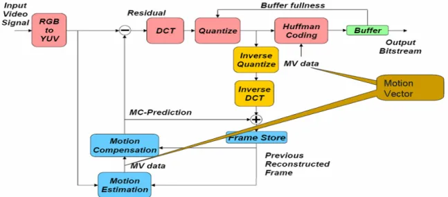
(26) difference between a macroblock and its matched candidate, is calculated. The residue will then be intra-coded by the DCT transform method.. 2.1.2 DCT Transform Both still-image and difference image (residue) signals have a very high spatial redundancy. Because of the block-based nature of the motion compensation process and a relatively straightforward implementation, the two dimensional Discrete Cosine Transform (DCT) is chosen as the basis of compression of each I-picture and of the residue images from P- and B-pictures. The Forward and Inverse DCT are defined as follows:. Among the 64 DCT coefficients, c(0, 0) is the weighted value for the DCT basis function, referred to as the DC term. The other 63 DCT coefficients, c(i, j), for i, j = 0, 1, ..7 are referred to as the AC coefficients.. From the Forward DCT, we have 64. coefficients for each block. These coefficients are quantized, zig-zag ordered, run-length and then Huffman coded to reduce spatial redundancy. Fig. 2-3 presents a typical video encoder/decoder including all the described stages for decoding and encoding. In addition, the motion vector flowing path is stated. 13.

(27) Fig. 2-3 Typical video encoder/decoder flowchart. 2.2 Related Work The need for reliable and accurate motion vector information is clear for those approaches that are employing the motion information [2,14-16,27-29,33,35,36]. However, a refining process has to be performed on the motion vectors. Some researchers applied the motion vector refinement in the pixel domain. This implies they were actually filtering the visual features. Some [1] matched the filtered visual feature with the motion vector. Others used filtered visual features as a postprocessing step [29]. Although [1,29] claimed that the motion vector refining results can be improved significantly, drawbacks remain. These drawbacks include the increment in computational complexity, as well as the other already mentioned drawbacks of doing video processing in the pixel domain. Median filter and modified median filter [33,37] has been used for refining motion vectors. However, results in [59,61] prove the usage of median filter is insufficient and unreliable for high level applications. In these approaches [33,37], the time consumption is high due to the computation complexity resulting from partially processing in the pixel 14.

(28) domain. Approach [37] used P,B frames in order to extract motion vectors. [33] applied refining for the motion vector magnitude only, while in our proposed scheme, refinement is applied on both magnitude and direction, which will result in a more accurate and reliable outcome. The approach in [38] is based on an assumption which consider motion vector refining results from median filter is the closest to true motion vector. In addition a fuzzy set membership function and some statistical approach were used to decide the motion vector robustness and filter it out accordingly. However their basic assumption is not accurate according to what has been discussed earlier regarding the weakness and the limitation of median filter in smoothing motion vectors. In addition, the proposed post processing operations after using the motion vectors smoothing operation are sophisticated and time consuming. Hence it is not suitable for real time application. Scheme in [39] performs motion vector refinement by using simple thresholding for both motion vector magnitude and direction. For general purpose, applying simple thresholding to the magnitude and the direction of the motion vector is not effective enough to remove random noisy vectors in the background region. In addition, the thresholding process based on experimental results only is not deterministic.. 15.

(29) Chapter 3 Motion Vector Analysis 3.1. Motion Information Extraction from MPEG video. The sparse motion vectors from the compressed video stream are extracted. For the computation efficiency, only the motion vectors of P-frames are used for object detection algorithm since in general, in a video with 30 fps, consecutive P-frames separated by two or three B-frames, are still similar and would not vary too much. Besides, it must be noted that B frames are just ‘interpolating’ frames that hinge on the motion information provided in P frames and therefore using them for the concatenation of displacements would be redundant. Therefore, it is sufficient to use the motion information of P frames only in several video processing applications.. 3.2. Motion Vector Noise Analysis. Due to the complexity of motion vector calculation in the encoding process, the raw motion vectors extracted from an MPEG or H.26x video stream may contain incorrect motion vectors and noise as will be proved later on in this section. Therefore, the realization of any approach which utilizes motion vector has to contain a refining mechanism to eliminate the incorrect motion vectors and noise. Fig. 3-1 state the relation between the processing-time and the information level. Traditional methods start from the bottom level to detect raw motion information from the original video. In contrast, our proposed scheme starts from the middle level by extracting the motion vectors directly from the MPEG videos. The top level operates on specified and semantically filtered motion information. This represents a significant saving in computational cost in comparison to traditional approaches. This will be proven 16.

(30) in the result and discussion section.. Fig. 3-1 Video processing level and cost effect. 3.2 Motion vector limitations Motion estimation can be seen as an optimization problem. The brute force methods simply try all possible vectors, in a predefined range, to be sure to obtain the global optimum of the criterion function. Also, there are efficient approaches that test only the most likely motion vectors. This likelihood is usually determined by spatial or temporal proximity, and, consequently temporal and spatial prediction vectors have been popular in the efficient motion estimation algorithms.. Depending on the motion estimation. algorithm used, the quality of the resulting motion vector is different. At the decoder/receiver side, it is unknown what type of motion estimation algorithm was used at the encoder/transmitter side, so one must assume, as a worst case situation, that the MPEG motion vectors are optimized for an efficient compression, and that they do not represent true motion vectors. In sum, motion vectors in compressed domain suffer form the following limitations: 1. A homogeneous background could produce strange and long inconsistent vectors when small change of light happens in a heterogeneous way. More specifically, 17.

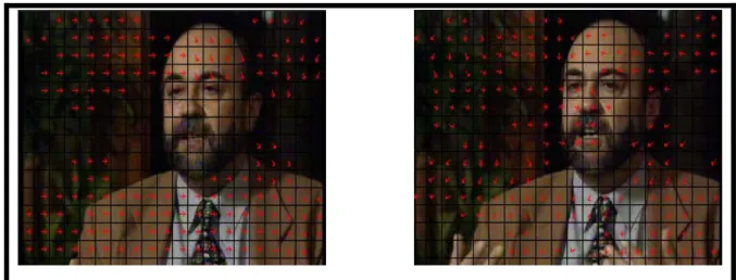
(31) periodical structures and noise in picture areas with little detail may cause such inconsistent vectors. 2. In MPEG data streams, it is uncertain that all motion vectors are transmitted within the data stream. 3. The motion vectors lack effective representation and its strong noise makes further processing almost impossible. 4. Researchers [28] elaborate on the noise in motion vector due to the camera noise and irregular object motion. However, it is known that the motion vectors in MPEG-1/2 may not represent the true motion of a Macro-block. 5. The macroblock scheme makes the usage of motion vector hard. For example, in object detection application, objects that are too small are simply ignored and object contours are distorted [29,30,31]. 6. It is realized [32] that the motion fields in MPEG streams might have incorrectly matched in low-textured area. Fig. 3-2 and Fig. 3-3 show examples of extracted motion vectors from “walking person” and “interview” video streams respectively. Some of these motion vectors are either irrelevant or false. For example, in background areas or static object there exist ‘motion vectors,’ which contradict with basic idea of motion vector.. 18.

(32) Fig. 3-2 extracted motion vectors from video stream “walking persons”. Fig. 3-3 extracted motion vectors from video stream “interview”. 3.3. Motion Vector Noise Model. These described limitations above do not exclude the motion vectors entirely from use in high quality video processing applications. When an appropriate post-processing is applied, the motion vectors can be made useful. More specifically, when the receiver is able to determine the quality of the motion vectors, and when it is able to improve the quality of the motion vectors so that they meet certain criteria for the intended processing, the motion vectors can be used. Now, we describe the motion vector noise model.. A motion vector can be. represented in Eq. (3.1). v(i,j) is the sum of the true reliable motion vector t (i, j ) and the noise n(i, j ) , where i,j are the indices of the corresponding macroblock in each frame. 19.

(33) v ( i , j ) = t (i , j ) + n (i , j ). (3.1). Noise within the content of the motion vector fields can generally be expressed as independent noise, which can often be described by an additive noise model.. 20.

(34) Chapter 4 Motion Vectors Refinement Approaches Several motion refinement approaches have been proposed and conducted. These approaches are developed in different domains, such as spatial domain, temporal domain, texture domain. Spatial domain filter concerns the motion vector refinement based on the spatial correlations among the motion vectors in each motion frame, such as P-frame.. 4.1 Gaussian Based Motion Vector Refinement Noise within the content of the motion vector fields can generally be expressed as independent noise, which can often be described by an additive noise model. Additive noise is evenly distributed over the frequency domain, whereas a reliable motion vector exists at low frequencies. Hence the noise is dominant for high frequencies and its effects can be reduced by using some kind of low pass filter. This can be done either with a frequency filter or with a spatial filter, but a spatial filter is preferable as it is computationally less expensive than a frequency filter. Fig. 4-1 states the general scheme for Gaussian based motion vectors refinement. First step extracts the motion vectors from the MPEG video stream.. Then, noise. elimination based on Gaussian filter controlled by the so called configuration box is conducted. Configuration box is the module in charge of allowing users to interact and adjust the Gaussian filter parameters to optimize the noise elimination process. In the literature there are many spatial filters such as Gaussian, median and mean filters. We use the Gaussian filter due to its desirable characteristics. The Gaussian filter has the significant characteristic of its step response containing absolutely no overshoot. The Gaussian filter uses a kernel that represents the shape of a Gaussian distribution. Fig.. 21.

(35) 4- 2 illustrates the Gaussian distribution. Gaussian functions are separable. As a result, a Gaussian convolution can be implemented by a 1D horizontal convolution followed by a 1D vertical convolution. Using this decomposition, the number of operations decreases significantly. Hence the Gaussian filter can fit real time applications.. Fig. 4-1 General scheme for Gaussian based motion vector refinement. The Gaussian function is uni-modal. The Gaussian filter provides gentler smoothing and preserves the crucial motion vector value better than mean filter. Gaussian functions are rotationally symmetric in two dimensions.. Thus, the amount of smoothing is. independent of the direction. This property implies that no bias is introduced. The degree of smoothing is parameterized by the standard deviation of the filter σ . We can maintain this value interactively to control the result of motion vector filtering. Hence, using the Gaussian filter gives some flexibility, which makes the refinement scheme possible for a wide range of applications.. 4.1.1 Smoothing of Motion Vector Field Up to this stage we have the motion vectors extracted from motion frames in MPEG. Then, we will pass the motion vector magnitude and direction values to the Gaussian filter where using two values instead of only one makes the refinement process more robust and meaningful.. First we need to configure Gaussian filter by setting the 22.

(36) parameters such as σ . Such parameters have a crucial effect in the smoothing process. Thus we implement a user interface “configuration box” as demonstrated in Fig. 4-3 where users can interactively change the parameters for filtering until the optimal filter performance is obtained.. Fig. 4-2. 2-D Gaussian distribution with mean (0,0) and σ =1. First, the value of σ is chosen to maximize the smoothing. By experiment, the value. σ =1.2 gives us the best performance for Gaussian filter. [36] explored the use of a Gaussian filter, and excellent results can be achieved with a σ value between 1.0 and 1.5. Smaller values of σ (values less than 1.0) tend to leave slightly inhomogeneous cluster patterns as shown in Fig. 4-4. While larger values tend to form regularly spaced clusters patterns as shown in Fig. 4-5. This proved to be in agreement with our experiment over the motion vector smoothing. Concerning other parameters, the kernel size was chosen to be 3X3 since the window search in our object detection is 3X3 as well. Moreover, the kernel size is recommended to be 3X3 in the interest of reducing the cost of computation. The last parameter to determine is the iteration, the number of times to repeat the convolution step. This will affect the degree of enhancement and the accuracy of the filter. Empirically we find the value 5 to be a suitable value, taking into consideration the performance and the execution time. 23.

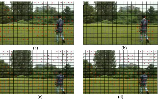
(37) Fig. 4-3. The user interface for motion vector smoothing. Fig. 4-4 The effect of using small σ value, σ =0.002. Fig. 4- 5. The effect of using large σ value, σ =3.5. Fig. 4-6(a)(b)(c)(d) show the performance of motion vector refinement using no filter, Gaussian filter, median filter and mean filter, respectively. The value of σ has been chosen to be 1.2 and kernel size to be 3X3. The presented results show clearly the advantage of using Gaussian filter comparing to the usage of mean and median filters 24.

(38) Fig. 4-7 represents the same idea for the different video clip “walking person”.. (a). (b). (c). (d). Fig. 4-6 Extracted motion vectors from “interview video” after applying (a) Without processing (b) Gaussian filter (c) Mean filter (d) Median filter.. (a). (b). (c). (d). Fig. 4-7 Extracted motion vectors from “walking person video” after applying (a) Without processing (b) Gaussian filter (c) Mean filter (d) Median filter. 25.

(39) 4.2 Cascade Filter Based Motion Refinement Through our experiment we noticed that there is a weakness in the single Gaussian filter performance when the object location is in the frame border. This can be explained due to the lack of information in the neighborhood near the border. We use a cascade filter which is composed of a Gaussian filter followed by median filter to improve the performance. Fig. 4-8 and 4-9 schematically illustrates the cascade filtering.. Fig. 4-8 Refinement scheme overview. Fig. 4-9 Cascade filter design. The deficiency in frame border will disappear due to the median filter’s characteristic of rearranging the motion vectors value to become more representative of the true motion vector and better aligned. The proposed cascade filter boosts the performance. In addition, the computational complexity is low. Both the Gaussian and median filters are available as a readily implemented component in both hardware and software. The resultant motion vectors resulting after filtering are less noisy. Execution time of deploying the refined motion vectors will be reduced significantly compared to that without using a filter. Although we are adding another block for filtering, the efficiency is almost the same or even better in terms of execution time for the entire object detection process.. 4.3 Temporal based Motion Vector Refinement 26.

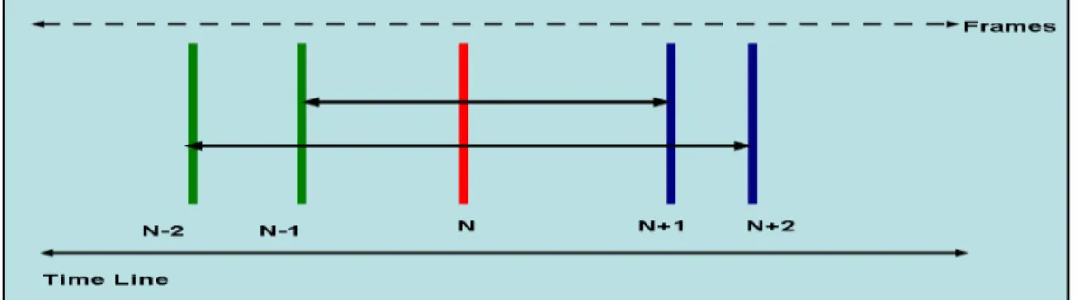
(40) Temporal filter component is designed based on the temporal adjacent neighborhood of a macroblock. The main idea is that a ‘fine’ motion vector should not have its direction altered in a drastic manner. Fig. 4-10 states the relation among the current, successive and precedent frames. Motion vectors in these frames are temporally correlated. Each frame is affected by its successive and precedent frames. The closer the frame is, the more correlated and contributing to its neighbor, so MVN+1 is twice important than MVN+2 to current motion vector MVN. Eq(4.1) states the temporal refinement.. MVnew = (2(MVN+1 + MVN-1) + (MVN+2 + MVN-2))/6 + ½(MVN). (4.1). where MVnew is the refined motion vector in temporal domain, and N-1,N-2,N,N+1,N+2 are frame numbers in the video sequence.. Fig. 4-10 Relation among the current fame and other frames in temporal domain.. 4.4 Texture Based Motion Vector Refinement Up to this stage, motion vectors have been refined temporally and spatially. Important domain is the texture domain due to the fact that well textured motion vector has good motion vector value. This will lead us to adaptively refine the motion vectors based on texture. To calculate the texture for each motion vector we analyze the AC components of the DCT coefficients, thus staying in the compressed domain. The proposed scheme was inspired by this fact. The MPEG compressed video provides one motion vector for each macroblock The 27.

(41) DCT information from I-frames are readily available in MPEG stream. Thus we need to spend too much time in decoding the MEPG stream. Hence our approach can fit the real time application environment.. 4.4.1 Texture energy computation Important regions are distinguished from background using the distinguishing texture characteristics. The video analysis is performed directly in the DCT compressed domain using the intensity variation encoded in the DCT domain. Therefore, only a very small amount of decoding is required. In some applications, researchers do use either the horizontal intensity variation or vertical intensity variation. For example, in the text detection, it is generally approved that text regions possess a special texture because text usually consists of character components which contrast the background and, at the same time, show a periodic horizontal intensity variation due to the horizontal alignment of characters. In addition, character components form text lines with approximately the same spacing [42,43]. As a result, text regions can be segmented using texture features. In this thesis we propose a texture-based motion vector filter which operates directly in the DCT domain in video. The DCT coefficients in MPEG video [45], which capture the directionality and periodicity of local image blocks, are used as measures to identify high texture regions. Therefore, we will be able to treat each motion vector accordingly. Each unit block in the compressed images is classified based on local horizontal, vertical and diagonal intensity variations. In summary, DCT coefficients in compressed domain images capture the local periodicity and directionality features in the spatial domain. We examine the coefficients of each DCT block of a frame. By noting the correlation of frequency distribution in each block and the corresponding spatial features (see Fig. 4-11(a)), we may choose to 28.

(42) process further only those blocks which meet certain criteria. For example, to detect edges, only the medium and high frequency components are needed [10], and only the blocks containing coefficients in that range are considered for decompression. In addition, we may use the feature distribution patterns of DCT coefficients to choose subregions of a representative video frame (see Fig. 4-11(b)). Blocks containing high and medium frequencies are selected, and only the set of blocks that correspond to a ‘large’ region in the spatial domain are selected. The computational savings that result from this simple step are many folds. The DCT processing need not be applied to the entire image, resulting in additional savings in time. Since a smaller image area is analyzed, all subsequent steps, such as detecting straight edges, or detecting long edges can be completed more effectively. To gain some insight into the DCT spectrum, Fig. 4-12(a) shows an input image and Fig. 4-12(b) shows the absolute values of the DCT coefficients directly extracted from the compressed domain of the intensity image. Each subimage in Fig. 4-12(b) represents one DCT block of the input image. The blocks, from top to bottom, indicate horizontal variations, with increasing frequencies; and from left to right, indicate vertical variations, with increasing frequencies. The blocks on the top row, from left to right represents zero vertical frequency and increasing horizontal frequencies. Top left blocks represent the low frequency components, contain most of the energy, while the high frequency channels, which are located at the bottom right corner of each subimage, are mostly blank. These observations indicate that the blocks spectrums capture the directionality and coarseness of the spatial image. For all the vertical edges in the input image, there is a corresponding high frequency component in the horizontal frequencies, and vice versa. 29.

(43) Furthermore, diagonal variations are captured by the energies around the diagonal line. This example illustrates that the DCT domain features do characterize the texture attributes of an image. The basis images are placed with increasing horizontal frequency from left to right, and increasing vertical frequency from top to bottom.. (a) (b) Fig. 4-11 (a) frequency distribution (b) block distribution [11]. Therefore, we can design Directional Texture Energy Map in DCT domain as shown in Fig. 4-13, by assigning a directional intensity variation indicator for each AC coefficient as the following. H: Horizontal intensity variation V: Vertical intensity variation D: Diagonal intensity variation We are processing in the DCT domain to obtain the directional intensity variation, called directional texture energy, using only the information in the compressed domain. Note that the operating units are the 8X8 blocks in I-frames.. Fig. 4-12-a: Input image. Fig. 4-12-b: The absolute values of the DCT coefficients directly extracted from the compressed domain. 30.

(44) For each DCT block, we compute the Horizontal energy Eh by summing up the absolute amplitudes of the horizontal harmonics of the block: which are marked as H in the directional texture energy map. For each DCT block, we compute the vertical energy Ev by summing up the absolute amplitudes of the vertical harmonics of the block: which are marked as V in the directional texture energy map. For each DCT block, we compute the diagonal energy Ed by summing up the absolute amplitudes of the diagonal harmonics of the block: which are marked as D in the directional texture energy map. Finally, we will calculate the average energy Ea for each block, which is the average value of the Vertical energy, Diagonal energy and Horizontal energy as in Eq.( 4.2).. ⎧12*Eh +5*Ed +12*Ev ⎪ 29 ⎪ ⎪11*Eh +7*Ed +11*Ev ⎪ 29 Ea = ⎨ ⎪11*Eh +6*Ed +12*Ev ⎪ 29 ⎪12*E +6*E +11*E h d v ⎪ 29 ⎩. (4.2). We will update Motion vector values based on the Ea as described in the following procedure.. Fig. 4-13: Directional Texture Energy Map in DCT 31.

(45) For every macrblock :. Motion _ Vector new. 100 * E a ⎧ % , Ea < Et ⎪⎪ Motion _ Vector old ∗ Et =⎨ ⎪ ⎪⎩ Motion _ Vector old , E a ≥ Et. We have used an adaptive threshold value. The following diagram in Fig. 4-14 describes the process for texture filtering in the frame level. The I-frame has no motion values and it stores DCT information of the original frame. Though I-frame provides no motion information, we still could grasp the frame texture, and propagate that information to the P frames as described in next section. Fig. 4-14 clearly states the operation in algorithmic way, where, after knowing the frame type we send this frame for its specific module. If this frame is an I-frame, then we know it contains the DC value and AC components. Thus, we can calculate the texture energy as stated before according to the previous procedure and texture energy map. After we propagate those values into P-frames then we perform the texture filter on the motion vector values. Alternative procedure for texture and edge calculation has been proposed for providing additional texture information. The details of the approach are presented herein. First of all the energy map is redefined according to Fig. 4-15. New energy detentions are introduced. Atot : Total Energy AD : Diagonal Energy AH : Horizontal Energy AV : Vertical Energy AFin : Final Energy 32.

(46) Energy calculation is based on the redefined texture energy map as show in Fig. 4-15.. To make a decision regarding the texture of each macroblock the following procedure is deployed.. Fig. 4-14: Flowchart of texture based motion vectors refinement.. 33.

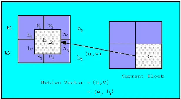
(47) Fig. 4-15 Redefined Texture Energy Map. 4.4.2 Reconstruction of DC Images To propagate the texture information into the p frames we need to reconstruct the DC images for P frames. In the following, only the reconstruction of the luminance DC images is discussed. Chrominance DC images can be similarly reconstructed. For intracoded I-pictures, reconstruction of such DC images is trivial since the DCT DC value of each block can be directly obtained from an MPEG stream. The DC values of an intra-coded macroblock in a P-picture can be similarly obtained as those in an I-picture. Extraction of exact DC values for motion compensated macroblocks in a P-picture is given in [32] and is computationally expensive. Here we describe an approximation method proposed by [112].. A motion. compensated macroblock in a P-picture has a motion vector and four blocks of DCT coded motion compensated errors.. The motion vector allows us to trace back the. macroblock to its matching counterpart in the previous reference picture. Each of the four luminance blocks will be matched in a location in the reference picture as shown in Fig. 4-16. The matching block may overlap as many as four blocks in the reference picture.. Assume that the DC values of the reference picture are available and the 34.

(48) luminance variance within each block is small.. Then the DC value of the motion. compensated block in a P-picture can be approximated by taking the overlapping area of the four blocks in the reference picture pointed by the motion vector plus its DC value of the residues as in Eq.(4.3).. Where DC(bi) is the DC value of block i in the reference picture, and wi and hi are the overlapping width and height respectively. Their values are related to the motion vector (u,v) as follows: w1=w3=u, w2=w4=8-u, h1=h1=v and h3=h4=8–v. The term DC(bresidue ) is the residue DC values of the current block. bi is block number . For those motion compensated macroblocks with both forward and backward motion vectors, their DC values can be calculated as the average of those reconstructed from the previous reference picture and the future reference picture plus the DC values of their residues. Using the above method, we can reconstruct a DC image sequence from an MPEG stream, no matter what picture types (I, P or B) it contains.. Fig. 4-16 illustrations on the relation among the current block, reference block and motion vector. 35.

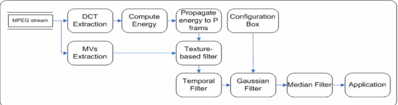
(49) 4.5 Overview of the Motion Vector Refinement System The proposed system architecture for motion vector refinement now is shown in Fig. 4-17. For an input video stream, we extract the motion vectors from inter-frames such as P-frame. In practice, P-frames only are suggested to be processed in order to reduce the computational complexity. Meanwhile, we will extract the DCT coefficients from I frames, including the DC coefficient, and the AC components as well. Then, we will pass the DCT coefficients into a module to calculate the texture of each frame. Later, we will propagate this texture information into the inter-frames using the DC image reconstruction technique described early. After that, we will filter each motion vector based on its texture value. Then, we pass the filtered motion vectors to temporal filter component. This filter is derived from the temporal adjacent neighborhood of a macroblock.. After obtaining the. motion vector field’s magnitude and direction values, we pass these values through the Gaussian filter. Meanwhile, filter parameters such as standard deviation and kernel size are initialized to obtain the optimal performance. We then pass these filtered motion vectors into a specific application. Furthermore, we use the median filter because it does not alter motion vector values. Rather, it simply rearranges motion vectors, not altering the values contained within any motion vector. Hence the median filter is used to repair potential irregularities introduced by the previous filter processing and in order to straighten up some single motion vector which has been influenced.. 4.6 Adaptive Motion Vector Refinement This section introduces for adaptive motion vector refinement technique in spatial domain. Previously, the adaptation process is supported in texture domain, but in certain 36.

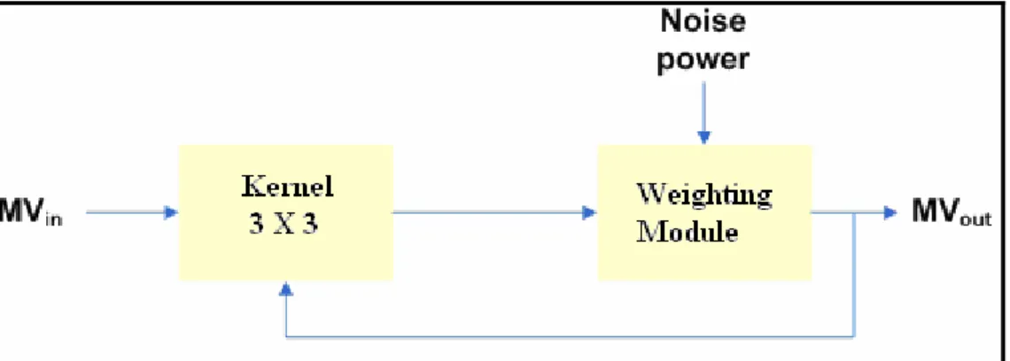
(50) cases, neither the texture domain nor the temporal domain techniques are applicable. Therefore, a spatial domain adaptive motion vector refinement is proposed.. Some. application like video transcoding puts hard limitation on the refinement techniques and resources. Thus we develop a strict and very resource limited technique which lies only in spatial domain. In [1,12,41] the analysis showed that the differential reconstruction error causes incoming motion vectors to deviate from optimal values.. Fig. 4-17. The proposed motion vector refinement system architecture. Therefore, a fine motion vector can be obtained by refining the incoming motion vectors according to the proposed scheme. Depending on the application, various types of noise can be distinguished. Gaussian additive noise is a commonly applied model to represent the noise as obtained in motion vector signals. However, impulsive noise originating from uncertain defection can be recognized and requires an individual approach in order to get optimal performance. In this chapter we will focus on the Gaussian additive noise, and optionally try to defeat the impulsive noise effects.. Fig. 4-18 The overview architecture of the proposed adaptive motion vector refinement scheme 37.

(51) In Fig. 4-18, we introduce a general view of the proposed motion vector refinement scheme. Our scheme consists of two parts; the first part is the noise level estimator. It is used to estimate the noise power for every frame processed. This parameter will be used in the noise reduction block to generate the filter parameters. The second part is the noise reduction block. It is a general spatial filter which uses the correlation between the current motion vector and its neighbourhoods. The spatial filter is shown in Fig. 4-19. It is a recursive spatial filter and includes a kernel and weighting module. The kernel as shown in Fig. 4-12 consists of a 2D window of motion vectors MV (i) (i=0, l...8) where MV(0) is the central motion vector that will be filtered. MV(1)-MV(8) are the neighbourhoods of MV(0).. Fig. 4-19. Block diagram of the noise reduction block. MV1. MV2. MV3. MV4. MV0. MV5. MV6. MV7. MV8. Fig. 4-20. Kernel of 3X3 motion vectors. In the weighting module, the output motion vector can be calculated as in Eq.(4.4).. 38.

(52) MV out =. ∑W. i∈ N 1. 1. ( i ) ∗ M V ′( i ) + ∑ W 2 ( i ) ∗ MV ( i ). ∑W. i∈ N 1. i∈ N 2. 1. (4.4). (i ) + ∑ W 2 (i ) i∈ N 2. where N1 = {1, 2, 3, 4} and N2 = {5, 6, 7, 8} are sets of neighbourhood vectors. And the weights of each motion vector are defined as:. W1 (i ) = z1 K (i ). i ∈ N1. W 2 (i ) = z 2 K (i ). i ∈ N2. (4.5) (4.6). where z1 and z2 are the parameters related to the position of the weighted Motion vector. To use more information of refined motion vector, we have z1 =3* z2. K(i) is a parameter related to the local noise power and the absolute difference between the weighted neighbourhood motion vector (MV(i)) and the current input motion vector (MV(0)). K(i) function is defined in Eq.(4.7).. K (i ) = e. ⎛ MV ( i ) − ( MV ( 0 ) + λ ) ⎞ −⎜ ⎟ Noise Power ⎝ ⎠. 2. ,. (4.7). where λ is a parameter related to the local noise power of current input motion vector. It is ranged within − Noise Power ≤ λ ≤ Noise Power . λ can be estimated by Eq.(4.8).. ⎧. ⎫. λ = arg min⎨ ∑ MV ′(i) − ( MV (0) + λ j ) + ∑ MV (i) − ( MV (0) + λ j ) ⎬ λj. ⎩i∈N1. i∈N 2. ⎭. (4.8). The weighting function K(i) indicates that the contribution of a neighborhood motion vector to the current centre motion vector is exponentially related to the difference between them. The smaller the difference, the more contribution the neighbourhood motion vector has. This property can eliminate the Gaussian noise effectively.. 4.6.1 Noise Power Estimator 39.

(53) We introduce a method for noise power estimation. This noise estimation algorithm allows refinement at varying motion vector conditions. To increase the adaptation of the concepts, a simple but effective new noise power estimation algorithm was designed that controls the parameters of the noise reduction. The Noise Power Estimator is used to estimate the noise power for every frame processed. Noise power values are used in the noise reduction. The difference of every motion vector with its previous and next motion vector is calculated and the accumulated differences are delayed for four motion vectors and further accumulated into a variable entitled AC_DIFF. The Noise Power of each frame is updated as in Eq.(4.9).. ⎧ Noise Power ( f ) − 1 NPI > Thershold t ΛNoise Power ( f ) Noise Power ( f ) = ⎨ ⎩ Noise Power ( f ) + 1 NPI ≤ Thershold t ΛNoise Powe( f ). (4.9). Noise Power (f) is the noise power of frame f and the Thresholdt is an experimentally optimized constant defined as: Thresholdt = ( Number of Motion Vector * 60) / 100. (4.10). The number of Motion vector is defined as the total number of motion vectors in each frame. The Noise Power Indicator (NPI) is defined NPI =. ∑. (4.11). B(MV). MV. where B(MV) is a binary variable assigned to every motion vector. ⎧ 1, Noise Power ( f ) < AC _ DIFF ( MV ) < 1 . 5 Noise Power ( f ) B ( MV ) = ⎨ else ⎩0,. (4.12). and AC_DIFF is the local noise power estimator calculated as a sum of Absolute Differences AC _ DIFF ( MV ) =. 4. ∑. F ( MV + n ) + F ( MV + n − 1). n =1. 40. (4.13).

(54) Chapter 5 Object Detection in Video Streams 5.1 Introduction Over the last decade, there has been growing interest in content representation of video sequences with rapid developments in multimedia and internet applications. New representation of video sequences needs to be constructed not only in compact forms, but also as semantic entities for content-based functionalities such as retrieval and manipulation. Video semantic object is a perfect content representation. To bridge the semantic gap and achieve a high level of content based representation, some previous works [46] select video object plane supported by the MPEG-4 standard as the underlying video patterns for video content representation and feature extraction. However, the major problem is that semantic video object extraction in general does not perform automatically. A good performance still needs human's interaction at the current stage. Recently, many researches on human visual system show that moving objects can be easily distinguished and have more attraction of visual attention. Approaches [47,48] extract moving objects as semantic objects for content representation. Moving objects can provide a good pattern for motion-related high-level semantic analysis. Studies on visual attention and eye movements [49,50] have shown that humans generally can only attend to a few areas in an image. Even with unlimited viewing time, attention will continue to focus on these few areas rather than scan the whole image. An increasing number of researchers are now exploring the intermediate-level processing, shifting the focus of attention away from pixel-based indicators to high-level processing. 41.

(55) In [51], authors use motion information to construct salient map for video sequence. Salient region extraction based on saliency map [31] provides a good starting point for semantic-sensitive content representation. However, perceived salient region extraction for image or video is still an unsolved problem. One reason is that video sequence has more context information than single image. Hence, low-level features are often not enough to classify some regions unambiguously without the incorporation of high-level and human perceptual information into the classification process. Another reason for the problems is perception subjectivity. Different people can differ in their perception of high-level concepts. Thus a closely related problem is that the uncertainty or ambiguity of classification in some regions cannot be resolved completely. A basic difference between perceptions and measurements is that, in general, measurements are crisp whereas perceptions are fuzzy [52]. Moreover moving object detection is a useful tool for intelligent video browsing/analysis and video surveillance systems.. In order to meet the real-time requirement, no computationally intensive. operation is included. Video object detection is a key operation for content-based video coding multimedia content description, and intelligent signal processing. New functionalities like object manipulation and scene composition can be achieved because the video bitstream contains the object shape information. However, the shape information of moving objects may not be available from the input video sequences; therefore, segmentation is an essential task. In addition, many multimedia communication applications have real-time requirement, and an efficient algorithm for automatic video segmentation is very desirable. Motion estimation has been proposed [54] to solve this problem. If both ends of a motion vector are inside the frame difference mask, then the corresponding area is 42.

(56) part of the object. Otherwise, that area is assumed to be background. This approach has several drawbacks.. First, the motion estimation is not very. accurate near the object boundary where highest accuracy is required. Second, motion estimation can deal with the translation type of motion only. If other forms of movement are involved, motion vectors may fail to track the object motion. Also, motion estimation is a computationally intensive operation and this process will dramatically increase the complexity of the segmentation system. Motion-based video object detection has been explored, with approaches generally based on the analysis of optical flows. Compressed videos require the decompression of the sequences and the computation of optical flows, two steps computationally heavy. In this chapter we propose some methods for motion-based video object detection by motion features (mainly related to motion vector) and by motion-based spatial segmentation of frames, in a fully automatic way. Our idea is to use motion vectors as an alternative to optical flows. It does not require a decompression of the stream and saves us from computing optical flows. Additional computational economy comes from having one motion vector each macroblock. This makes the algorithms faster than those that work with dense optical flows. Experimental results reported at the end of this chapter show that MPEG motion compensation vectors are suitable for this kind of applications.. 5.2 Related Work and Background Moving object detection techniques have been studied extensively [53-56] for purposes such as video content analysis as well as remote surveillance. For example, in [53] optical flow method is employed in pixel domain and a moving object is detected. 43.

(57) when similar optical flow is found in a certain area. In [54], a moving object is detected using inter-frame difference after compensating camera work. As for the compressed data domain processing, the [55] proposes the detection method by finding objects with similar motion vectors in a picture after compensating global motion. However, from experimental point of view, flat background was often falsely detected as a moving object since random motion vectors appear in the flat background [56]. Previously the authors have proposed a method to detect moving object area on MPEG coded data domain [56] by analyzing the motion vectors and DCT coefficients. In P- and B- pictures, moving objects are detected by analyzing motion vectors and spatial-temporal correlation of motion. In addition, by analyzing coding characteristics of intra macroblocks (MBs) in P- and B-pictures and by investigating temporal motion continuity in I-pictures, moving objects in these situations have been also detected in intra MBs.. 5.3 Object Detection and Extraction We started by thresholding motion vectors before the detection process in order to achieve more robust performance.. Motion vectors with magnitude equal to or. approaching zero are recognized as undesirable and hence are not taken into consideration. On the contrary, motion vectors with larger magnitude are considered more reliable and are therefore selected.. 5.3.1 Object Detection Algorithm An object detection algorithm is used to detect potential objects in video shots. Initially, undesired motion vectors are eliminated. Subsequently, motion vectors that have similar magnitude and direction are clustered together and this group of associated 44.

(58) macroblocks of similar motion vectors is regarded as a potential object. Details are presented in the object detection algorithm. Fig. 5-1 shows the graphical user interface for the moving object detection module, as video clips can be traced and monitored while this module detects each object in real time.. Fig. 5-1 Graphical user interface for object detection. The Object Detection Algorithm Input: P-frames of a video clip Output: object sets {Obj1 , Obj2 , … ObjN } where N is the total number of regions in Pframe and ObjN means the Nth object of the P-frame. Each object size is measured in terms of number of macroblocks. 1. Cluster motion vectors that are of similar magnitude and direction into the same group with region growing approach. 1.1. Set search windows (W) size 3×3 macroblocks.. 1.2 Search all macroblocks (MB) within W, and compute the difference ( diffMag k and diffAng k ) of motion vector (MV) magnitude ( MV ) and direction ( ∠MV ) between center MVcenter and its neighboring eight motion vectors MVk within W. 45.

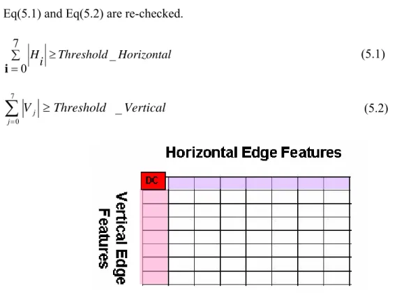
(59) 1.2.1. diffMag = abs( | MVcenter | - | MVk | ). 1.2.2. diffMag = abs( ∠MVcenter - ∠MVk| ). 1.2.3 EDGEk = detect_edge(MBk). ,. where k ∈ [1,8] and MVcenter is the MV in the center position of W MVk ∈ MVs within W except MVcenter 1.2.4. For all 1≦ k ≦ 8, flag. ⎧1, diffMag k < TMag and diffAng k < T Ang and EDGEk Fk = ⎨ otherwise ⎩0, where TMag is the predefined threshold for MV magnitude and TAng is the threshold for MV direction 1.2.5. 8. If ∑. k =1. Fk ≥ 6. , mark Fcenter of MVcenter as 1, where Fcenter is the flag of the. center MV within W. Otherwise, set all flags within W to 0. 1.3. Go to step 1.2 until all macroblocks are processed.. 1.4. Group macroblocks that are marked as 1 into the same cluster.. 1.5. Compute each object center and record its associated macroblocks.. 5.3.2 Edge Detection using AC coefficients We use the predefined two edge features [28] to derive edges. The two horizontal and vertical edge features can be formed by two dimensional DCT of a block. In the DCT domain, the edge pattern of a block can be characterized with only one edge component, which is represented by projecting components in the vertical and horizontal directions, respectively. The edge features from the DCT basis images is. 46.

(60) shown in Fig. 5-2. In order to extract the edge features the following conditions in Eq(5.1) and Eq(5.2) are re-checked. 7 ∑ H ≥ Threshold _ Horizontal i i=0 7. ∑V j =0. j. (5.1). ≥ Threshold _ Vertical. (5.2). Fig. 5-2 Horizontal and vertical edge feature in DCT domain. If the test results for the Eq.(5.1) and Eq.(5.2) conditions are ‘true’ and ‘false’, respectively, it is defined that the block contains a vertical edge. For a horizontal edge in the block, the converse is true, i.e. the tests have to be ‘false’ and ‘true’, respectively. If both tests are ‘true’, the block contains a diagonal edge and it is further tested to determine its orientation using the polarities of the first coefficients: H1 and V1. That is, the coefficients have the same polarities (V1 & H1 = positive, or V1 & H1 = negative) for a 45-degree diagonal edge, and different polarities (V1 = positive and H1 = negative, or V1 = negative and H1 = positive) for a 135-degree diagonal edge. Therefore, we are now able to detect the edge block in each frame to decide is edge block or not.. 5.4 Object detection overview After all, we can introduce the whole object detection system including the motion vector refinement and our proposed video object detection. Then we use the proposed 47.