SIMULATION OF HYDRAULIC SHOCK WAVES BY HYBRID FLUX-SPLITTING SCHEMES IN FINITE VOLUME METHOD
J.-S. Lai * G.-F. Lin ** W.-D. Guo ***
Hydrotech Research Institute Department of Civil Engineering
National Taiwan University National Taiwan University
Taipei, Taiwan 10617, R.O.C. Taipei, Taiwan 10617, R.O.C.
ABSTRACT
In the framework of the finite volume method, a robust and easily implemented hybrid flux-splitting finite-volume (HFF) scheme is proposed for simulating hydraulic shock waves in shallow water flows. The hybrid flux-splitting algorithm without Jacobian matrix operation is established by applying the advection upstream splitting method to estimate the cell-interface fluxes. The scheme is extended to be second-order accurate in space and time using the predictor-corrector approach with monotonic upstream scheme for conservation laws. The proposed HFF scheme and its second-order extension are verified through simulations of the 1D idealized dam-break problem, the 2D oblique hydraulic shock-wave problem, and the 2D dam-break experiments with channel contraction as well as wet/dry beds. Comparisons of the HFF and several well-known first-order upwind schemes are made to evaluate numerical performances. It is demonstrated that the HFF scheme captures the discontinuities accurately and produces no entropy-violating solutions. The HFF scheme and its second-order extension are proven to achieve the numerical benefits combining the efficiency of flux-vector splitting scheme and the accuracy of flux-difference splitting scheme for the simulation of hydraulic shock waves.
Keywords : Hybrid flux-splitting finite-volume scheme, Shallow water flows, Flux-vector splitting,
Flux-difference splitting.
1. INTRODUCTION
Mathematically, the system of two-dimensional (2D) shallow water equations is a time-dependent set of non-linear partial differential equations of hyperbolic type. The most challenging feature of this hyperbolic system is that it may contain the discontinuous solutions such as hydraulic shock waves. Numerical simulations of hydraulic shock waves are difficult due to special considerations for achieving conservative property, dealing discontinuity and capturing the shock wave. To capture discontinuities without spurious oscillation and produce less numerical dissipation, several high- resolution total variation diminishing (TVD) schemes for the hyperbolic conservation laws have been proposed in the literature [1,2]. Most of them adopt a first-order upwind scheme as a basis to achieve higher- order accuracy. Many first-order upwind schemes have been developed in the literature [1~5]. They can be generally categorized into two classes: the flux- difference splitting (FDS) scheme and the flux-vector splitting (FVS) scheme [2]. The FDS-type schemes use an approximate solution of the local Riemann problem, such as the Osher scheme [5], the Roe scheme [3], the Harten, Lax and van Leer (HLL) scheme [2], etc.
The FVS-type schemes split the flux vector into positive and negative parts, such as the van Leer splitting (VLS) scheme [1,2], the Steger-Warming splitting (SWS) scheme [4], the local Lax-Friedrichs splitting (LLFS) scheme [6], etc.
Based on the FDS-type or FVS-type schemes, the high-resolution TVD schemes have been introduced into hydraulics and employed to solve shallow water flows. For instance, Mingham and Causon [7] and Hu et al. [8] used the HLL scheme as a basis to develop the second-order TVD schemes. Tseng [9] and Tseng and Chu [10] adopted the popular Roe scheme to develop the high-resolution schemes. Their schemes resulted in good numerical resolutions of the shock waves. However, the Roe scheme needs matrix calculation and requires the entropy fix to avoid entropy-violating solutions. Lin et al. [11] adopted reliable first-order FVS-type schemes as bases to establish finite-volume component-wise TVD schemes. Erduran et al. [12] evaluated the performances of five typical upwind schemes, including the Osher, HLL, HLLC, Roe and SWS schemes. They found that the Osher scheme is the most accurate without any entropy fix. In addition, the SWS scheme is the most efficient but it produces an unphysical glitch for problems involving rarefaction shock.
Recently, an attempt in the development of upwind schemes for solving the hyperbolic conservation laws is to construct the so-called hybrid flux-splitting schemes that make use of the concepts from both FDS and FVS. Liou and Steffen [13] proposed an advection upstream splitting method (AUSM) to solve the Euler equations in gas dynamics. Lately, several researchers improved the AUSM and developed the so-called AUSM-type schemes [14~18]. These hybrid flux-splitting schemes can be interpreted as the hybridizations between the FDS and FVS. They are more accurate than the FVS-type schemes and more efficient than the FDS-type schemes. Besides, they are rather simple to implement because they do not require the Jacobian matrix operations. Hence, applying the hybrid flux-splitting algorithm seems attractive to solve hydraulic shock waves in shallow water flow problems.
The purpose of this study is to propose a hybrid flux-splitting finite-volume scheme for simulating shallow water flows. Adopting the finite volume method (FVM), the 2D shallow water problem is dealt with as a series of local one-dimensional (1D) Riemann problems in the direction normal to the cell interface. A hybrid flux-splitting algorithm based on the AUSM is established by solving the Riemann problem to obtain the cell-interface numerical fluxes. According to the algorithm, the first-order hybrid flux-splitting finite- volume scheme, namely the HFF scheme, is then proposed. Its second-order extension is achieved based on the monotonic upstream schemes for conservation laws (MUSCL) method. The proposed HFF scheme and its second-order extension are applied to simulate hydraulic shock waves in shallow water flows, including the 1D idealized dam-break problem, the oblique hydraulic shock wave problem and the dam-break experiments with channel contraction as well as wet/dry beds. Meanwhile, the HFF-based schemes are compared with several well-known and commonly-used schemes to evaluate their numerical performances.
2. SHALLOW WATER EQUATIONS
In the conservative form, the 2D shallow water equations (SWE) can be written as
Q F G S t x y ∂ + ∂ + ∂ = ∂ ∂ ∂ (1) in which 2 2 Q ; F ; 2 hu h gh hu hu hv huv ⎡ ⎤ ⎡ ⎤ ⎢ ⎥ ⎢ ⎥ ⎢ ⎥ =⎢ ⎥ =⎢ + ⎥ ⎢ ⎥ ⎢ ⎥ ⎣ ⎦ ⎣ ⎦ 0 2 0 2 0 G ; S ( ) ( ) 2 x fx y fy hv huv gh s s gh s s gh hv ⎡ ⎤ ⎢ ⎥ ⎡ ⎤ ⎢ ⎥ ⎢ ⎥ =⎢ ⎥ =⎢ − ⎥ ⎢ ⎥ ⎢ − ⎥ ⎣ ⎦ ⎢ + ⎥ ⎢ ⎥ ⎣ ⎦ (2)
where Q is the vector of conserved variables; F and G
are the flux vectors in the x- and y-directions, respectively; h is the water depth; u and v are the depth-averaged velocity components in the x- and y-directions, respectively; g is the acceleration due to gravity; S is a source term; Sfx and Sfy are the bed
friction slopes in the x- and y-directions, respectively; and S0x and S0y are the bed slopes in the x- and
y-directions, respectively.
3. NUMERICAL FORMULATIONS 3.1 Numerical Discretization by Finite Volume
Method
A cell-centered finite volume method (FVM) is employed to discretize Eq. (1) numerically. Integrating Eq. (1) over the control volume Ω and using the divergence theorem yields the basic equation of FVM: dW dl dW t Ω ∂Ω Ω ∂ + ⋅ = ∂
∫∫
Q∫
E n∫∫
S (3)in which n is the outward unit vector normal to the boundary ∂Ω; dW and dl are the area and arc elements, respectively; and the integrand E ⋅n is the normal flux vector in which E= [F, G]T.
The vector of conserved variables Q is assumed constant within arbitrary control volume. Thus, the basic vector equation of the FVM can be obtained by discretizing Eq. (3) as M m m n m 1 d A L A dt = +
∑
= Q E S (4)where A is the area of a cell, m is the index for the side of the cell, M is the total number of sides of a cell , m
n
E
is the normal flux across each side m separating two neighboring cells, and Lm is the length of the side.
Applying the rotational invariance of the governing Eq. [19], one can obtain the intercell flux normal to each side m as 1 1 ( ) cos sin ( ) [ ( ) ] ( ) ( ) n = θ + θ = θ − θ = θ− E Q F G T F T Q T F Q (5) where θ is the angle between the outward unit vector n
and x-axis; Q T Q= θ( ) =[ , , ]q q q1 2 3 T =[ ,h hu hvn, t]T is
the vector transformed from Q; ( ) [ , 2/ 2 n hu gh = + F Q 2, ]T n n t
hu hu v is the transformed normal flux; un and vt
are respectively the flow velocity components in
x (normal) and y (tangential) directions, which are un=ucosθ+vsinθ and vt=vcosθ−usinθ; and T(θ)and
T(θ)−1 are the transformation and inverse transformation
1
1 0 0 1 0 0
( ) 0 cos sin , ( ) 0 cosθ sin 0 sin cos 0 sin cos
− ⎡ ⎤ ⎡ ⎤ ⎢ ⎥ ⎢ ⎥ θ =⎢ θ θ⎥ θ =⎢ − θ⎥ ⎢ − θ θ⎥ ⎢ θ θ⎥ ⎣ ⎦ ⎣ ⎦ T T (6) Based on Eq. (5), Eq. (4) can be rewritten as
1 1 ( ) ( ) M m m d A dt − L A = +
∑
θ = Q T F Q S (7)The conserved quantity can have different values in each cell of the computational domain. Thus, the values of the conserved quantity are discontinuous across the interface between cells. According to the interface discontinuity, the estimation of the interface fluxF Q( )in Eq. (7) can be simplified into a problem
for solving a series of local 1D Riemann problems in the direction normal to the cell interface.
3.2 Estimation of Cell Interface Flux F Q( )
The local 1D Riemann problem, an initial-value problem, in the direction normal to the cell interface is written as [11,19] [ ( )] 0 t x ∂ + ∂ = ∂ ∂ Q F Q (8a) with 0 ( , 0) 0 L R x x x ⎧ < = ⎨ > ⎩ Q Q Q (8b)
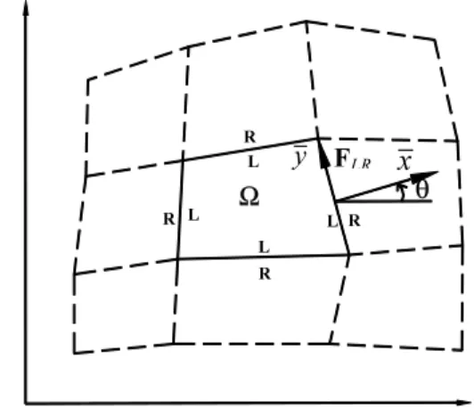
As illustrated in Fig. 1, the x axis with its origin
located at the midpoint of interface of two cells is directed to outward normal. The F Q( ) is a normal
outward flux at the origin of a local axis x. The
quantities, QL and QR , are the left and right
transformed quantities at the center of the cell interface, respectively.
The system of Eq. (8) is a time-dependent set of non-linear partial differential equations of hyperbolic type. Therefore, many FDS and FVS schemes applied to solve the Euler equations in gas dynamics may be adopted for the estimation of the cell interface flux
( )
F Q . In this paper, a hybrid flux-splitting algorithm is proposed for solving the local 1D Riemann problem in SWE. Besides, the numerical flux functions of some well-known first-order FDS-type and FVS-type schemes are reviewed herein, which are very useful for comparing with the proposed algorithm to evaluate the numerical performances. The first-order numerical flux function is denoted by F Q QLR( ,L R), which is through the cell interface between the left cell with subscript L and the right cell with subscript R.
L R L R L R R L
Fig. 1 The finite volume cell Ω and the Riemann interface
3.3 Review of FDS-Type Schemes
The FDS-type schemes are derived based on the approximate solutions of Riemann problem in Eq. (8). Hence, they are known as the approximate Riemann solvers. Here we present the numerical flux functions of three FDS schemes, including the Osher, the Roe and the HLL schemes.
The Osher scheme is obtained using the Riemann invariant to determine the flux through the cell interface [5]. The numerical flux function of the Osher scheme is 3 Osher 1 1 1 ( , ) [ ( ) ( )] 2 2 k k LR L R L R k k d Γ = = + −
∑∫
λ F Q Q F Q F Q R Q (9) where Γk is the integration path with three subcurves,λk(k= 1, 2, 3) are the eigenvalues and R(k) (k= 1, 2, 3)
are the eigenvectors. They are expressed as
1 un c, 2 un, 3 un c λ = − λ = λ = + (10) (1) (2) (3) 1 0 1 , 0 , 1 n n t t u c u c v v ⎡ ⎤ ⎡ ⎤ ⎡ ⎤ ⎢ ⎥ ⎢ ⎥ ⎢ ⎥ =⎢ − ⎥ =⎢ ⎥ =⎢ + ⎥ ⎢ ⎥ ⎢ ⎥ ⎢ ⎥ ⎣ ⎦ ⎣ ⎦ ⎣ ⎦ R R R (11)
where c= gh is the local wave celerity. In Eq. (9),
the approximation of the integration path is needed. More details about the Osher scheme can be found in [1,2].
The Roe scheme is constructed based on the linearized form of Eq. (8). Roe’s numerical flux function [3] is 3 Roe 1 1 1 ( , ) [ ( ) ( )] 2 2 k LR L R L R k k k = = + −
∑
α λ F Q Q F Q F Q R (12)where λk, αk and Rk are respectively the average
approximate eigenvalues, wave strengths, and eigenvectors. They can be expressed as follows:
Ω θ
FLR x
1 un c, 2 un, 3 un c λ = − λ = λ = + (13) 1 12 h hc un , 2 h vt, 3 21 h hc un ⎡ ⎤ ⎡ ⎤ α = ⎢∆ − ∆ ⎥ α = ∆ α = ⎢∆ + ∆ ⎥ ⎣ ⎦ ⎣ ⎦ (14) (1) (2) (3) 1 0 1 , 0 , 1 n n t t u c u c v v ⎡ ⎤ ⎡ ⎤ ⎡ ⎤ ⎢ ⎥ ⎢ ⎥ ⎢ ⎥ =⎢ − ⎥ =⎢ ⎥ =⎢ + ⎥ ⎢ ⎥ ⎢ ⎥ ⎢ ⎥ ⎣ ⎦ ⎣ ⎦ ⎣ ⎦ R R R (15) with , , R L n nR nL t tR tL h h h u u u v v v ∆ = − ∆ = − ∆ = − (16)
in which h, c , un, and vt are called the Roe
average values. They can be obtained from
2 2 1 , ( ) 2 L R L R h= h h c= c +c (17) , nL L nR R tL L tR R n t L R L R u h u h v h v h u v h h h h + + = = + + (18)
The HLL scheme assumes the estimates SR and SL as
the smallest and largest signal velocities in the solution of the Riemann problem [20]. Applying the integral form of the conservation laws in appropriate control volumes, one can have the HLL numerical flux function as HLL ( ) if 0 ( , ) ( , ) if 0 ( ) if 0 L L * LR L R L R L R R R s s s s ⎧ ≥ ⎪ =⎨ < < ⎪ ≤ ⎩ F Q F Q Q F Q Q F Q (19) where ( , )* L R
F Q Q represents the HLL numerical flux,
given by ( ) ( ) ( ) ( , ) R L L R R L R L L R R L s s s s s s ∗ = − + − − F Q F Q Q Q F Q Q (20)
To provide appropriate the wave speeds estimates for SR
and SL, there are several possible choices available.
Toro [20] recommend min( , ), max( , ) L nL L n R nR R n s = u −c u∗−c∗ s = u +c u∗+c∗ (21) in which 1( ) , 1( ) 1( ) 2 2 4 n nL nR L R L R nL nR u∗= u +u + −c c c∗= c +c + u −u (22)
3.4 Review of FVS-Type Schemes
The FVS technique described here was originally proposed by Steger and Warming [4] for the solution of
the Euler equations. The normal outward flux vector
( )
F Q can be decomposed into positive and negative
parts as
( )= +( )+ −( )
F Q F Q F Q (23)
where F Q+( ) and F Q−( ) are the positive and negative
split fluxes, respectively. The corresponding first- order numerical flux function is defined as
( , ) ( ) ( )
LR L R = + L + − R
F Q Q F Q F Q (24)
Then, using different forms of the split flux vector ( )
±
F Q leads to different numerical flux functions.
Here we briefly describe the numeral flux functions of three FVS-type schemes, including the VLS, SWS, and LLFS schemes.
The VLS scheme is devised based on the flow conditions [1,2]. For subcritical flow, |Fr| ≤ 1, the split
flux vector of the VLS scheme is defined as
VLS( ) ( n 2 ) / 2 t f f u c f v ± ± ± ± ⎡ ⎤ ⎢ ⎥ =⎢ ± ⎥ ⎢ ⎥ ⎣ ⎦ F Q (25) where f± = ± hc (F
r± 1)2/4 and Fr =un/c is the Froude
number. For supercritical flow (Fr > 1), FVLS+ ( )Q =
( )
F Q and FVLS− ( ) 0;Q = whereas if Fr < −1, VLS+ ( ) 0=
F Q and FVLS− ( )Q =F Q( ). Substitution of Eq.
(25) into Eq. (24) gives van Leer’s numerical flux function as VLS VLS VLS ( ) if 1 ( , ) ( ) ( ) if 1 ( ) if 1 L r LR L R L R r R r F F F + − ⎧ > ⎪ =⎨ + ≤ ⎪ < − ⎩ F Q F Q Q F Q F Q F Q (26) The SWS scheme is devised based on the eigenvalues decompositions [4]. The split flux vector is defined as
2 1 3 SWS 2 1 3 2 1 3 2 ( ) 2 ( ) ( ) 4 n(2 n ) n t h u u c u c v ± ± ± ± ± ± ± ± ± ± ⎡ λ + λ + λ ⎤ ⎢ ⎥ = ⎢ λ + λ − + λ + ⎥ ⎢ λ + λ + λ ⎥ ⎣ ⎦ F Q (27)
where λk+= max(λk,0) and λk− = min(λk,0) are the
positive and negative split eigenvalues. Substitution of Eq. (27) into Eq. (24) obtains the Steger-Warming numerical flux function as
SWS
SWS SWS
( , ) ( ) ( )
LR L R = + L + − R
F Q Q F Q F Q (28)
For the LLFS scheme [6], the estimation of the numerical fluxes simply depends on the maximum (absolute value) wave speed locally. The split flux vector can be expressed as
LLFS± ( )=12[ ( )±smax ]
F Q F Q Q (29)
where smax = max [|unL| +cL, |unR| + cR] is the maximum
wave speed. Substitution of Eq. (29) into Eq. (24) obtains the local Lax-Friedrichs numerical flux function as LLFS LLFS LLFS ( , ) ( ) ( ) LR L R = + L + − R F Q Q F Q F Q (30)
3.5 Hybrid Flux-Splitting Algorithm
According to the numerical treatment similar to the approach developed by Liou and Steffen [13], the normal outward flux F Q( ) can be decomposed into a
convective component FC and a pressure component P
as 2 2 2 0 ( ) 2 0 n n n n C n t n t hu hu gh hu hu p hu v hu v ⎡ ⎤ ⎡ ⎤ ⎡ ⎤ ⎢ ⎥ ⎢ ⎥ ⎢ ⎥ ⎢ ⎥ =⎢ + ⎥=⎢ ⎥ ⎢ ⎥+ = + ⎢ ⎥ ⎢ ⎥ ⎢ ⎥ ⎣ ⎦ ⎣ ⎦ ⎣ ⎦ F Q F P (31)
where p = gh2/2 is the hydrostatic pressure. The convective flux FC is further expressed in terms of the
mass flux (q2 =hun =hF cr ) and the vector Φ as [14] 2 1 ( ) C r n t q hF c u v ⎡ ⎤ ⎢ ⎥ = = ⎢ ⎥ ⎢ ⎥ ⎣ ⎦ F Φ (32)
Accordingly, the numerical flux FLR through the cell
interface between the left and the right cells is taken as [14] ( )c ( )p LR= LR + LR F F F (33) where ( )c LR F and ( )p LR
F are the numerical convective
flux and the numerical pressure flux, respectively. Based on the AUSM [13], the ( )c
LR F and ( )p LR F can be expressed as ( ) 2 / / 1 ( ) ( ) c LR LR L R r LR n t L R q hF c u v ⎡ ⎤ ⎢ ⎥ = = ⎢ ⎥ ⎢ ⎥ ⎣ ⎦ F Φ (34) and ( ) 0 0 p LR pLR ⎡ ⎤ ⎢ ⎥ = ⎢ ⎥ ⎢ ⎥ ⎣ ⎦ F (35)
where subscript L/R is defined as
2 if ( ) 0 / otherwise LR L q L R R ≥ ⎧ =⎨ ⎩ (36)
where ( )q2 LR is regarded as the cell-interface mass
flux, which can provide the information of wave propagation as well as value appropriate for upwinding; and pLR is the pressure flux.
To achieve the efficiency of FVS, the cell-interface mass and pressure fluxes are estimated using flux- vector-splitting formulation [4] and are expressed as
2 ( )q LR=c hLR[ Lℱ+(Fr L)+hRℱ−(Fr R)] (37) and LR p = +( ) r L L F p + −( ) r R R F p (38) with , nL nR r L r R LR LR u u F F c c ⎛ ⎞ ⎛ ⎞ =⎜ ⎟ =⎜ ⎟ ⎝ ⎠ ⎝ ⎠ (39)
where cLR= max (cL, cR) is defined as a common speed
of wave at the interface.
Various ways of defining the split Froude numbers
ℱ± and split pressures ± may be found. Liou and Steffen [13] used the van Leer splitting formulation. Wada and Liou [15] modified the van Leer splitting formulation by introducing a suitable parameter. Herein, we select the algorithm proposed by Wada and Liou [15] to split the parameters of Froude number and pressure in SWE. Based on the second-order polynomial of Froude number, ℱ± and ± are defined
as ℱ+ 2 1( 1) (1 ) (1 ) if 1 4 2 ( ) 1 ( ) otherwise 2 r r r r r r r F F F F F F F ± ± ⎧±α ± + −α ± ≤ ⎪⎪ =⎨ ⎪ ± ⎪⎩ (40) and ± 2 1 ( 1) (2 ) if 1 4 ( ) 1 ( ) otherwise 2 r r r r r r r F F F F F F F ⎧ ± ≤ ⎪⎪ =⎨ ⎪ ± ⎪⎩ ∓ (41) where 2 /(2 2 2) L L R c c c + α = + and 2 /(2 2 2) R L R c c c − α = + .
Obviously, the splitting functions in Eqs. (40) and (41) depend on the flow conditions (i.e. subcritical or
supercritical flows).
The first-order numerical flux function constructed through the algorithm in this section can be written as
HFF 2 1 ( , ) ( ) (Φ Φ ) 2 LR L R = q LR L+ R F Q Q ( ) 2 1 ( ) (Φ Φ ) 2 p LR R L LR q − − +F (42)
where |( )q2 LR| is the absolute value of ( )q2 LR. The
first term on the right hand side (RHS) of Eq. (43) is clearly not a simple average of left and right states, but rather a weighted-average mass flux. The second term on the RHS represents the numerical dissipation term, in which the dissipation coefficient |( )q2 LR| is merely a
scalar. Contrasting with the well-known Roe scheme, the proposed algorithm does not require the calculation of the Jacobian matrix.
3.6 First-Order Hybrid Flux-Splitting Finite-Volume (HFF) Scheme
Based onthehybrid flux-splittingalgorithm,the first- order scheme in the framework of FVM is constructed in this section. Euler’s method is employed for the time integration. Hence, in the HFF scheme the vector of conserved variables for the advanced step at time (n+ 1)∆t with the first-order accuracy both in space and time
is written as 1 1 (1) , , HFF , , 1 , ( ) ( ) ( ) M n n m n i j i j i j i j m i j t L t A + − = ⎡ ⎤ ∆ = − ⎢ θ ⎥ + ∆ ⎣
∑
⎦ Q Q T F Q S Q (43) where n is the time index; ∆t is the time increment; iand j are the space index in the x-and y-direction,
respectively; Ai,j is the area for the cell (i, j); Qi jn, is
the vector of conserved variables for the cell (i, j) at
time index n; and (1) HFF( )
F Q is the first-order numerical
flux, which is estimated using Eq. (42). Accordingly, the first-order numerical flux through the cell interface (i+ 1/2, j) is expressed as (1) HFF HFF HFF( )= LR ( ,L R)= LR ( ni, j, i , jn+1 ) F Q F Q Q F Q Q (44) where n i, j
Q is the vector of transformed variables for
the cell (i, j) at time index n. The computational cells
in the x-y coordinate system are illustrated in Fig. 2.
This proposed first-order hybrid flux-splitting finite- volume scheme is referred to as the HFF scheme herein. In Eqs. (43) and (44), using different numerical flux functions reviewed in Sections 3.3 and 3.4 leads to different first-order upwind schemes.
3.7 Second-Order Extension with MUSCL Approach
To achieve second-order accuracy in space and time, the predictor-corrector MUSCL approach given by Hirsch [1] is employed herein. Based on this predictor-corrector procedure, Eq. (7) is rewritten as
1 (1) , , HFF , , 1 , ˆ ( ) ( ) ( ) 2 2 M n m n i j i j i j i j m i j t L t A − = ⎡ ⎤ ∆ ∆ = − ⎢ θ ⎥ + ⎣
∑
⎦ Q Q T F Q S Q (45) O (i-1,j+1 ) O (i-1,j ) O (i-1,j-1 ) O (i,j+1 ) O (i,j ) O (i,j-1 ) O (i+1,j+1 ) O (i+1,j ) O (i+1,j-1 ) i-1/2 i+1/2 j+1/2 j-1/2 x yFig. 2 The computational cells in the x-y coordinates
and 1 1 (2) , , HFF , , 1 , ˆ ( ) ( ) ( ) M n n m i j i j i j i j m i j t L t A + − = ⎡ ⎤ ∆ = − ⎢ θ ⎥ + ∆ ⎣
∑
⎦ Q Q T F Q S Q (46) where Qˆi j, is the vector of predicted variables on thecell center (i, j); and (2) HFF( )
F Q is the second-order
numerical flux, which is estimated by solving the local Riemann problem based on data resulted from the predictor step. In the MUSCL method, the data reconstruction is needed to achieve second-order accuracy in space. The piecewise linear left and right variables, QiL+1/ 2,j and QRi+1/ 2,j, at the cell interface
(i+1/2, j) for a local Riemann problem are reconstructed
using the predicted variables and expressed as
1/ 2, 1/ 2, , , 1/ 2, 1/ 2, ˆ ( ) iL j L i j i j L R i j i j i j d d d + + + + = θ + ∆ + Q T Q (47a) 1/ 2, 1/ 2, 1, 1, 1/ 2, 1/ 2, ˆ ( ) iR j R i j i j L R i j i j i j d d d + + + + + + = θ − ∆ + Q T Q (47b) where dL
i + 1/2, j is the normal distance between the cell
(i, j) and the cell interface (i + 1/2, j), diR+ 1/2, j is the
normal distance between the cell (i + 1, j) and the cell
interface (i + 1/2, j), and ∆ = ∆ ∆i j, i j, ( i+1/ 2,j,∆i−1/ 2,j) is a
limiter function for the cell (i, j). Many limiter
functions satisfying the TVD constraint have been reported in the literature [1]. In this paper, four limiter functions are commonly used and presented as follows: (a) Superbee: ∆ =i j, sgn(∆i+1 2,j) max[0,min(2⋅ ∆i−1 2,j,∆i+1 2,j), min(∆i−1 2,j, 2∆i+1 2,j)] (48) (b) van Leer: 1 2, 1 2, , 1 2, 1 2, 1 2, 1 2, [sgn( ) sgn( )] i j i j i j i j i j i j i j + − + − + − ∆ ⋅ ∆ ∆ = ∆ + ∆ ∆ + ∆ (49) L R
(c) van Albada: 1 2, 1 2, 1 2, 1 2, , 2 2 1 2, 1 2, ( ) i j i j i j i j i j i j i j + − + − + − ∆ ∆ ∆ + ∆ ∆ = ∆ + ∆ (50) (d) Minmod: ∆ =i j, sgn(∆i+1 2,j) max[0, min(⋅ ∆i−1 2,j,∆i+1 2,j)] (51) where ∆i−1/ 2,j =Qni, j−Qi , jn−1 , ∆i+1/ 2,j=Qni , j+1 −Qi, jn , and
sgn refers to the sign-function [1]. Thus, the second- order numerical flux through the cell interface (i+ 1/2, j)
is estimated using the proposed flux-splitting algorithm with data reconstruction values and is expressed as
(2) HFF
HFF( )= LR ( iL+1/ 2,j, iR+1/ 2,j)
F Q F Q Q . The second-order
extension of the HFF scheme is denoted as the HFF-MUSCL scheme herein. The second-order scheme proposed herein is valid for the structured non-uniform grids.
3.8 Stability and Boundary Conditions
To ensure numerical stability of the proposed schemes, the time step ∆t must be restricted by the
Courant-Friedrichs-Lewy (CFL) stability condition [11], which is expressed as max ( ) CFL t 1 d ∆ ∆ = ≤ ∆ ∆ F Q Q (52)
where ∆d is the distance between the centers of two
adjacent cells.
The boundary conditions used herein are divided into two different types: the land boundary and the open boundary. For the land boundary, the velocity normal to the land is set to zero. At the open boundary, one needs the velocity or depth condition that can be obtained using the Riemann invariants [11].
4. NUMERICAL RESULTS AND DISCUSSIONS
Several typical cases tested in the literature are simulated to demonstrate the performances of the proposed schemes. These test cases include: the 1D idealized dam-break flow, the oblique hydraulic shock wave, and dam-break experiments with wet/dry bed conditions conducted by Bellos et al. [21].
Computations for these test cases were performed on a Pentium equipped with a 256 megabyⅣ te RAM.
4.1 Idealized Dam Break
The proposed schemes, namely the HFF scheme and the HFF-MUSCL scheme, are first applied to the 1D idealized dam-break problem with the exact solution. The idealized dam-break flood wave propagation in a rectangular, frictionless, and horizontal channel is illustrated in Fig. 3. A channel with 2000m in length and 10m in width is considered. The dam is located at
1000m downstream of the channel inlet. After the dam is broken instantaneously at time t = 0+, a shock
wave traveling downstream and a rarefaction wave traveling upstream are created. The initial upstream water depth hu is 10m, and downstream water depths hd
are 5, 0.1, and 0.001m, respectively. Thus, three water depth ratios hd/hu of 0.5, 0.01, and 0.0001 are
considered for numerical tests. The CFL number is set to be 0.9, and 100 computational cells (grid spacing ∆x = 20m) are used. The simulation time is 50s after the dam break. The exact solutions can be found in the literature [22].
4.1.1 Comparison of First-Order Schemes
In order to evaluate the numerical performances of the proposed first-order HFF scheme, some well-known first-order FDS-type and FVS-type schemes are used herein. The FDS-type schemes include the Osher scheme [5], the Roe scheme [3] and the HLL scheme [20], and the FVS-type schemes consist of the VLS scheme [11], the SWS scheme [4] and the LLFS scheme [11]. The numerical flux functions of these schemes are reviewed in Sections 3.3 and 3.4, and employed to estimate the first-order numerical flux in Eq. (43).
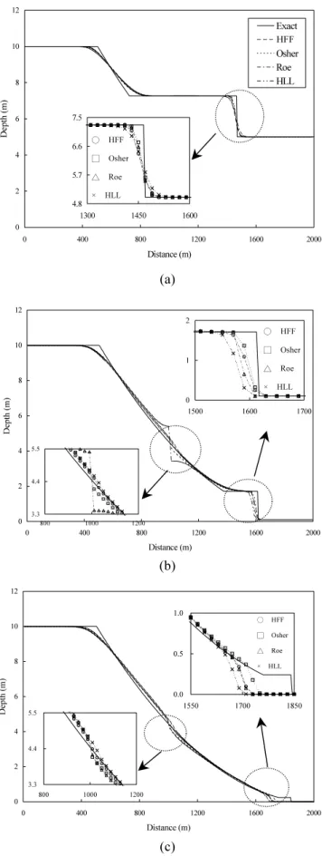
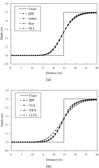
First of all, comparisons of the exact solutions with the simulated water depths using the proposed HFF scheme and the three FDS-type schemes for water depth ratios of 0.5, 0.01, and 0.0001 are made and plotted in Figs. 4(a) to 4(c), respectively. As shown in Fig. 4(a) with the close-up of the shock wave, all schemes can predict the shock wave and the rarefaction wave without any spurious oscillation produced. The HFF, Osher and Roe schemes present similar resolutions of the shock wave front, and they are more accurate than the HLL scheme. For a water depth ratio hd/hu of 0.01,
Fig. 4(b) shows that the HFF scheme produces the best resolution around the dam-site. Besides, the resolution of shock wave front using the HFF scheme is better than those using the Roe and the HLL schemes. In addition, in Fig. 4(b) with the close-up at the dam site, the Roe scheme apparently presents entropy-violating solution (rarefaction shock), whereas the HFF, Osher and HLL schemes do not.
To ensure the entropy-satisfying
Fig. 3 Aschematic representation of 1D dam-break problem
Dam
Water depth ratio=hd / hu
hu
0 1 2 1500 1600 1700 0 2 4 6 8 10 12 0 400 800 1200 1600 2000 Distance (m) De pth (m ) 0.0 0.5 1.0 1550 1700 1850 0 2 4 6 8 10 12 0 400 800 1200 1600 2000 Distance (m) De pth (m ) (a) (b) (c)
Fig. 4 Comparisons of exact solutions with simulated depths using the HFF scheme and three FDS- type schemes for water depth ratios hd / hu of (a)
0.5, (b) 0.01, and (c) 0.0001
solution, the formula of entropy correction given by Harten and Hyman [23] is employed hereafter. For a water depth ratio hd/hu of 0.0001, Fig. 4(c) shows that
applying the entropy correction to the Roe scheme obviously improves the glitch of the solution. From the simulated results presented in Fig. 4, it is found that the HFF scheme presents the best resolution in the rarefaction wave at the dam site, and it also produces better resolutions of shock wave front than those by the Roe and the HLL schemes.
Moreover, comparisons of the exact solutions with the simulated water depths using the proposed HFF scheme and the three FVS-type schemes for the water depth ratios of 0.5, 0.01, and 0.0001 are made and plotted in Figs. 5(a) to 5(b) and 5(c), respectively. The simulated results show that the HFF scheme produces the best resolution at the shock front as well as the dam site, whereas the LLFS yields the most dissipative results especially for small water depth ratio conditions.
Table 1 summarizes the relative error in L2 norm and
CPU time for different water depth ratios of 0.5, 0.01, and 0.0001 to evaluate overall numerical accuracy quantitatively. The L2 norm of water depth is defined
as [24] sim exact 2 , , 2 exact 2 , ( ) ( ) i j i j i j Y Y L Y − =
∑
∑
(53) Where sim , i j Y and exact ,i jY are respectively the simulated
and the exact solutions at cell (i, j). Comparing the
overall numerical accuracy, between the HFF and three FDS-type schemes, the Osher scheme yields the smallest L2 norm of water depth, whereas the HLL gives
the largest one. The overall numerical accuracy of the HFF scheme is better than those of the Roe and HLL schemes. Moreover, in the three test cases of the different water depth ratios, the HFF scheme consumes averagely 39%, 81%, and 19% less CPU time than the Osher scheme, the Roe scheme and the HLL scheme, respectively. For the comparisons of the HFF and three FVS-type schemes, the HFF scheme presents the best numerical accuracy, whereas the LLFS scheme gives the most diffusive one. The CPU time consumed by the HFF scheme is almost the same as that by three FVS-type schemes. Thus, it is concluded that the HFF scheme does combine the accuracy of the FDS scheme and the efficiency of the FVS scheme.
4.1.2 Comparison of Limiters
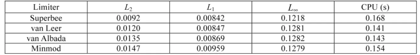
The influences of the limiters on the numerical solutions are further investigated herein. The HFF- MUSCL scheme coupled with four limiter functions, namely the Superbee, van Leer, van Albada and Minmod limiters, are considered in the test case of the water depth ratio of 0.01. To evaluate numerical accuracy and efficiency quantitatively, Table 2 summarizes the CPU time and the error norms of L2, L1,
and L∞. The L1 and L∞ norms are defined as [24]
○ HFF □ Osher △ Roe × HLL 3.3 4.4 5.5 800 1000 1200 3.3 4.4 5.5 800 1000 1200 0 1 2 1500 1600 1700 ○ HFF □ Osher △ Roe × HLL 0 2 4 6 8 10 12 0 400 800 1200 1600 2000 Distance (m) De pth (m ) Exact HFS Osher Roe HLL 4.8 5.7 6.6 7.5 1300 1450 1600 ○ HFF □ Osher △ Roe × HLL HFF
Table 1 The L2 norms and the CPU time for the idealized dam-break problem using seven first-order upwind
schemes
hd / hu= 0.5 hd / hu= 0.01 hd / hu = 0.0001
Class Scheme L2 CPU (s) L2 CPU (s) L2 CPU (s)
Hybrid HFF 0.0176 0.064 0.0364 0.079 0.0207 0.098 FDS Osher 0.0160 0.091 0.0328 0.109 0.0185 0.135 Roe 0.0178 0.118 0.0368 0.142 0.0221 0.175 HLL 0.0220 0.078 0.0424 0.094 0.0261 0.115 FVS VLS 0.0198 0.063 0.0392 0.076 0.0244 0.093 SWS 0.0213 0.066 0.0413 0.079 0.0264 0.098 LLFS 0.0245 0.062 0.0579 0.075 0.0383 0.092 (a) (b) (c)
Fig. 5 Comparisons of exact solutions with simulated depths using the HFF scheme and three FVS-type schemes for water depth ratios hd / hu
of (a) 0.5, (b) 0.01, and (c) 0.0001
sim exact sim exact
, , , , 1 exact exact , , max max i j i j i j i j i j i j Y Y Y Y L L Y ∞ Y − − =
∑
=∑
, (54)Table 2 shows that the Superbee limiter has the best numerical accuracy but costs the most computational time. The van Leer limiter costs the least CPU time, and it has the smaller error norms than those of the van Albada and Minmod limiters. The van Leer limiter is used throughout this paper.
4.1.3 Comparison of Second-Order Schemes
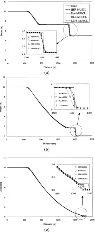
To demonstrate the numerical performance of the proposed second-order HFF-MUSCL scheme, it is compared with the commonly-used second-order TVD schemes, including the Roe-MUSCL [25,26], HLL- MUSCL [7,8] and LLFS-MUSCL [6]. These three TVD schemes are second-order extensions from the Roe, HLL and LLFS schemes, respectively. All second- rder schemes selected herein are based on the MUSCL method and adopt the van Leer limiter function in Eq. (49) to avoid the spurious oscillations. Comparisons of the above four second-order TVD schemes for water depth ratios of 0.5, 0.01, and 0.0001 are shown in Figs. 6(a) to 6(c), respectively. Compared with the simulated results presented in Section 4.1.1, it is obviously found that the simulated results for shock and rarefaction waves by the second-order schemes are better than those by the first-order schemes. In the test case of a water depth ratio of 0.5, four schemes present almost identical resolutions at the shock front. For the extreme cases with water depth ratios of 0.01 and 0.0001, as respectively shown in Figs. 6(b) and 6(c), the HFF-MUSCL scheme presents the best resolution at the shock front, whereas the LLFS-MUSCL yields the most diffusive one. To evaluate the overall numerical accuracy among these four second-order TVD schemes, Table 2 summarizes the L2 norm and CPU time. As
listed in Table 3, apparently the HFF-MUSCL scheme gives the smallest L2 norm, whereas the LLFS-MUSCL
scheme presents the largest one. Furthermore, the HFF-MUSCL and LLFS-MUSCL schemes consume about the same CPU time, and they are more efficient than the Roe-MUSCL and HLL-MUSCL schemes. Consequently, the HFF-MUSCL scheme has the inherent properties of numerical performance from the
Table 2 The L2, L1, L∞ norms and the CPU time for the idealized dam-break problem using the second-order
HFF-MUSCL scheme with four limiters, in the test case of the water depth ratio hd / hu of 0.01
Limiter L2 L1 L∞ CPU (s)
Superbee 0.0092 0.00842 0.1218 0.168
van Leer 0.0120 0.00847 0.1281 0.141
van Albada 0.0135 0.00869 0.1282 0.143
Minmod 0.0147 0.00959 0.1279 0.154
Table 3 The L2 norms and the CPU time for the idealized dam-break problem using four second-order TVD
schemes
hd / hu = 0.5 hd / hu = 0.01 hd / hu = 0.0001
Scheme L2 CPU (s) L2 CPU (s) L2 CPU (s)
HFF-MUSCL 0.0091 0.138 0.0120 0.168 0.0078 0.206 Roe-MUSCL 0.0093 0.248 0.0122 0.312 0.0082 0.385 HLL-MUSCL 0.0138 0.201 0.0145 0.240 0.0112 0.297 LLFS-MUSCL 0.0155 0.134 0.0169 0.161 0.0189 0.200
Table 4 The L1 norms and the order of accuracy p for the idealized dam-break problem using the proposed HFF and
HFF-MUSCL schemes, in the test case of the water depth ratio hd / hu of 0.01
HFF HFF-MUSCL
Number
of cells Grid spacing L1 p L1 p
50 40 0.0325 − 0.00941 − 100 20 0.0195 0.77 0.00362 1.38 200 10 0.0112 0.79 0.00121 1.58 400 5 0.0064 0.81 0.00041 1.56 800 2.5 0.0037 0.79 0.00014 1.55 1600 1.25 0.0021 0.82 0.00005 1.48
first-order HFF scheme, and it essentially obtains the combining benefits: the efficiency of FVS and the accuracy of FDS. Therefore, it is very important to use an accurate, efficient and simple-implemented first- order scheme as a basis for higher-order extension. 4.1.4 Grid Convergence Study
To further investigate the influence of the grid spacing on the numerical performance, a grid convergence study known as the grid refinement study is performed herein in the test case of the water depth ratio of 0.01 with CFL = 0.8. Table 4 lists the grid information, the L1 norms and the order of accuracy p
computed from the HFF and HFF-MUSCL schemes, where the order of accuracy p is obtained by [24]
1 1 log( ) log( ) log( ) log( ) fine coarse fine coarse L L p x x − = ∆ − ∆ (55)
Where L1fine and L1coarse are the L1 norms computed
from the fine and coarse grids, respectively; ∆xfine and
∆xcoarse are the grid spacing of the fine and coarse grids,
respectively. Figure 7 shows the convergence curves for the HFF and HFF-MUSCL schemes with varying grid spacing, where the grid spacing is normalized by the finest grid spacing (i.e. ∆x = 1.25m). Comparing with the first-order HFF scheme, results obviously show the significantly improved accuracy of the HFF-MUSCL scheme using the same grid spacing.
Besides, as shown in Table 4, the order of accuracy computed from the HFF scheme is averagely about 0.8 for all of the tested grid spacing. It is lower than the theoretical order of accuracy (i.e.p= 1). The average order of accuracy for the HFF-MUSCL scheme is about 1.5, which is also lower than the theoretical value (i.e.p = 2). The discrepancy between the computed and theoretical p is most likely due to the non-linearity in
the solution, the presence of shock wave, the TVD constraints and perhaps other factors [24]. Nevertheless, the results verify that the proposed HFF and HFF-MUSCL schemes properly converge to the exact solution as the grid size is refined. An almost grid independent solution is achieved using the HFF-MUSCL scheme with the finest grid spacing, as shown in Fig. 7.
4.2 Oblique Hydraulic Shock Wave
An oblique hydraulic shock wave (also called the oblique hydraulic jump) problem is simulated to test the 2D shock-capturing ability of the proposed schemes. As shown in Fig. 8, an oblique hydraulic shock wave is generated when a converging vertical boundary is deflected through an angle δ inward the steady supercritical channel flow. The oblique hydraulic shock wave originating at point Ο is formed with an angle of β by producing an abrupt increase in water
(a)
(b)
(c)
Fig. 6 Comparisons of exact solutions with simulated depths using the HFF-MUSCL and three commonly-used second-order TVD schemes for water depth ratios hd / hu of (a) 0.5, (b) 0.01, and
(c) 0.0001
depth. The simulation conditions used herein are the same as those in the literature [8~11]. The angle between the converging wall and the flow direction is set to be δ = 8.95°. The initial conditions corresponding to a Froude number of 2.74 are given as: the water depth of 1m, the velocity component u of
8.57m/s and v of zero. At the upstream inflow
boundary, thesupercritical inflow boundary conditions
0.000 0.005 0.010 0.015 0.020 0.025 0.030 0.035 0 4 8 12 16 20 24 28 32 36
Normalized grid spacing
L 1 no rm HFF HFF-MUSCL
Fig. 7 Convergence curves using the first-order HFF scheme and the second-order HFF-MUSCL scheme for the water depth ratio hd / hu of 0.01
x (m) y( m) 0 10 20 30 40 0 5 10 15 20 25 30 E G H Shock Front O
Fig. 8 The geometry and the computational mesh for the 2D oblique hydraulic shock wave problem of h= 1m, u= 8.57m/s and v= 0m/s are given. At the downstream outflow boundary, the transmissive boundary conditions are imposed [20]. The computational mesh with 40 × 30 nonrectangular cells is illustrated in the Fig. 8. The computational time step is 0.04s. In order to obtain a steady-state solution, a convergence criterion is defined in terms of the relative error R: 1 2 , , 5 2 , ( ) 1.0 10 ( ) n n i j i j n i j h h R h + − − =
∑
≤ ×∑
(56)where hi jn, and hi jn,+1 are the local water depths at the
time steps n and n+ 1, respectively.
In this section, the HFF scheme is compared with the aforementioned six first-order schemes. For comparisons of the HFF and three FDS-type schemes, Fig. 9(a) presents the exact solutions and the simulated results of the water depths along Line EGH illustrated in Fig. 8. The resolution of the hydraulic shock wave by the HFF scheme is better than those by three FDS-type schemes.
In a like manner, Fig. 9(b) shows the
Upstream Inflow Boundary
Table 5 Simulated results for the oblique hydraulic shock wave problem using seven first-order upwind schemes
Class Scheme L2 norm
of depth of velocity L2 norm shock angle L2 norm of CPU time for convergence criterion (s) Number of iteration
Hybrid HFF 0.049 0.0081 0.026 3.68 221 FDS Osher 0.052 0.0083 0.033 4.41 221 Roe 0.052 0.0084 0.034 7.31 220 HLL 0.054 0.0085 0.035 5.40 220 FVS VLS 0.053 0.0086 0.035 3.56 221 SWS 0.054 0.0086 0.036 3.57 225 LLFS 0.060 0.0098 0.052 3.53 267
Table 6 Simulated results for the oblique hydraulic shock wave problem using four second-order TVD schemes
Scheme L2 norm
of depth of velocity L2 norm shock angle L2 norm of CPU time for convergence criterion (s) Number of iteration
HFF-MUSCL 0.034 0.0073 0.0039 48.27 207
Roe-MUSCL 0.035 0.0073 0.0056 93.64 209
HLL-MUSCL 0.036 0.0074 0.0069 72.23 207
LLFS-MUSCL 0.045 0.0085 0.0092 49.26 221
comparisons between the HFF and three FVS-type schemes. Again, the HFF scheme yields the best resolution at the shock front, whereas the LLFS scheme obtains much dissipative solution. Table 5 lists the simulated results compared with the exact solutions, including the L2 norms of water depth, velocity, and
shock angle. The number of iteration and the CPU time for reaching the convergence criterion are also presented in Table 5. The exact solutions can be found in the literature [27]. In Table 5, it shows that the HFF scheme performs the best numerical accuracy among all first-order schemes and achieves the efficiency of the FVS-type schemes for the test case of 2D oblique hydraulic shock wave.
Three commonly-used second-order TVD schemes mentioned in Section 4.1.3 are also employed herein to compare with the proposed HFF-MUSCL scheme. All second-order schemes adopt the van Leer limiter function expressed in Eq. (49) to satisfy the TVD constraint. Figure 10 shows the exact solutions and the simulated results of the water depth profiles along Line EGH. The simulated hydraulic shock waves by the second-order schemes are sharper than those by the first-order schemes. Among them, the HFF-MUSCL scheme presents the best resolution, whereas the LLFS-MUSCL gives the most diffusive result at the shock front. Table 6 lists the L2 norm and CPU time
for convergence from the simulated results. Among all second- s than the HFF scheme. Figure 12 shows the convergence histories for the proposed HFF and HFF- MUorder schemes, the HFF-MUSCL scheme presents
the best overall numerical accuracy. It also consumes the least CPU time for convergence, which indicates the efficiency of the HFF-MUSCL scheme.
According to the HFF and HFF-MUSCL schemes, Fig. 11 shows the simulated water depth contours of the steady state solutions. Obviously, the HFF-MUSCL scheme produces better solutions than the HFF scheme. Figure 12 shows the convergence histories for the proposed HFF and HFF-MUSCL schemes. The result indicates that the second-order scheme converge faster than the first-order scheme, even with the shock. Based on the convergence criterion listed in Tables 5 and 6, the CPU time required is 3.68s for the HFF scheme, while the HFF-MUSCL scheme requires about 13 times as much. From the simulated results discussed above, the HFF scheme produces the best accuracyamong all first-order schemes. The second- order extension of the HFF scheme, i.e. the HFF-
MUSCL scheme, also performs the best numerical accuracy as well as efficiency among all second-order schemes for the test case of the 2D oblique hydraulic shock wave.
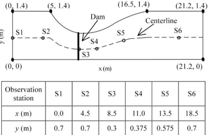
4.3 Dam-Break Experiments by Bellos et al. [21]
To demonstrate the ability of the proposed HFF scheme and its second-order extension (the HFF- MUSCL scheme) in a real dam-break scenario, the data of the dam-break experiments conducted by Bellos et al.
[21] are adopted. The channel with vertical walls is 21.2m in length and 1.4m in width at both ends. The channel has the narrowest section in the middle reach withawidth of0.6mthere. The gateislocatedatthe
(a)
(b)
Fig. 9 Comparisons of the exact solutions with the simulated depth profiles along Line EGH in Fig. 8 using (a) the HFF and three FDS-type schemes, and (b) the HFF and three FVS-type schemes
Fig. 10 Comparisons of the exact solutions with the simulated depth profiles along Line EGH in Fig. 8 using the HFF-MUSCL and three commonly-used second-order TVD schemes
(a)
(b)
Fig. 11 The contour plots of the 2D oblique hydraulic shock wave using (a) the HFF scheme, and (b) the HFF-MUSCL scheme
0.00001 0.00010 0.00100 0.01000 0.10000 0 50 100 150 200 250 Iteration number R el at iv e er ro r, R HFF HFF-MUSCL
Fig. 12 The convergence histories for first-order HFF and second-order HFF-MUSCL schemes
0.9 1.0 1.1 1.2 1.3 1.4 1.5 1.6 0 5 10 15 20 25 30 35 40 Distance (m) D ep th (m ) Exact HFS Osher Roe HLL 0.9 1.0 1.1 1.2 1.3 1.4 1.5 1.6 0 5 10 15 20 25 30 35 40 Distance (m) D ep th (m ) Exact HFS VLS SWS LLFS 0.9 1.0 1.1 1.2 1.3 1.4 1.5 1.6 0 5 10 15 20 25 30 35 40 Distance (m) D ep th (m ) Exact HFS-MUSCL Roe-MUSCL HLL-MUSCL LLFS-MUSCL 5 10 15 20 25 30 35
x (m)
5 10 15 20 25y (
m)
Contour interval = 0.05m 5 10 15 20 25 30 35x (m)
5 10 15 20 25y (
m)
Contour interval = 0.05mnarrowest section of the channel contraction, i.e. 8.5m
from the upstream end, and it can be removed instantaneously. The geometry of the experimental channel is shown in Fig. 13. The experimental series consist of setting different upstream depths and slopes of channel. Two cases of experiments are considered herein. One is a wet-bed case: upstream depth of 0.3m and downstream depth of 0.101m with a horizontal bed. The other is a dry-bed case: upstream depth of 0.15m and downstream depth of 0 m with a bed slope of 0.004. Given the same value as that analyzed by Bellos et al.
[21], the Manning coefficient is set to be 0.012 for both cases. Along the centerline of the channel from the upstream end, the data were taken at six observation stations as illustrated in Fig. 13. The total simulation time is 65s after dam break. The walls of the channel and the upstream end are land boundaries. For the wet-bed case, the measured water-depth hydrograph at
x = 18.5m is employed to provide specified depth boundary conditions at the downstream end. For the dry-bed case, a transmissive boundary condition is imposed at the downstream end.
The comparisons of the simulated water depths with the experimental data at different observation stations in the wet-bed case are made in Fig. 14. According to the wet-bed condition, the water-depth hydrographs reveal shock waves propagating and reflecting on the channel boundaries with consequent superimposition. The agreement between the simulated results and experimental data is good for the arrival of the shock wave, reflected shock and rarefaction wave. As shown in Fig. 14, both HFF and HFF-MUSCL schemes present satisfactory solutions. Nevertheless, the HFF-MUSCL scheme can obtain more accurate water-depth hydrograph that matches measured data better. Additionally, the HFF-MUSCL scheme resolves shock reflection more sharply than the HFF scheme, especially in the existence of significant depth gradient. Comparisons between experimental data and simulated water depths for the dry-bed case are shown in Fig. 15. In the dry-bed condition, an almost negligible water depth of 0.00001m is assumed at the downstream channel bed to avoid mathematical singularity [20]. In this case, the reflected shock is not created, andonlythe
x (m) y ( m) Observation station S1 S2 S3 S4 S5 S6 x (m) 0.0 4.5 8.5 11.0 13.5 18.5 y (m) 0.7 0.7 0.3 0.375 0.575 0.7
Fig. 13 The layout of the dam-break experiments of Bellos et al. [21]
(a)
(b)
(c)
(d)
Fig. 14 Comparisons of the measured and simulated water depths at Stations (a) S1, (b) S2, (c) S3, and (d) S5 in the experiment with wet-bed condition (0, 1.4) S1 (0, 0) (5, 1.4) S2 Dam S3 S4 S5 S6 (16.5, 1.4) Centerline (21.2, 1.4) (21.2, 0) 0.00 0.05 0.10 0.15 0.20 0.25 0.30 0 10 20 30 40 50 60 70 Time (s) De pth (m ) Measured HFS HFS-MUSCL 0.00 0.05 0.10 0.15 0.20 0.25 0.30 0 10 20 30 40 50 60 70 Time (s) De pth (m ) Measured HFS HFS-MUSCL 0.00 0.05 0.10 0.15 0.20 0.25 0.30 0 10 20 30 40 50 60 70 Time (s) De pth (m ) Measured HFS HFS-MUSCL 0.00 0.05 0.10 0.15 0.20 0.25 0.30 0 10 20 30 40 50 60 70 Time (s) De pth (m ) Measured HFS HFS-MUSCL
(a)
(b)
(c)
(d)
Fig. 15 Comparisons of the measured and simulated water depths at Stations (a) S1, (b) S2, (c) S4, and (d) S6 in the experiment with dry-bed condition
(a)
(b)
Fig. 16 The simulated water level profiles using the HFF and the HFF-MUSCL schemes for (a) the wet-bed case, and (b) the dry-bed case
shock wave and rarefaction wave are generated. For all observation stations, the simulated water surface profiles including the arrival time and the height of shock wave, and the overall trend agree well with the experimental results. However, the HFF scheme gives relatively more diffusive results than the HFF-MUSCL scheme.
Furthermore, Fig. 16 shows the simulated water level profiles along the centerline of the channel for both cases. It illustrates that the shock waves propagate downstream and the rarefaction waves travel upstream. The plot also shows that the HFF-MUSCL scheme presents less numerical diffusion than the HFF scheme, especially in the wet-bed case. The applications to dam-break experiments demonstrate the capability of the proposed scheme for dealing with channel friction, slope and wet/dry bed conditions.
5. CONCLUSIONS
A robust and easily-implemented hybrid flux- splitting finite-volume (HFF) scheme is proposed for modeling hydraulic shock waves in shallow water flows. The predictor-corrector MUSCL approach is employed
0.00 0.05 0.10 0.15 0.20 0.25 0.30 0 5 10 15 20 Distance (m) W ate r l ev el (m ) HFS, t = 3 sec HFS-MUSCL, t = 3 sec HFS, t = 5 sec HFS-MUSCL, t = 5 sec 0.00 0.04 0.08 0.12 0.16 0.20 0 5 10 15 20 Distance (m) W ate r l ev el (m ) Bed HFS, t = 2 sec HFS-MUSCL, t = 2 sec HFS, t = 8 sec HFS-MUSCL, t = 8 sec 0.00 0.03 0.06 0.09 0.12 0.15 0 10 20 30 40 50 60 70 Time (s) De pth (m ) Measured HFS HFS-MUSCL 0.00 0.03 0.06 0.09 0.12 0.15 0 10 20 30 40 50 60 70 Time (s) De pth (m ) Measured HFS HFS-MUSCL 0.00 0.03 0.06 0.09 0.12 0.15 0 10 20 30 40 50 60 70 Time (s) De pth (m ) Measured HFS HFS-MUSCL 0.00 0.03 0.06 0.09 0.12 0.15 0 10 20 30 40 50 60 70 Time (s) De pth (m ) Measured HFS HFS-MUSCL
to achieve the second-order-accurate extension of the HFF scheme both in space and time. The proposed HFF scheme and its second-order extension, namely the HFF-MUSCL scheme, are verified by the comparisons of exact solutions and simulated results in the 1D idealized dam-break and 2D steady oblique hydraulic shock wave problems. From the simulated results of the 1D idealized dam-break problem, it is found that the HFF scheme presents the best resolution in the rarefaction wave at the dam site, and it also produces better resolutions of the shock wave front than those by the Roe, HLL, and all presented FVS-type schemes. Regarding the numerical efficiency, in the three test cases with different water depth ratios, the CPU time consumed by the HFF scheme is almost the same as that by three FVS-type schemes; meanwhile, the HFF scheme consumes averagely 39%, 81%, and 19% less CPU time than the Osher scheme, the Roe scheme and the HLL scheme, respectively. It is demonstrated that the HFF scheme captures the discontinuities accurately and produces no entropy-violating solution. In this paper, the HFF scheme has been proven that it does combine the accuracy of the FDS-type schemes and the efficiency oftheFVS-type schemes. It is alsofound that the second-order HFF-MUSCL scheme has the inherent properties of numerical performances from the HFF scheme.
In the test case of the 2D oblique hydraulic shock wave problem, the analyses of the L2 norm and CPU
time from the simulated results indicate that the proposed HFF scheme performs the best numerical accuracy among other six presented first-order schemes and achieves the efficiency of the FVS-type schemes. Moreover, the applications of the HFF and HFF-MUSCL schemes to the 2D dam-break experiments with channel contraction as well as wet/dry beds also demonstrate the capability and reliability of dam-break flow simulation. In conclusion, the proposed schemes are robust, accurate and efficient for modeling hydraulic shock waves in shallow water flows.
ACKNOWLEDGMENTS
This paper is based on research partially supported by the National Science Council, Taiwan, under Grants NSC 92-2625-Z-002-003 and NSC 92-2211-E-002-041. The authors would like to thank the anonymous referee for their helpful comments to improve this paper.
REFERENCES
1. Hirsch, C., Numerical Computation of Internal and External Flows, 2nd Edition, John Wiley & Sons, New York (1990).
2. Toro, E. F., Riemann Solvers and Numerical Methods for Fluid Dynamics, Springer-Verlag,
Berlin (1997).
3. Roe, P. L., “Approximate Riemann Solvers, Parameter Vectors, and Difference Schemes,” J. Comput. Phys., 43, pp. 357−372 (1981).
4. Steger, J. L. and Warming, R. F., “Flux Vector Splitting of the Inviscid Gas Dynamic Equations with Application to Finite Difference Methods,” J. Comput. Phys., 40, pp. 263−293 (1981).
5. Osher, S. and Solomone, F., “Upwind Difference Schemes for Hyperbolic Systems of Conservation Laws,” Mathematics and Computers in Simulation, 38, pp. 339−374 (1982).
6. Nujic, M., “Efficient Implementation of Non- Oscillatory Schemes for the Computation of Free-Surface Flows,” J. Hydraulic Res., 33(1), pp. 101−111 (1995).
7. Mingham, C. G. and Causon, D. M., “High- Resolution Finite-Volume Method for Shallow Water Flows,” J. Hydraulic Eng., 124(6), pp. 605−614 (1998).
8. Hu, K., Mingham, C. G. and Causon, D. M., “A Bore-Capturing Finite Volume Method for Open- Channel Flows,” Int. J. Numer. Meth. Fluids, 28, pp. 1241−1261 (1998).
9. Tseng, M. H., “Explicit Finite Volume Non- Oscillatory Schemes for 2D Transient Free- Surface-Flows,” Int. J. Numer. Meth. Fluids, 30, pp. 831−843 (1999).
10. Tseng, M. H. and Chu, C. R., “Two-Dimensional Shallow Water Flows Simulation using TVD- MacCormack Scheme,” J. Hydraulic Res., 38(2), pp. 123−131 (2000).
11. Lin, G. F., Lai, J. S. and Guo, W. D., “Finite-Volume Component-Wise TVD Schemes for 2D Shallow Water Equations,” Adv. Water Resour., 26(8), pp. 861−873 (2003).
12. Erduran, K. S., Kutija, V. and Hewett, C. J. M., “Performance of Finite Volume Solutions to the Shallow Water Equations with Shock-Capturing Schemes,” Int. J. Numer. Meth. Fluids, 40, pp. 1237−1273 (2002).
13. Liou, M. S. and Steffen, C. J., “A New Flux Splitting Scheme,” J. Comput. Phys., 107, pp. 23−39 (1993).
14. Liou, M. S., “A Sequel to AUSM: AUSM+,” J. Comput. Phys., 129, pp. 364−382 (1996).
15. Wada, Y. and Liou, M. S., “An Accurate and Robust Flux Splitting Scheme for Shock and Contact Discontinuities,” SIAM Journal of Scientific Computing, 18(3), pp. 633−657 (1997). 16. Niu, Y. Y., “Advection Upstream Splitting Method
to Solve a Compressible Two-Fluid Model,” Int. J. Numer. Meth. Fluids, 36, pp. 351−371 (2001). 17. Evje, S. and Fjelde, K. K., “Hybrid Flux-Splitting
Schemes for a Two-Phase Flow Model,” J. Comput. Phys., 175, pp. 674−701 (2002).
18. Hus, U. K., Tai, C. H. and Tsa, C. H., “All Speed and High-Resolution Scheme Applied to Three- Dimensional Multi-Block Complex Flow Field System,” Journal of Mechanics, 20(1), pp. 13−25 (2004).
19. Tan, W. Y., Shallow Water Hydrodynamics, Elsevier, New York (1992).
20. Toro, E. F., Shock-Capturing Methods for Free- Surface Shallow Water Flows, John Wiley & Sons, New York (2001).
21. Bellos, C. V., Soulis, J. V. and Sakkas, J. G., “Experimental Investigation of Two-Dimensional Dam-Break Induced Flows,” J. Hydraulic Res., 30(1), pp. 47–63 (1992).
22. Stoker, J. J., Water Waves: Mathematical Theory with Applications, Wiley-Interscience, Singapore (1958).
23. Harten, A. and Hyman, J. M., “Self Adjusting Grid Methods for 1D Hyperbolic Conservation Laws,” J. Comput. Phys., 50, pp. 235−269 (1983).
24. LeVeque, R. J., Finite Volume Methods for Hyperbolic Problems, Cambridge University Press, U.K. (2002).
25. Alcrudo, F. and Garcia-Navarro, P., “A High- Resolution Godunove-Type Scheme in Finite Volumes for the 2D Shallow Water Equations,” Int. J. Numer. Meth. Fluids, 16, pp. 489−505 (1993). 26. Brufau, P. and Garcia-Navarro, P., “Two-
Dimensional Dam Break Flow Simulation,” Int. J. Numer. Meth. Fluids, 33, pp. 35−57 (2000).
27. Hager, W. H., Schwalt, M., Jimenez, O. and Chaudry, M. H., “Supercritical Flow near an Abrupt Wall Deflection,” J. Hydraulic Res., 32(1), pp. 103−118 (1994).
(Manuscript received September 8, 2004, accepted for publication January 11, 2005.)