Near-optimal delay constrained routing in virtual circuit networks

Near-optimal Delay Constrained Routing

in Virtual Circuit Networks

Hong-Hsu Yenl and Frank Yeong-Sung Lin

Department of Information Management National Taiwan Universky

Taipei, Taiwan, R.O.C. Tel: +886-2-23638423 Fax: +886-2-27584773

Email: d47?5001 (ZOitmnhedu.tw @[email protected]. .

Abstract — An essential issue in designing, operating and managing a modern network is to assure end<o+nd Quality ~f-Service (QoS) from users’ perspective, and in the meantime to optimize a certain “average” performance objective from the system’s perspective. In this paper, we consider the problem of minimizing the average cross-network packet delay in virtual circuit networks subject to an end40-end delay constraint for each origin destination user pair. The problem is formulated as a multiconunodity network flow problem with integer routing decision variables, where additional end-to-end delay constraints are considered. The difficulties of this problem result from the integrality nature and particularly the nonconvexity associated with the end~o+nd delay constraints. The basic approach to the algorithm development is Lagrangean relaxation in conjunction with a number of opt~lzation-based heuristics. In the computational experiments, it is shown that the proposed algorithm calculates solutions which are witbin 1% and 3% of optimal solutions under lightly and heavily loaded conditions, respectively, in minutes of CPU time for networks with up to 26 nodes.

Zndex Terms — Optimization, Lagrangean Relaxation, End+o-end QoS, Routing Assignment

1. INTRODUCTION

To ensure user-perceived end-to-end QoS requirement is one of the most important issues in providing modern network services, which typically requires sophisticated design of routing and capacity management policies. User-perceived end-to-end QoS measures include, for example, mean packet delay, packet delay jitter and packet lost probability. Besides users’ perspective of QoS, from the service providers’ perspective (which is a traditional view of network performance management), optimizing a certain system-level performance measure, e.g. overall network utilization or average cross-network delay among all users, is another major concern. Unfortunately, these two perspectives/objectives may not be entirely agreeable with each other. This then places a major challenge to network managers and therefore calls for an integrated methodology to consider these two perspectives in a joint fashion.

The routing problem in virtual circuit networks has been a traditional research topic in computer networks and has attracted even more attention since the emergence of the Asynchronous Transfer Mode (ATM) technology. However, most previous research on virtual circuit routing considers the objective function of minimizing the average end-to-end packet delay [1,3,5], which addresses a system-optimization perspective without taking individual users into account. In [2], Cheng and Lin took a user-optimization approach and considered a fairness issue by minimizing the maximum individual end-to-end packet delay in virtual circuit networks. In this paper, we attempt to jointly consider both perspectives. More precisely, we consider the virtual circuit routing problem of minimizing the average packet delay subject to end-to-end packet delay constraints for users. This problem is a difficult NP-complete problem as indicated in [6]. An optimization-based approach is then devised to attack the problem, where the problem is formulated as a mathematical programming problem, followed by proposing an algorithm based on Lagrangean relaxation. It is shown in the computational experiments that the proposed algorithm is both efficient and effective.

The remainder of this paper is organized as follows. In Section 2, a mathematical formulation of the routing problem is proposed. In Section 3, a solution approach to the routing problem based on Lagrangean relaxation is presented. In Section 4, heuristics are developed to calculate good primal feasible solutions. In Section 5, computational results are reported. Finally, Section 6 concludes this paper.

2. PROBLEM FORMULATION

The virtual circuit network is modeled as graph where the processors are depicted as nodes and the communication channels are depicted as arcs. We show the definition of the following notat~on.

[

v

1={1,2, ..,.N) , the set of nodes in the graph

I L Ithe set of communication links in the communication network

W Ithe set of Origin-Destination (O-D) pairs in the network

1Correspondence Author

—

yw

(packets fsec): the arrival rate of new traffic for each O-D

pair k W, which is modeled as a Poisson process for illustration purpose

c, (paCkets/seC),the capacity

of each link lG L

Pw

a given set of simple directed paths from the origin to the destination of O-D pair w

Xp a routing decision variable which is 1 when path

p= PW

is used to transmit the packets for O-D pair w and O otherwise

6P, the indicator function which is 1 if link

1

is on path

p

and 0 otherwise

For the purpose of applying Lagrangean relaxation method, we transform the above problem formulation (1P”) into an equivalent formulation (1P). In (1P), two auxiliary variables are introduced: yW1 is defined as ~ xPdP1 and fi denotes the

p Pw

estimate of the aggregate flow.

1 E

f*

ZIP =

rein— — z yw ~GL cl – f, IEw subject to:

g,

the aggregate flow over link 1, which is equal to ‘

XX z

Ywl < ~

xpY w~ pl

_~ELcl-fl

_-

_w

~Pww w

D,., the maximum allowable end-to-end delav for O-D ~air w

Under the assumption of Kleinrock’s independent assumption [4], the arrival of packets to each buffer is a Poisson process where the rate is the aggregate flow over the outbound link. Assume that the transmission time for each packet is exponentially distributed with mean C-l~ Hence, refer to previous research [1, 3, 5], each buffer is modeled as an M7M/1 queue.

It is remarkable to address that the formulation can be extended to any non

M7M/1

model with monotonically increasing and convexity performance metrics. For the illustration purpose, the formulation will be based on the M7M71 model. To determine a path for each O-D pair to minimize the average packet delay with maximum allowable end-to-end transmission delay is formulated as a nonlinear combinatorial optimization problem, as shown below.

WEw

subject to: (1P”) VW= w (1.1)

/3= ~

~xpYw~pl ~ G

VIE

L (1.2) JEPwue w z Xp =1 VW= w (1.3) p Pw Xp=

O

or 1

vpE PW,WE w.

(1.4)

Constraint (1. 1) requires that the end-to-end packet delay should be no larger than Dw for each O-D pair. Constraint (1 .2) requires that the aggregate flow on each link should not exceed the link capacity. Constraints (1.3) and (1.4) require that the all the traffic for each O-D pair should be transmitted over exactly one path. The above formulation is a nonlinear multicommodity flow problem, since each O-D pair transmits different type of traffic over the network. And it is easy to show that (1P) is a nonconvex programming problem by

xp= O

or 1 (1P) VWG w (2.1) VWE w (2.2) Vpe Pw, WE W (2.3) VWE W,l E L (2.4) VW= W,IG L (2.5)

VIE

L (2.6)

VIG L .

(2.7) Redundant constraints associated with these auxiliary variables from (2.4) to (2.7) are added. Note that Constraints (2.4) and (2.6) should be equalities, and it is clear that the equality should hold at the optimal point. By introducing these auxiliary variables, the Lagrangean relaxation problem can be

decomposed into independent and easily solvable

subproblems.

3. LAGRANGEAN RELAXATION

The algorithm development is based upon Lagrangean relaxation. We dualize Constraints (2.1), (2.4) and (2.6) to obtain the following Lagrangean relaxation problem (LR).

(LR) subject to;

VW= w (3.1)

p

Pw

xp=

O

or 1 ‘v’pE Pw, W= W (3.2)

ywl =0

or 1 VWE

W,le L

(3.3)

Osf,

<c,

VIG L.

(3.4)

We can decompose (LR) into two independent subproblems.

verifiing the Hessian of ~ ~ ~ with respect to xv

lEL ,IEPW 1

Subproblem 1: for x.

m-in ~ ~,~,iv.1 +~lY.)xpaPl (SUB1)

KWFPWIEL

subject to (3.1) and (3.2).

Subproblem 2: for y., and i

(SUB2) WEw

subject to (3.3) and (3.4).

(SUB1) can be further decomposed into IWI independent shortest path problem with nonnegative arc weights. It can be easily solved by the Dijkstra’s algorithm. The _{- D. ;Wtw}

tern in the objective function of (SUB2) can be dropped first and added back to tbe objective value since it will not affect the optimal solution of (SUB2). Then (SUB2) can be decomposed into /L1 independent subproblems. For each link

lEL

(SUB2.1) subject to:

Yw, =Oorl Yw~Wand 0<

~<C1.

(SUB2.1) is a complicated problem due to the coupling of

Y~I and i. On the other hand, the ~

f,

x

—

term in the

~w’cl-f,

JEW

objective fimction of (SUB2. 1) is a nonnegative and monotonically increasing fhnction with respect to & and it will not affect the optimal value of the following terms in the (SUB2.1). Therefore, the algorithm developed in [2] can be used to solve (SUB2. 1). Hence, the algorithm to solve (SUB2.1) is as follows:

.

Step 1. Solve (~ –

Cl - f,

VW,= O ) for each O-D pair w, call

them the break points oft.

Step 2. Sorting these break points and denoted as

f:,

f12, ...

f;

Step 3. At each interval,

f/ < fl < f;+’,

yW~fJ is

1 if

tw

_VW]

_{< () andis()otherwise.}

c,–~–

Stq.1 4. Within the intawl,

f~ s fj s f}],

let q

be

~Lywi(

f,)

and b, be ~Vwlywl(fl),

then the

WEw

W’Ew

local minimal is either at the boundary point, fi’ or

r

f~] ,

or at point

f)’= Cl –

~

.

Step

5.

The global minimum point can be found by comparing these local minimum points.

According to the algorithms proposed above, we could successfully solve the Lagrangean relaxation problem optimally. By using the weak Lagrangean duality theorem (for any given set of nonnegative multipliers, the optimal objective function value of the corresponding Lagrangean relaxation problem is a lower bound on the optimal objective function value of the primal problem),

Z~t, u,v)

is a lower bound on ZIP. We construct the following dual problem to calculate the tightest lower bound and solve the dual problem by using the subgradient method.

ZD = max Z~(t,

u, v)

(D)

subject to: t,

u, v> O.

Let the vector S be a subgradient of Z~(t, u, v) at (t, u, v). In iteration x of the subgradient optimization procedure, the multiplier vector d=(f’, ti, v’) is updated by rrf+~= rrf+ a ‘Sx,

where

S’(t, u,

v) = (& -Dw, g~ -

fl> ~~wxpdpl

–Ywl ).

The step size ax is determined by d

Zh

‘p

-ZD(mx)

~x2 ‘

where

Zrph

is an primal objective function value (an upper bound on optimal primal objective function value), and 6 is a constant (O < i$ <2 ).

4.

GETTINGPRIMAL FEASIBLE SOLUTIONS

To obtain the primal solutions to the minimized average packet delay with maximum allowable end-to-end delay constraints problems, solutions to the Lagrangean relaxation problems (LR) is considered. For example, if a solution to (LR) is also feasible to (1P), i.e., satis~ the capacity constraints and end-to-end delay constraints, then it is considered as a primal feasible solution to (1P); otherwise, it will be modified so that it may be feasible to (1P).

Three getting primal heuristics are developed to improve the effectiveness of the algorithms. For example, when a solution to (LR) is found, the routing assignments for tbe maximum end-to-end delay path is reassigned to another path to reduce the value of maximum end-to-end delay. For another case, consider that the end-to-end delay constraints, when the end-to-end delay constraints is violated, identify the paths that violate end-to-end delay constraints, the arc weights along these paths are increased, then the routing assignments are recalculated. On the other hand, consider the capacity constraints, when a solution to (LR) is infeasible for capacity

constraints, the arc weight for the overflow link is increased, and then the routing assignments are recalculated. According to the computational experiments, the second heuristic can get a better solution in many cases.

5. COMPUTATIONAL EXPERIMENTS

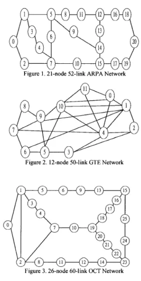
The computational experiments for the algorithms developed in Sections 3 and 4 are coded in C and performed on a PC with INTELm PII-233 CPU. We tested the algorithm for 3 networks -- ARPA, GTE, OCT with 21, 12 and 26 nodes. The network topologies are shown in Fig. 1,2 and 3.

A

Figure 2. 12-node 50-link GTE Network

Figure 3. 26-node 60-link OCT Network

The maximum number of iterations for the proposed dual Lagrangean algorithm is 1000, and the improvement counter is 30. The step size for the dual Lagrangean algorithm is initialized to be 2 and be halved of its value when the objective value of the dual algorithm, does not improve for 30 iterations. It is assumed that the traffic demand of each O-D pair is one packet per second. Unlike others’ work in [2], the candidate path set does not need to be prepared in advance and all possible candidate paths are considered for each O-D pair.

We perform two sets of computational experiments. In the first set of computational experiments, the choice of the Dw

value is fixed as to examine the solution quality of the minimum average packet delay problem.

Table 1 summarizes the results. The first column is the type of the network topology. The second column is the link

capacity. The third column is the maximum allowable end-to-end delay

(DW).

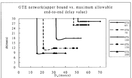
The forth column reports the lower bound of the proposed dual Lagrangean problem. The titlh column reports the upper bound of the proposed dual algorithm. The sixth column reports the error gap between the lower bound and the upper bound. The seventh column reports the maximum end-to-end delay among all O-D pairs. As can be seen in the sixth column, the gap between the lower bound and the upper bound are very tight for all different network topologies and link capacities when the value of DWis loose as compared to the maximum end-to-end delay among all O-D pairs.

Since the value for the maximum allowable end-to-end delay (DW) have a significant impact on the solution of the minimum average packet delay problem. In the second set of computational experiments, we try to examine the impact of the DW value on the solution quality of minimum average delay. Fig. 4, 5 and 6 shows the results for the ARPA, GTE, OCT network. It is clear to see that the upper bound remains almost the same with different DW value. When the Dw value below a certain threshold (as indicated in third column of Table 2), the primal solution could not be found.

Table 2 summarizes this result. The first column is the type of the network topology. The second column is the link capacity. The third column is the threshold of the maximum allowable end-to-end delay

(DW).

The forth column reports the lower bound of the proposed dual Lagrangean problem. The fifth column reports the upper bound of the proposed dual algorithm. The sixth column reports the error gap between the lower bound and the upper bound. The seventh column reports the maximum end-to-end delay among all O-D pairs. The eighth column reports the results from [2].

The maximum end-to-end delay value in the seventh column implies the optimal value for the minimax End-to-end Delay Routing problem developed in [2]. There is one thing that needs to be addressed: all possible candidate paths are considered for each O-D pair in this paper but only three candidate paths are pre-chosen for each O-D pair in [2]. Although we obtain a tighter upper bound than the minimax end-to-end delay routing problem developed in [2], this comparison is not on the same basis. On the other hand, the gap between the lower bound and the upper bound of the minimum average delay problem is still very tight, which indicate that the algorithms that we developed can achieve good system objective (average packet delay) even in stringent end-to-end delay requirements.

6. CONCLUSIONS

As compared to the work in [2], which tried to achieve better fairness among users by minimizing the maximum end-to-end delay for virtual circuit networks without considering the system perspective (minimize the average packet delay). In this paper, for the first time, we considered the problem of minimizing the average packet delay with maximum allowable end-to-end delay requirements, which indicate that we try to obtain good system performance under user’s end-to-end delay requirements.

We formulate this problem as a nonconvex and nonlinear

multicommodity integral flow problem. The nonconvex and discrete (integer constraints) properties make the problem very difficult. We take an optimization-based approach by applying the Lagrangean relaxation technique in the algorithm development. According to the computational experiments, the error gap between the upper bound and the lower bound is so tight that we can claim that a near optimal solution is found. When the maximum end-to-end delay requirements are more and more close to the threshold, the upper bound (average packet delay) remains almost the same, this indicate that this solution approach can obtain good average packet delay solution under stringent end-to-end QoS requirements.

REFERENCES

[1] B. Gavish and S. L. Hantler, “An Algorithm for Optimal Route Selection in SNA Networks,” IEEE Trans. on Cornm., COM-31, pp. 1154-1160, Oct. 1983.

[2] K. T, Cheng and F. Y. S. Lin, “Minimax End-to-End Delay Routing and Capacity Assignment for Virtual Circuit Networks,” Proc. IEEE

Globecom,pp. 2134-2138, 1995,

[3] F. Y. S. Lin and J. R. Yee, “A New Multiplier Adjustment Procedure for the Distributed Computation of Routing Assignments in Virtual Circuit Data Networks,” ORSA Journal on Computjrrg,Vol. 4, No. 3, Summer

1992.

[4] L. Kleinrock, “Queueing Systems,” Wiley-Interscience, New York, Vol. 1 and 2, 1975-1976.

[5] P. J. Corrrtois and P. Semal, “An Algorithm for the Optimization of Nonbifurcated Flows in Computer Communication Networks,” Performance EvaJuatimr, pp. 139-152, 1981.

[6] S. Chen and K. Nahrstedt, “An Overview of Quality of Service Routing for Next-Generation High-Speed Networks: Problems and Solutions,” IEEE Network,pp. 64-79, Nov.iDec. 1998,

Network topology ARPA : GTE OCT

x

-%-i-+-70 500 100 100 150 100 200 190 65 1400

i-1--E

COMPARISONOFSOLUTIONQUALITY OBTAINED BY VARIOUS NETWORKS

.ower bound (msec) Upper bound (msec) Error gap(%) Maximum end-to-end delay

I

I

I

(msec)

[

109 110.3 1.18 238.7 93.7 94,3 0.65 200.7 51.01 51.06 0.1 106.2 29.084 29.086 0.009 60.4 20.368 20.3686 0.003 42.1 28,19 28,2 0.05 50.9 26.02 26,04 0.05 46,9 17.824 17.829 0.03 31.9 11.687 11.688 0.01 20.8 8.6936 8.694 0.005 15.5 351,3 357.8 1.88 805 237.8 240.6 1.2 525.6 86,2 86.8 0.69 170.4 42.42 42.44 0.04 81.7 28,1529 28.1559 0.01 53.8

TABLE 2 – COMPARISONOF SOLUTIONQUALITY OBTAINED BY VARIOUS NETWORKSAT TrrE THRESHOLDOF MAXIMUM ALLOWABLE END-TO-END DELAY REQUIREMENTS

Network Link Threshold of D. Lower bound Upper bound Error gap (%) Maximum end-to-end Results from [2]

topology capacity (msec) (msec) (msec) delay (msec)

65 237.7 108.9 110.3 1,23 237.2 N/AT 70 203 93.6 94.4 0.9 202,2 N/A ARPA 100 110 50.7 51.2 1.02 108 NIA 150 61 28,97 29.1 0.5 60.9 NIA 200 43 20.35 20.37 0.09 42.3 NIA 65 50.88 28.17 28.23 0.2 50.876 NIA 70 47 26,026 26.046 0.08 46,9 N/A GTE 100 32 17.82 17.83 0.08 31.9 N/A 150 21.5 11,68 11.689 0.07 20.8 NIA 200 15.5 8.6 8.7 0.8 15.49 NIA 65 727 351.3 364.2 3.67 722 860.3 70 470 237.9 240.8 1.21 469.8 514.6 OCT 100 166.8 86.24 86.9 0.8 166.7 168.4 150 81.2 42.4 42.5 0.2 81.1 81.7 200 54 28,04 28.16 0.4 53,9 54.1

t: The work in [2] did not perform the computational experiments in these network settings.

ARPA network(upper bound vs. maximum allowable end-to-end delay value)

I

1 I i I I I I I I_I I — . . I I I I U I .H

o

I 1 I I I I 1 1 I

1

—

ARPA 65 — + — ARpA 70 — ARPA 100 – * – ARPA 150 — ARPA 200

0

50

100

150

200

250

300

350

400

DW(msecs)

I

Figure 4. Upper bound for different DWvalue in ARPA network

30 27 24 21 18 15 12 9 6 3 0

GTE network(upper bound vs. maximum allowable end-to-end delay value)

1 1 I I I ●s— I I I 1 ;-__.+.*. u <

0

10 20 30 40 50 60 70 Dw(msecs) —(j TE 65

1—+ ‘G,,

70 ‘GTE 100

— +

—GTE 150

Figure 5. Upper bound for different D. value in GTE network

600

500

100 0

OCT network(upper bound vs. maximum allowable end-to-end delay value)

~,

I I I I I I I I I I I I

bmm+

I I I * 1 1— — ~ 0(3 65 —* —OCI 70 + ) ‘OCT 100 —+ —ocT 150 —OCT 2(II I

750

900

0

150 300 450 600 DW(msecs)

L

‘*

I

Figure 6, Upper bound for different DWvalue in OCT network