製程能力指標Yq/Y複式抽樣之信賴下限

國立交通大學

工業工程與管理學系

碩士論文

製程能力指標

Y Y

_q

/

複式抽樣之信賴下限

Bootstrap Lower Confidence Limits for

Capability Index

Y Y

_q

/

研 究 生：林仲軒

指導教授：彭文理

博士

製程能力指標

Y Y

_q

/

複式抽樣之信賴下限

Bootstrap Lower Confidence Limits for

Capability Index

Y Y

_q

/

研究生：林仲軒

Student : Chung- Hsuan Lin

指導教授：彭文理 博士

Advisor：Dr. W. L. Pearn

國 立 交 通 大 學

工 業 工 程 與 管 理 學 系

碩 士 論 文

A Thesis

Submitted Department of Industrial Engineering and Management

College of Management

National Chiao Tung University

in partial Fulfillment of the Requirements

for the Degree of

Master

in

Industrial Engineering

December 2008

Hsinchu, Taiwan, Republic of China

中 華 民 國 九 十 八 年 六 月

製程能力指標

Y Y

_q

/

複式抽樣之信賴下限

研究生：林仲軒

指導教授：彭文理 博士

國立交通大學工業工程與管理學系碩士班

摘要

製程能力指標已廣泛被用來衡量製程的能力與產品的品質，製程良率

Y

是常見被

製造業用來判斷製程好壞的標準；品質良率

Y

則是進一步將顧客損失考慮在內。本篇

論文則是提出一個新指標

Y Y

，屏除製程不良品的部份，直接考慮顧客接收到的良

品，再計算其完全滿足顧客要求的產品比例。為一個更站在顧客角度，提供顧客更直

接判斷所接收產品好壞的指標。然而

Y Y

之估計值與其統計性質要以數學來推導表

達是非常窒礙難行，因此製程能力的檢定也就無法執行。我們運用複式抽樣，一種無

母數而大量運用電腦運算的方法來求得

Y Y

的信賴下限，以達到檢定的目的。在本

論文中介紹四種複式抽樣方法所建構的信賴下限，在五種不同母體分配（一個常態分

配與四種非常態分配）的環境下做模擬，包括對不同參數（如

Y Y

的實際值、製程

偏移程度與各分配的母體參數等）設定不同水準，做一些統整與分析，比較四種複式

抽樣信賴下限的好壞。最後也舉應用在背光模組製程的例子來說明如何使用

Y Y

指

標及複式抽樣方法求得的信賴下限，如此便可以判斷產品是否有達到原訂的水準。

關鍵字：製程能力指標、良率、品質良率、複式抽樣方法、信賴下限、模擬

Bootstrap Lower Confidence Limits for

Capability Index

Y Y

_q

/

Student : Chung- Hsuan Lin

Advisor：Dr. W. L. Pearn

Department of Industrial Engineering and Management

National Chiao Tung University

Abstract

Process capability indices are widely used in manufacturing industrial to provide a

numerical measure on whether or not a process is capable of producing items that meet

a preset quality requirement. Process yield

Y

is the most common criterion used in

the manufacturing industry for measuring process performance; Quality yield

Y

goes

a step further to take customer loss into consideration. This thesis introduce a new

index

Y Y

/

,which only considers the conformed products customer receives rather

than the proportion of non-conformed products of the manufacturing process, and

quantifies how close a product that customer has received meets 100% customer

satisfaction. The index

Y Y

/

can provide a judgment to the process from the

customer’s viewpoint. However statistical properties of the estimated

Y Y

/

are

mathematically intractable. Therefore, capability testing can not be performed. We use

a nonparametric but computer intensive method called bootstrap to obtain a lower

confidence bound on

Y Y

/

for capability testing purposes. Four types of bootstrap

lower confidence bounds are introduced and simulating for five distributions (one

normal and four non-normal) with different true values of

Y Y

/

, the degree the

process mean shifts from the target and population parameters are conducted. Then a

comparison is made of the performances of the bootstrap and the parametric estimates.

An application using the index

Y Y

/

and the bootstrap lower confidence bounds for

the backlight modules manufacturing process is presented for illustration purposes.

Keywords: Process capability indices, Yield, Quality yield, Bootstrap methods, Lower

confidence bound, Simulation.

誌謝

終於，我完成了我的論文！花了比一般人更多的時間，能完成他在過程中得到許

多人的幫助，在這一路上有著許多人的幫助與支持。首先，謝謝彭文理老師，從老師

身上學到了對於學術研究的嚴謹態度，適時的提點我思考方向；謝謝吳建瑋學長，即

使已經到台中任教，仍不辭辛勞的指導我。

在同一個實驗室的大家，很幸運能認識你們，日常生活中長時間的相處，一起吃

飯、聊天、打球的時光即使簡單，不過這也是我最喜歡的。當然，寫論文當中所遇到

的統計或者程式上各種問題，也多虧了有你們的協助，才能解決進而完成論文。謝謝

啦！mb517！

謝謝我的幾位好朋友，在不同地方認識的你們，也許身處各地，但都會偶爾來電

關心，偶爾見個面，唱個歌聊聊近況，最重要的是不斷的給我鼓勵。謝了，好友們！

最後，感謝我親愛的家人，爸媽無微不至的照顧與包容，雖然不在身邊，他們的

用心讓我不管在經濟或是身心都能無後顧之憂。我知道他們一直擔心我，卻從不給我

壓力。老爸老媽，謝了！還有姐姐與姐夫因為也在新竹，會就近照顧我，常常找我到

家裡打牙祭，更貼心的給我許多鼓勵與建議。親愛的老姊，謝謝妳總在我迷惘的時候

引導我。說感謝也許還不夠，期待自己用行動回報你們。

還有曾經陪伴我十年的妳，謝謝妳。

Content

摘要

... i

Abstract

... ii

誌謝

... iii

Content

...iv

List of Tables

...v

List of Figures

...vii

1. Introduction

...1

1.1. Motivation ...1

1.2. Purpose ...1

1.3. Structure...2

2. Literature Review

...3

2.1. Process Capability Indices...3

2.2. Lower Confidence Limits for Capability Indices ...4

2.3. Process Yield

Y

and Quality Yield

Y

...4

3. The Index

Y Y

/

...7

3.1. Definition and Interpretation of the Index

Y Y

/

...7

3.2. Estimation of the Index

Y Y

/

...9

4. Bootstrap Resampling Methods

...11

4.1. The Bootstrap Methodology...11

4.1.1. Standard Bootstrap (SB)...12

4.1.2. The Percentile Bootstrap (PB) ...13

4.1.3. Biased-corrected Percentile Bootstrap (BCPB) ...13

4.1.4. Bootstrap-t (BT)...13

4.2. The Simulating Method ...14

5. The Procedures and Analysis of the Simulations

...15

5.1. Simulation Analysis for Normally Distributed Process...15

5.2. Simulation Analysis for Student’s t Process ...18

5.3. Simulation Analysis for Chi-squared Process ...22

5.4. Simulation Analysis for Gamma Process ...25

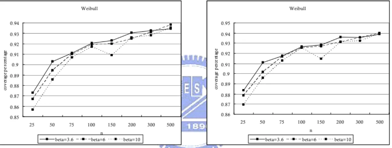
5.5. Simulation Analysis for Weibull Process ...28

5.6. Average Bounds ...32

6. Application Examples

...34

6.1. An application for BLM...34

6.2. Data Analysis...35

7. Conclusions

...38

References

...39

Appendix A

. ...41

Appendix B

. ...47

List of Tables

Table 1. Values of the two indices for normal processes with various , fixed 

1

and



LSL T USL

, ,

 

 

3,0,3



. ... 8

Table 2. Coverage percentages for the 95% bootstrap lower confidence limits for

normal process with 

 0

T

,

USL 

3

and

LSL 

3

. ...16

Table 3. Coverage percentages for the 95% bootstrap lower confidence limits for

Student’s t process with 

 0

T

and degrees of freedom

k

3

...19

Table 4. Coverage percentages for the 95% bootstrap lower confidence limits for

Chi-squared process with 

 

T

12 and degrees of freedom

k

12

. ...23

Table 5. Numbers of 120 groups coverage percentages decrease as the true values of

/

Y Y

increase with each sample size n for Chi-squared process...23

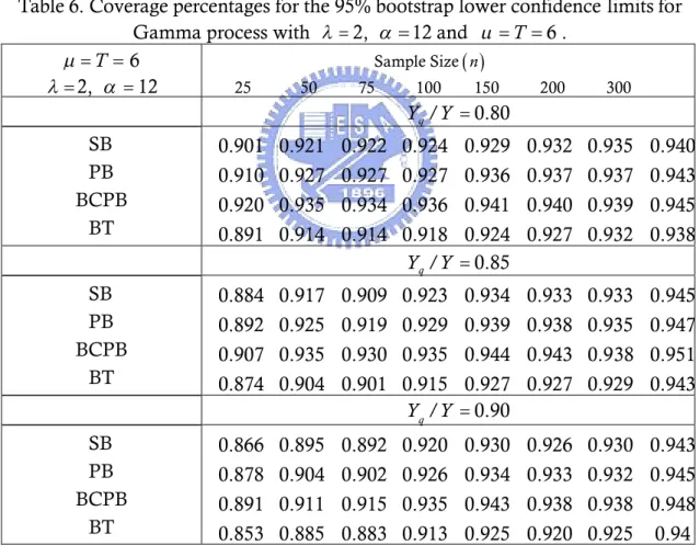
Table 6. Coverage percentages for the 95% bootstrap lower confidence limits for

Gamma process with 



2, 12 and 

 

T

6 . ...26

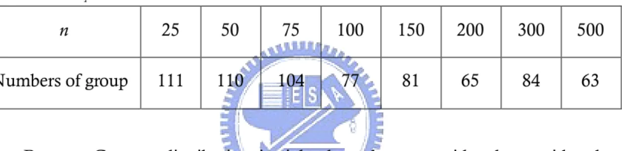
Table 7. Numbers of 120 groups coverage percentages decrease as the true values of

/

Y Y

increase with each sample size n for Gamma process...28

Table 8. Coverage percentages for the 95% bootstrap lower confidence limits for

Weibull process with 10, 



10 and 

T

...29

Table 9. Numbers of 120 groups coverage percentages decrease as the true values of

/

Y Y

increase with each sample size n for Weibull process. ...31

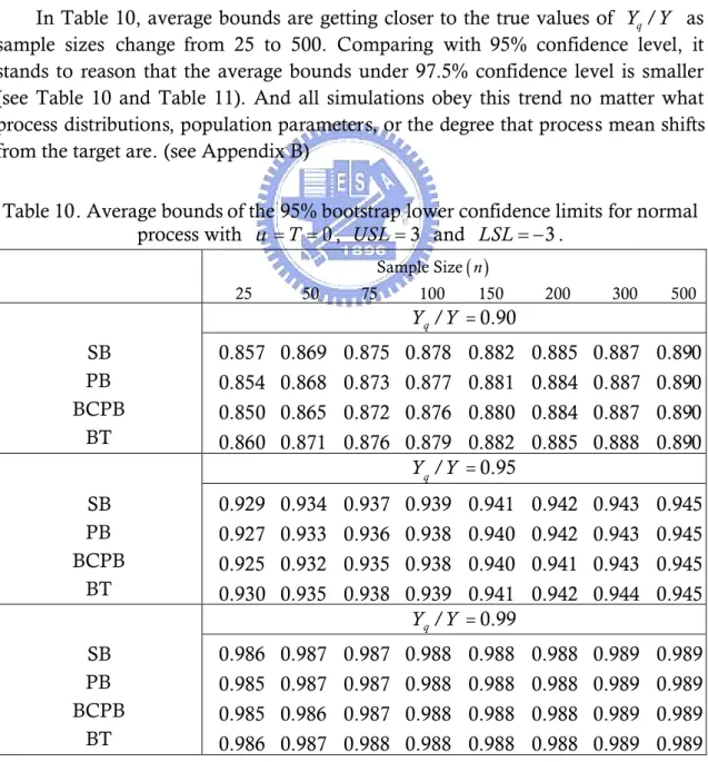
Table 10. Average bounds of the 95% bootstrap lower confidence limits for normal

process with 

 0

T

,

USL 

3

and

LSL 

3

. ...32

Table 11. Average bounds of the 97.5% bootstrap lower confidence limits for normal

process with 

 0

T

,

USL 

3

and

LSL 

3

. ...33

Table 12. 100 samples of length from historical data. ...35

Table 13. 100 samples of luminance from historical data. ...35

Table 14. Four bootstrap lower confidence bounds of

Y Y

/

for the data in Table 12.

...37

Table 15. Four bootstrap lower confidence bounds of

Y Y

/

for the data in Table 13.

...37

Table 16. Values of parameters under normal process.. ...41

Table 17. Values of parameters under Student’s t process. ...41

Table 18. Values of parameters under Chi-squared process ...42

Table 19. Values of parameters under Gamma process. ...43

Table 20. Values of parameters under Weibull process ...45

Table 21A(B). Average bound and coverage percentage of 95%(97.5%) bootstrap for

normal process with

T

0

,

USL

3

,

LSL

3

. ...47

Table 22A(B). Average bound and coverage percentage of 95%(97.5%) bootstrap for

Student’s t process with 

0

,

k

3

...48

Table 23A(B). Average bound and coverage percentage of 95%(97.5%) bootstrap for

Student’s t process with 

0

,

k

10

. ...50

Table 24A(B). Average bound and coverage percentage of 95%(97.5%) bootstrap for

Student’s t process with 

0

,

k

20

. ...51

Table 25A(B). Average bound and coverage percentage of 95%(97.5%) bootstrap for

Chi-squared process with 

0

,

k

12

. ...53

Table 26A(B). Average bound and coverage percentage of 95%(97.5%) bootstrap for

Chi-squared process with 

0

,

k

15

...55

Table 27A(B). Average bound and coverage percentage of 95%(97.5%) bootstrap for

Chi-squared process with 

0

,

k

20

. ...58

Table 28A(B). Average bound and coverage percentage of 95%(97.5%) bootstrap for

Gamma process with 

12

, 

2

,   

 /

. ...60

Table 29A(B). Average bound and coverage percentage of 95%(97.5%) bootstrap for

Gamma process with 

15

, 

2

,   

 /

. ...63

Table 30A(B). Average bound and coverage percentage of 95%(97.5%) bootstrap for

Gamma process with 

20

, 

2

,   

 /

...65

Table 31A(B). Average bound and coverage percentage of 95%(97.5%) bootstrap for

Weibull process with 

10

, 

3.6

,





1

 



 

. ...68

Table 32A(B). Average bound and coverage percentage of 95%(97.5%) bootstrap for

Weibull process with 

10

, 

6

,

 







 

. ...70

Table 33A(B). Average bound and coverage percentage of 95%(97.5%) bootstrap for

Weibull process with 

10

, 

10

,





1

 



List of Figures

Figure 1. Values of the two indices for normal processes with various , fixed 

1

and



LSL T USL

, ,

 

 

3,0,3



. ... 9

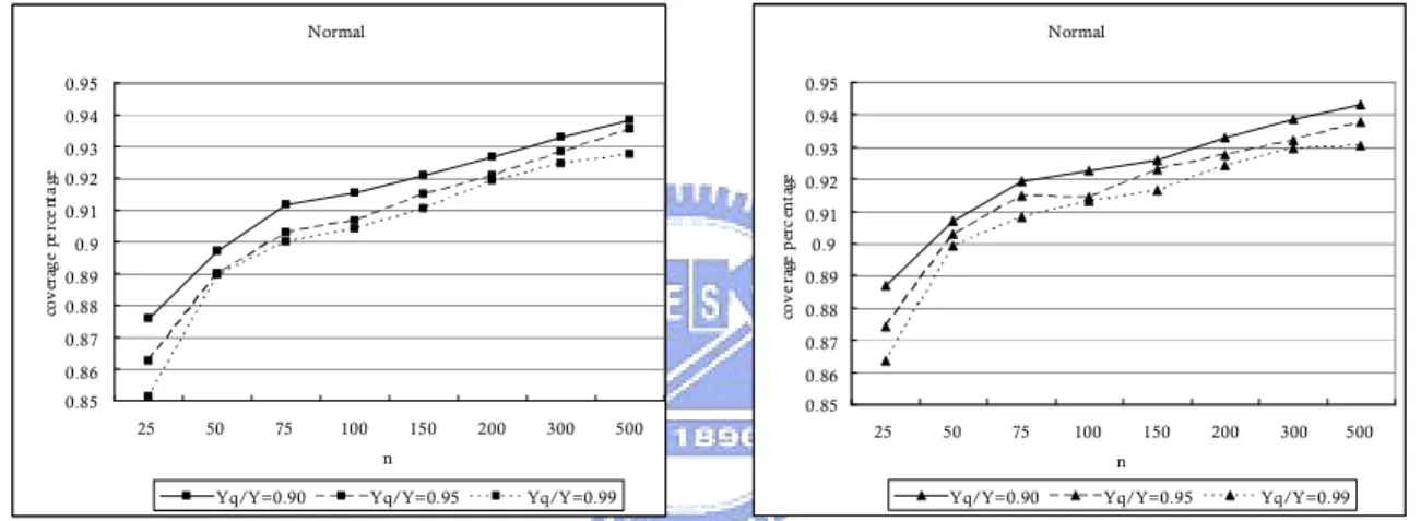
Figure 2. Coverage percentages for the 95% bootstrap lower confidence limits for

normal process with true value of

Y Y 

/

0.90

,



 

T

0

,

USL 

3

, and

3

LSL 

. ...17

Figure 3. Coverage percentages for the 95% bootstrap lower confidence limits for

normal process with true value of

Y Y 

/

0.95

,



 

T

0

,

USL 

3

, and

3

LSL 

. ...17

Figure 4. Coverage percentages for the 95% SB lower confidence limits for normal

process with



 

T

0

,

USL 

3

, and

LSL 

3

. ...17

Figure 5. Coverage percentages for the 95% SB lower confidence limits for normal

process with



 

T

0

,

USL 

3

, and

LSL 

3

. ...17

Figure 6. Coverage percentages for the 95% SB lower confidence limits for normal

process with true value of

Y Y 

/

0.90

,

USL 

3

, and

LSL 

3

. ...17

Figure 7. Coverage percentages for the 95% PB lower confidence limits for normal

process with true value of

Y Y 

/

0.90

,

USL 

3

, and

LSL 

3

. ...17

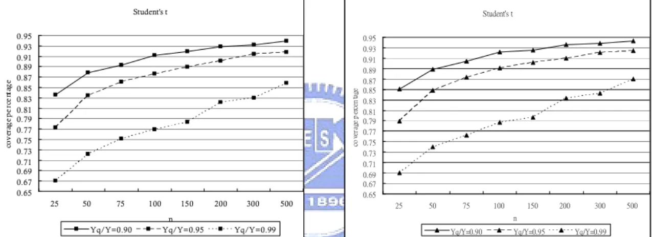
Figure 8. Coverage percentages for the 95% bootstrap lower confidence limits for

Student’s t process with

k 

3

,



 

T

0

, and true value of

Y Y 

/

0.90. ...20

Figure 9. Coverage percentages for the 95% bootstrap lower confidence limits for

Student’s t process with

k 

3

,



 

T

0

, and true value of

0.95. ...20

Figure 10. Coverage percentages for the 95% SB lower confidence limits for Student’s t

process with



 

T

0

, and

k 

3

. ...20

Figure 11. Coverage percentages for the 95% PB lower confidence limits for Student’s t

process with



 

T

0

, and

k 

3

. ...20

Figure 12. Coverage percentages for the 95% SB lower confidence limits for Student’s t

process with true value of

Y Y 

/

0.90

, and

k 

3

. (mu=μ)...20

Figure 13. Coverage percentages for the 95% PB lower confidence limits for Student’s t

process with true value of

Y Y 

/

0.90

, and

k 

3

. (mu=μ)...20

Figure 14. Coverage percentages for the 95% SB lower confidence limits for different

Student’s t processes (d.f.=3, 4 and 5) and normal process with



 

T

0

and

true value of

Y Y 

/

0.90

.. ...21

Figure 15. Coverage percentages for the 95% PB lower confidence limits for different

Student’s t processes (d.f.=3, 4 and 5) and normal process with



 

T

0

and

true value of

Y Y 

/

0.90

.. ...21

Figure 16. Coverage percentages for the 95% SB lower confidence limits for different

Student’s t processes (d.f.=3, 4 and 5) and normal process with



 

T

0

and

true value of

Y Y 

/

0.95

.. ...21

Figure 17. Coverage percentages for the 95% PB lower confidence limits for different

Student’s t processes (d.f.=3, 4 and 5) and normal process with



 

T

0

and

true value of

Y Y 

/

0.95

. ...21

Figure 18. Coverage percentages for the 95% SB lower confidence limits for different

Student’s t processes (d.f.=3, 4 and 5) and normal process with



 

T

0

and

true value of

Y Y 

/

0.99

...21

Figure 19. Coverage percentages for the 95% PB lower confidence limits for different

Student’s t processes (d.f.=3, 4 and 5) and normal process with



 

T

0

and

true value of

Y Y 

/

0.99

...21

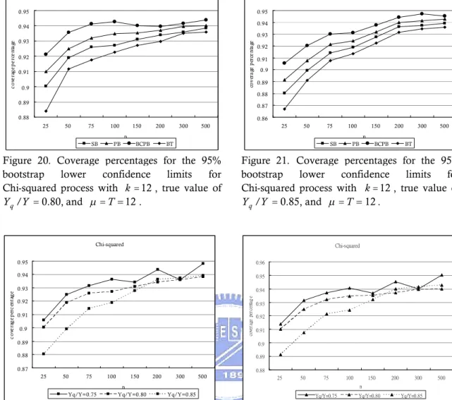
Figure 20. Coverage percentages for the 95% bootstrap lower confidence limits for

Chi-squared process with

k 

12

, true value of

Y Y 

/

0.80, and



 

T

12

. ..24

Figure 21. Coverage percentages for the 95% bootstrap lower confidence limits for

Chi-squared process with

k 

12

, true value of

Y Y 

/

0.85, and



 

T

12

. ..24

Figure 22. Coverage percentages for the 95% SB lower confidence limits for

Chi-squared process with

k 

12

, and



 

T

12

. ...24

Figure 23. Coverage percentages for the 95% PB lower confidence limits for

Chi-squared process with

k 

12

, and



 

T

12

. ...24

Figure 24. Coverage percentages for the 95% SB lower confidence limits for

Chi-squared process with

k 

12

, and true value of

Y Y 

/

0.75. ...24

Figure 25. Coverage percentages for the 95% PB lower confidence limits for

Chi-squared process with

k 

12

, and true value of

Y Y 

/

0.75. ...24

Figure 26. Coverage percentages for the 95% SB lower confidence limits for

Chi-squared process with true value of

Y Y 

/

0.75, and





T

. ...25

Figure 27. Coverage percentages for the 95% PB lower confidence limits for

Chi-squared process with true value of

Y Y 

/

0.75, and





T

. ...25

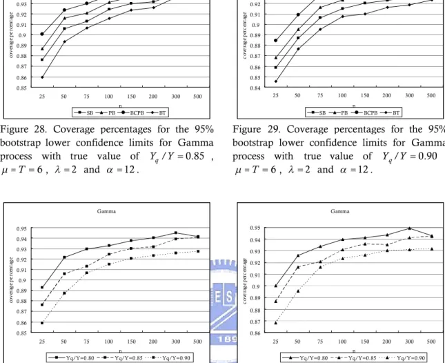
Figure 28. Coverage percentages for the 95% bootstrap lower confidence limits for

Gamma process with true value of

Y Y 

/

0.85

,



 

T

6

,





2

and





12

.

...27

Figure 29. Coverage percentages for the 95% bootstrap lower confidence limits for

Gamma process with true value of

Y Y 

/

0.90

,



 

T

6

,





2

and





12

.

...27

Figure 30. Coverage percentages for the 95% SB lower confidence limits for Gamma

process with



 

T

6

,





2

and





12

...27

Figure 31. Coverage percentages for the 95% PB lower confidence limits for Gamma

process with



 

T

6

,





2

and





12

...27

Figure 32. Coverage percentages for the 95% SB lower confidence limits for Gamma

process with the true value of

Y Y 

/

0.80

,





2

and





12

. ...27

Figure 33. Coverage percentages for the 95% PB lower confidence limits for Gamma

Figure 34. Coverage percentages for the 95% SB lower confidence limits for Gamma

process with the true value of

Y Y 

/

0.80

,





2

and





T

(alpha 

 )...28

Figure 35. Coverage percentages for the 95% PB lower confidence limits for Gamma

process with the true value of

Y Y 

/

0.80

,





2

and





T

(alpha





T

).28

Figure 36. Coverage percentages for the 95% bootstrap lower confidence limits for

Weibull process with the true value of

Y Y 

/

0.80

,





10

,





10

and





T

.

...30

Figure 37. Coverage percentages for the 95% bootstrap lower confidence limits for

Weibull process with the true value of

Y Y 

/

0.85

,





10

,





10

and





T

.

...30

Figure 38. Coverage percentages for the 95% SB lower confidence limits for Weibull

process with





10

,





10

and





T

...30

Figure 39. Coverage percentages for the 95% PB lower confidence limits for Weibull

process with





10

,





10

and





T

...30

Figure 40. Coverage percentages for the 95% SB lower confidence limits for Weibull

process with the true value of

Y Y 

/

0.80

,





10

and





10

. ...31

Figure 41. Coverage percentages for the 95% PB lower confidence limits for Weibull

process with the true value of

Y Y 

/

0.80

,





10

and





10

...31

Figure 42. Coverage percentages for the 95% SB lower confidence limits for Weibull

process with the true value of

Y Y 

/

0.90

,





10

and





T

...31

Figure 43. Coverage percentages for the 95% PB lower confidence limits for Weibull

process with the true value of

Y Y 

/

0.90

,





10

and





T

...31

Figure 44. Average bounds for the 95% bootstrap lower confidence limits for normal

process with true value of

Y Y 

/

0.90

,



 

T

0

,

USL 

3

, and

LSL 

3

...33

Figure 45. Average bounds for the 97.5% bootstrap lower confidence limits for normal

process with true value of

Y Y 

/

0.90

,



 

T

0

,

USL 

3

, and

LSL 

3

...33

Figure 46. The structure of backlight module...34

Figure 47. Specification of length for the assemble frame of BLM...34

Figure 48. The histogram plot for the data of Table 12...36

1. Introduction

1.1. Motivation

Process capability indices (PCIs) are used to measure process performance by

considering process location, process variation, and manufacturing specifications.

In the late 1980’s and the early 1990’s, techniques and tables were developed to

construct lower confidence limits for process indices

C

、

C

and

C

because

decision makers would prefer a lower bound on process capability indices to the

sample point estimate. However, these techniques assume that the underlying

process is normally distributed.

Process yield

Y

is the most common criterion used in the manufacturing

industry, and Ng and Tsui (1992) proposed a more customer-oriented measure of

yield, which is referred to as quality yield

Y

. Process yield

Y

and quality yield

q

Y

have the advantage that the formula can be applied to process with arbitrary

distribution. Unfortunately, statistical properties of the estimated

Y

are

mathematically intractable.

In order to overcome those problem, a nonparametric but computer intensive

method called bootstrap is used to obtain lower confidence bounds on

C

、

C

and

pm

C

by Franklin and Wasserman (1992) and on

Y

by Pearn et al. (2005) for

capability estimation purposes.

The index

Y

is more customer-oriented measure of yield, but there is another

index

Y Y

/

, which is quality yield divided by yield is rarely mentioned. Ng and

Tsui (1992) mentioned:

Y

is the manufacturing yield while

Y Y

/

can be

considered the customer ”yield”. This statement motivates one to consider whether

the index

Y Y

/

is more customer-oriented than

Y

. In the past many researches

discussed process capability indices from manufacturers’ viewpoint. But now

customers’ thought is more emphasized, we can try to do some studies on the

index.

Process yield

Y

is defined as the percentage of the processed product units

passing the inspections; quality yield

Y

can be expressed as the percentage of the

processed product units that are really satisfactory to the customer. But one

customer may be not interested in process yield

Y

because of whatever

Y

is, the

customer will just take the production units those passed the inspection. Customer

always wishes each unit he receive from his vender is 100% satisfied, the index

/

q

Y Y

can be considered the customer ”yield” may measure probability more

customer-oriented than

Y

.

1.2. Purpose

The purposes of this thesis are as follows: First, we interpret the difference

between the indices

Y Y

/

and

Y

including distinguish their performance in

different scenario and find the advantage of

Y Y

/

. Second, the bootstrap

resampling method is used to obtain four kinds of bootstrap lower confidence

bounds on the index

Y Y

/

for capability testing purpose. The lower confidence

bounds can be utilized to perform quality testing and measure if the process can

reproduce product items which are in the specifications. Finally, we analyze these

bootstrap confidence limits’behavior for processes of normal, skewed (Chi-Squared,

Gamma and Weibull), and heavy tailed (Student’s t) distributions, and a

comparison is made of the performances of the bootstrap and the parametric

estimates.

1.3. Structure

In Chapter 1, the motivation and the purpose of this thesis are presented. The

literature reviews are presented in Chapter 2, including an introduction of the four

basic process capability indices

C

、

C

、

C

and

C

, the definitions of process

yield

Y

, quality yield

Y

, and some lower confidence limits for capability indices.

In Chapter 3, we give a definition on the index

Y Y

/

and then the sample

estimator of

Y Y

/

is made. In Chapter 4, we introduce the bootstrap estimation

method and the definitions of the four bootstrap confidence intervals. Then we

introduce how to execute the simulations. In Chapter 5 we show the results and

analysis of the simulations. For illustrating purpose, an application of

manufacturing process is presented in Chapter 6. We made some conclusions in

Chapter 7.

2. Literature Review

Process capability indices are intended to provide single-number assessments

of ability to meet specification limits on quality characteristics (Kotz and Johnson

(2002)). It has been proposed in the manufacturing industry to measure on whether

a process is capable of reproducing items or not. A review in this section is going to

describe some and current development in PCIs.

2.1. Process Capability Indices

Many authors have promoted the use of various PCIs for evaluating a process’s

capability. Examples include Boyles (1991), Pearn et al. (1992), Kushler and Hurley

(1992), Kotz and Lovelace (1998), Pearn et al. (1998), Kotz and Johnson (2002),

Pearn and Shu (2003) and references therein. The first process capability index

appearing in literature was the precision index

C

and defined as (see Juran (1974)

and Kane (1986)):







6

USL LSL

C

,

where

USL

is the upper specification limit,

LSL

is the lower specification limit,

and  is the process standard deviation. The index

C

measures process

precision (product quality consistency), which does not consider whether the

process is centered.

The

C

index considers process variation and the location of process mean;

defined as (see Juran (1974) and Kane (1986)):

 















_

_





min

,

3

3

USL

LSL

C

_,

where  is the process mean.

Taguchi, on the other hand, emphasizes the product loss when one of its

characteristics departs from the target value

T

. Hsiang and Taguchi (1985)

introduced the index

C

, which was also proposed independently by Chan et al.

(1988). The index

C

incorporates with the variation of production items with

respect to the target value and the specification limits preset in the factory. It is

defined as:













 

6

USL LSL

C

T

.

The fourth well-known capability index is

C

index Pearn et al. (1992). It

considers both on the advantage of

C

and

C

, it is defined as:























_

_









_

_



 

 







min

,

3

3

USL

LSL

C

T

T

.

2.2. Lower Confidence Limits for Capability Indices

Chou et al. (1990) provided tables for constructing 95% lower confidence limits

for both

C

and

C

. Their tables for limits on

C

, however, are conservative and

an approximation presented by Bissell (1990) is recommended instead (see Franklin

and Wasserman (1992) and Kushler and Hurley (1992)). Finally, Boyles (1991)

provided an approximate method for finding lower confidence limits for

C

.

All of the calculation for these lower confidence limits have an assumption that

the processes are normally distributed, but many real world processes are not (see

Gunter (1989)), and this departure from normality may be hard to detect. This

could potentially affect both the estimates of the indices and the lower confidence

limits based on these estimates. Efron (1979, 1982) introduced the nonparametric

estimation method called bootstrap, Four types of bootstrap confidence intervals,

including the standard bootstrap confidence interval (SB), the percentile bootstrap

confidence interval (PB), the biased corrected percentile bootstrap confidence

interval (BCPB), and the bootstrap-t (BT) method introduced by Efron (1981) and

Efron and Tibshirani (1986) was conducted in this research. Franklin and

Wasserman (1992) investigated the lower confidence bounds for the capability

indices,

C

,

C

and

C

using the first three bootstrap methods. Some

simulations were conducted and a comparison was made among the three bootstrap

methods based on the parametric estimates. The procedures of simulations are

presented in section 4.2.

The simulation results indicate that for normal processes the bootstrap

confidence limits perform equally well as results obtained by Chou et al. (1990),

Bissell (1990), and Boyles (1991). And for non-normal processes the bootstrap

estimates performed significantly better than other methods.

2.3. Process Yield

Y

and Quality Yield

Y

Traditionally, process yield

Y

is defined as the percentage of the processed

product units passing the inspections, which has for a long time been the most

common and standard criteria used in the manufacturing industries for judging

process performance. According to the manufacturing specifications placed on

various key product characteristics, units are inspected and sorted into two

categories: accepted (conforming items) and rejected (defectives). For product units

rejected during the inspection, additional costs would be incurred to the factory for

scrapping or reworking. All passed product units are treated equally and accepted

by the producer. No additional cost to the factory is required. The definition of

Y

index is





_

LSL

where

USL

and

LSL

are the upper and lower specification limits, respectively,

and

F x is the cumulative distribution function of the measured characteristic



X

. The disadvantage of yield measure is that it does not distinguish the products

that fall inside of the specification limits. Customers do notice unit-to-unit

differences in these characteristics, especially if the variance is large and/or the

mean is offset from the target. To rectify this, a more accurate, complete and

customer-oriented measure of yield, which is referred to as quality yield

Y

(Q-yield), was proposed by Ng and Tsui (1992). The index distinguishes the

products within the specifications by increasing the penalty as the departure from

the target increases. The quadratic loss function is incorporated with the yield

measure. Johnson (1992) developed the relative expected loss

L to provide

comparisons between processes, defined as:

 

_



_



 













x T

L

dF x

d

,

where 

_{is the process variance,  is the process mean,}

_T

_{is the target value}

and

d





USL LSL





2

is the half specification width. The disadvantage of the

L

index is the difficulty in setting a standard for the index since it increases from zero

to infinity. The quality yield index

Y

differs from the expected relative worth

index defined by Johnson (1992) by truncating the deviation outside the

specifications. With this truncation, the quality yield index will be between zero and

one and thus has better interpretation.

The main idea of the quality yield index

Y

is that it penalizes the yield

measure for the variation of the product characteristics from its target. It was

suggested by Ng and Tsui (1992) by connecting the proportion-conforming-based

index

Y

and loss-function-based index

L . Unlike the process yield

Y

, the

quality yield

Y

focuses on the ability of the process to cluster around the target by

taking the relative loss within the specifications into consideration. If the

USL

and

LSL

are the upper and lower specification limits, respectively,

T

is the target

value,

d

is the half specification width, and

F x



is the cumulative distribution

function of the measured characteristic, then the index

Y

is defined as:

 

_



_





















1

x T

Y

dF x

d

,

Pearn et al. (2005) described the advantage of using the index

Y

. Quality yield can

be treated as traditional yield minus truncated expected relative process loss within

the specifications, which produces a way to quantify how well a process can meet

customer requirements. While yield is the proportion of conforming products,

quality yield can be interpreted as the proportion of “perfect” products. By relating

to the yield measure, which is familiar to engineers, it is much easier for the

engineers to understand and accept this capability measure. The advantage of the

index over the

L index is that the value of the former goes from zero to one.

Similarly to the yield index, the

Y

measure, the ideal value of

Y

is one, which

provides the user a clear concept about the standard. Similar to

Y

, the index

Y

does not rely on the normality assumption. Current practices of measuring

manufacturing capability by only evaluating the point estimates of capability indices

have been severely criticized since it ignores sampling error. The sampling

distribution and sampling errors of the estimated quality yield have never been

investigated due to their mathematical intractability. A decision maker, however,

may be interested in the lower confidence bound on the quality yield rather than

just the point estimate, which does not convey reliable information. Pearn et al.

(2005) applied the bootstrap method to construct lower confidence bounds of index

q

3. The Index

Y Y

/

3.1. Definition and Interpretation of

the Index

Y Y

/

Given the definitions of process yield

Y

and quality yield

Y

, the index

/

q

Y Y

can be defined to be:



_{ }

_



_























/

1

x T

Y Y

dF x

dF x

d

,

The process yield

Y

measures the percentage of processed units that pass

inspection and customers only accept those passed units, called conforming

products. The index

Y

takes customer loss into consideration which measures

Y

minus the truncated expected relative process loss within the specifications. The

index

Y

can be viewed as the percentage of process units are perfect products.

The meaning of

Y

divided by

Y

is the proportion of “passed” units that can be

viewed as perfect products.

The process yield

Y

can be treated as the satisfaction level of manufacturers.

Use of field as a quality measure implies that each passed unit costs the

manufacturers nothing additional but each rejected unit costs the factory an

additional amount for scraping or repairing it. Therefore the higher process yield is,

the less cost should be paid. For that reason, manufacturers just focus on the

percentage of processed units those pass inspection. However, passed units have

different distance toward target of the specifications in any characteristic.

Considering that customers do notice unit-to-unit differences,

Y

is proposed to

provide a more customer-oriented index to remedy this disadvantage. In contrast,

customers would not regard process yield

Y

as much as the manufacturers do,

whatever the process yield is, customers always accept conformed products.

Taking the two problems into consideration, we analyze the similarities and

differences between the indices

Y

and

Y Y

/

. We also evaluate their advantages,

weaknesses, and the performance with different parameter setting.

Customers receive conformed units regardless what the index

Y

is, quality

yield divided by yield indicates this index considering products within the

specifications. The index

Y Y

/

represents the percentage of conformed units

equal to 100% customer satisfaction.

Because the index

Y Y

/

is a combination of

Y

and

Y

, the index

Y Y

/

have some same advantages with

Y

. First, the index

Y Y

/

does not rely on the

normal distribution assumptions. Second, the value of

Y Y

/

goes from zero to

one, the ideal value of

Y Y

/

is one, providing a clear standard. Finally, the

index

Y Y

/

is also flexible because it compares the quality of different

characteristics of a product on a single percentage scale.

For instance, case 1 : if

Y



0.9,

Y



0.7, then

Y Y

/



77.8%

case 2 : if

Y



0.5,

Y



0.45, then

Y Y

/



90%

In case 1 both of

Y

and

Y

are larger than those in case 2, but the value of

/

q

Y Y

in case 1 is smaller. The different results from considering process product

units or only conformed units.

Table 1. Values of the two indices for normal processes with various

, fixed 

1

and



LSL T USL

, ,

 

 

3,0,3



.



Y

Y Y

/

-3.0

0.210405964821687

0.42081193047371

-2.8

0.262303242443558

0.452824941335896

-2.6

0.31944841741512

0.487393692272008

-2.4

0.380565100962162

0.524377200567277

-2.2

0.44410368098257

0.563480021726843

-2.0

0.508359216331457

0.604222456856418

-1.8

0.571595823442333

0.645922415173605

-1.6

0.632159202348002

0.687696746923721

-1.4

0.688563462990348

0.728488034252458

-1.2

0.739545146765709

0.767118185743577

-1.0

0.784084322686022

0.802363612594988

-0.8

0.821398208972198

0.833040614288525

-0.6

0.850916012177887

0.858086738010264

-0.4

0.872244513964856

0.876625993499298

-0.2

0.885132937401514

0.888012110890559

0.0

0.88944363577395

0.891851452815273

0.2

0.885132937401514

0.888012110890559

0.4

0.872244513964856

0.876625993499298

0.6

0.850916012177887

0.858086738010264

0.8

0.821398208972198

0.833040614288525

1.0

0.784084322686022

0.802363612594988

1.2

0.739545146765709

0.767118185743577

1.4

0.688563462990348

0.728488034252458

1.6

0.632159202348002

0.687696746923721

1.8

0.571595823442333

0.645922415173605

2.0

0.508359216331457

0.604222456856418

2.2

0.44410368098257

0.563480021726843

2.4

0.380565100962162

0.524377200567277

2.6

0.31944841741512

0.487393692272008

2.8

0.262303242443558

0.452824941335896

3.0

0.210405964821687

0.42081193047371

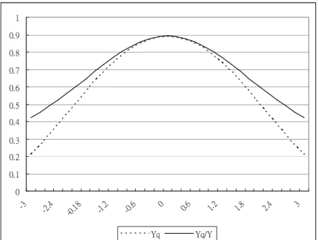
Figure 1. Values of the two indices for normal processes with various , fixed



1

and



LSL T USL

, ,

 

 

3,0,3



.

Table 1 displays values of the indices

Y

and

Y Y

/

using normal processes

for various values of  with fixed 

1

, and



LSL T USL

, ,

 

 

3,0,3



. Figure 1

plots those data in Table 1.  is varied from -3 to 3 in unit steps to examine the

sensitivity of the indices

Y

and

Y Y

/

with respect to . For the symmetric

case, the two indices obtain their maximum at 

T

. However, as  departs

from

T

, two indices decrease and

Y Y

/

decreases slower than

Y

.

3.2. Estimation of the Index

Y Y

/

In practical applications, sample data must be collected to estimate the index.

Suppose

X ,

X , . . .,

X

denote the sample measurements of product

characteristics. A natural estimator of

Y

and

Y

may be expressed as:

 





1

ˆ

Y

n

,







_{ }



















1

ˆ

x T

d

Y

n

,

according to the definition of

Y Y

/

, so that the estimator of

Y Y

/

may be

expressed as:



ˆ

c

Y

Y

ˆ /

Y

ˆ

,

where ˆ

Y represent estimated

Y Y

/

for the purpose of easily displaying. So

 /

c q

Y

Y Y

and we use

Y to represent the index

Y Y

/

in some places. In

addition to point estimation, however, a decision maker may be interested in a

0 0.1 0.2 0.3 0.4 0.5 0.6 0.7 0.8 0.9 1 -3 _-2.4 -0.18 -1.2 -0.6 0 0.6 1.2 1.8 2.4 3 Yq Yq/Y

lower limit on the quality yield divided by yield from the process as well. The

sampling distribution of ˆ

Y is then required, but unfortunately, the derivation of

the exact distribution of ˆ

Y is mathematically intractable. Pearn et al. (2004)

constructed an approximate lower confidence bound of the estimator ˆ

Y for very

low fraction of defectives under the assumption of normality. However, the

calculation of the approximation is rather messy and cumbersome to undertake.

Further, the accuracy of the approximation has not been investigated. Compared

with the ˆ

Y , the ˆ

Y is more complicated so that the derivation of the exact

distribution of ˆ

Y is mathematically intractable. A nonparametric method called

4. Bootstrap Resampling Methods

4.1. The Bootstrap Methodology

Traditionally, statistical research work has relied on the central limit theorem

and normal approximations to obtain standard errors and confidence intervals.

These techniques are valid only when the statistic, or some known transformation

of the statistic, is asymptotically normally distributed. Unfortunately, many real

world processes are not normally distributed and this departure from normality

could potentially affect these estimates. A major motivation for the traditional

reliance on normal-theory methods has been computational tractability. Access to

powerful computation enables the use of statistics in new and varied ways.

Idealized models and assumptions can now be replaced with more realistic

modeling or by virtually model-free analyses. Much statistical work and data

analysis is undertaken today by computers in ways that are too complicated for

practical analytical treatment. The new effects of these computational advances are

probably best reflected in the recent enormous success of bootstrap methodology,

which shows that many problems, previously difficult to solve, can be conquered.

For either normal or non-normal distributions, the bootstrap method could be

applied to return valid inferential results required.

The essence of bootstrapping is the idea that in the absence of any other

knowledge about a population, the distribution of values found in a random sample

of size n from the population is the best guide to the distribution in the population.

By resampling observations from the observed data, the process of sampling

observations from the population is mimicked. Instead of using a sample statistic to

estimate a population parameter, as is done within the framework of conventional

parametric statistical tests, the bootstrap uses multiple samples derived from the

original data to provide what in some instances may be a more accurate measure of

the population parameter. Therefore, to approximate what would happen if the

population was resampled, it is sensible to resample the sample. In other words, the

infinite population that consist of the n observed sample values, each with

probability

1/ n

, is used to model the unknown real population. The sampling is

with replacement, which is the only difference in practice between bootstrapping

and randomization in many applications.

The bootstrap, a data-based simulation technique for statistical inference is a

nonparametric, computationally intensive but effective estimation method. The

most common application of the bootstrap involves estimating a population

standard error and/or confidence interval. In particular, one can use the sampling

distribution of a statistic, while assuming that the sample is only representative of

the population from which it is drawn, and that the observations are independent

and identically distributed. The main merit of the nonparametric bootstrap is that it

does not rely on any distributional assumptions about the underlying population.

The more ambiguous the information is to the researcher regarding the underlying

population distribution, the more likely it is that the bootstrap may prove useful.

Rather than using distribution frequency tables to compute approximate p

probability values, the bootstrap method generates a unique sampling distribution

based on the actual sample rather than the analytic methods. The formulation detail

follows.

In this method,

B

new samples, each of the same size as the observed data,

are drawn with replacement from the available sample. The statistic of interest is

then calculated for each new set of resampled data, in our case say,

1

ˆ

Y ,

ˆ

Y ,… ,

ˆ

Y ,

yielding a bootstrap distribution for the statistic, say

Y . Assume the

ˆ

observations

x ,

x ,… ,

x to be a random sample of size n taken from a process. A

bootstrap sample, denoted by

x

,

2

x

,… ,

n

x

is a sample of size n drawn with

replacement from the original sample. There are possibly a total of

_n

_such

resamples. Each such sample is called a “bootstrap sample.” In our case, these

resamples would then be used to calculate

_n

_{values of}

ˆ

c

Y . Each of these would

be an estimate of

Y and the entire collection would constitute the (complete)

bootstrap distribution for ˆ

Y Bootstrap sampling is equivalent to sampling (with

replacement) from the empirical probability distribution function. Thus, the

bootstrap distribution of

Y is estimator of the distribution of

Y .

Due to the overwhelming computation time, it is not of practical interest to

choose

_n

_{such samples. Usually, in practice, only a random sample of}

_n

possible resamples is drawn, the statistic is calculated for each of these, and the

resulting empirical distribution is referred to as the bootstrap distribution of the

statistic. Empirical work (Efron and Tibshiraniwill (1986)) indicated that only

rough minimum of 1000 bootstrap resamples are required for the procedure to be

useful to calculate valid confidence limits for population parameters. Thkroughout

our discussion, it is assumed that

B



10000 bootstrap resamples (each of the same

size as the available data) are taken and

B



10000 bootstrap estimate of

Y are

calculated and ordered from smallest to largest. The generic notations ˆ

Y and





ˆ

c

Y i will be used to denote the estimator of a (Q-yield/yield) index and the

associated ordered bootstrap estimate. Construction of a two-sided



1 2







100%

confidence limit will be described. This research notes that a lower

 

1





100%

confidence limit can be obtained by using only the lower limit. If the calculated

bootstrap lower confidence limit is found to be smaller than the predetermined

index value, we would judge that the process is incapable. Quality improvement

activities will be initiated. Otherwise, the process is considered to be capable. Four

kinds of confidence intervals can be derived.

4.1.1. Standard Bootstrap (SB)

From the

B

bootstrap estimates

ˆ



Y i , the sample average and the sample

standard deviation can be obtained as:



1

_ˆ

Y

Y i

B





,



1

_ˆ

1

S

Y i

Y

B







_



_





,

where

ˆ



Y i

is the ith bootstrap estimate. Actually the quantity

S

is an

estimator of the standard deviation of if the distribution of ˆ

Y is approximately

normal. Thus, the

(1 2 )





100% SB confidence interval for

Y can be constructed

as:

 



Y

ˆ

Z S

,

_



_

ˆ

Y

Z S

,

where ˆ

Y is the estimated

Y for the original sample, and

Z

is the upper 

quantile of the standard normal distribution.

4.1.2. The Percentile Bootstrap (PB)

From the ordered collection of

ˆ



Y i , the  percentage and

 

1





percentage points are used to obtain the



1 2







100% PB confidence interval for

c

Y ,

 







Y

ˆ

B

,



 





_

_



ˆ

₁

Y

B ,

4.1.3. Biased-corrected Percentile Bootstrap (BCPB)

While the percentile confidence interval is intuitively appealing it is possible

that due to sampling errors, the bootstrap distribution may be biased. In other

words, it is possible that bootstrap distributions obtained only using a sample of the

complete bootstrap distribution may be shifted higher or lower than would be

expected. A three steps procedure is suggested to correct for the possible bias by

Efron (1982). First, using the ordered distribution of

ˆ

c

Y , calculate the probability







0

[

ˆ

P

p Y

Y . Second, we compute the inverse of the cumulative distribution

ˆ ]

function of a standard normal based upon

P as

Z



 

P ,

P





2

Z



Z ,









2



U

P

Z

Z , where

  is the standard normal cumulative distribution



function. Finally, executing these steps to obtain the BCPB confidence interval:

   

 







Y P B Y P B

,



.

4.1.4. Bootstrap-t (BT)

By using bootstrapping to approximate the distribution of a statistic of the

form

 

 

ˆ

c

c c Y

T

Y Y

S , where ˆ

Y is an estimate of

Y , with estimated standard

error

S

. The bootstrap approximation in this case is obtained by taking bootstrap

samples from the original data values, calculating the corresponding estimates

ˆ

Y

and their estimated standard error, and hence finding the bootstrapped T-values





ˆ



T

Y

ˆ



c Y

Y

S . The hope is then that the generated distribution will mimic the

distribution of T. The



1 2







100% BT confidence interval for

Y may constitute