雙耳特徵差異分佈模版於非靜態聲源之定位研究

國

立

交

通

大

學

電機與控制工程學系

博

士

論

文

雙耳特徵差異分佈模版於非靜態聲源之

定位研究

Binaural room distribution pattern for

nonstationary sound source localization

研 究 生：劉維瀚

指導教授：胡竹生 教授

雙耳特徵差異分佈模版於非靜態聲源之

定位研究

Binaural room distribution pattern for nonstationary

sound source localization

研 究 生：劉維瀚 Student：Wei-Han Liu

指導教授：胡竹生 Advisor：Jwu-Sheng Hu

國 立 交 通 大 學

電 機 與 控 制 工 程 學 系

博 士 論 文

A Dissertation

Submitted to Department of Electrical and Control Engineering College of Electrical Engineering and Computer Science

National Chiao Tung University in partial Fulfillment of the Requirements

for the Degree of Doctor of Philosophy

in

Electrical and Control Engineering September 2007

Hsinchu, Taiwan, Republic of China

雙耳特徵差異分佈模版於非靜態聲源之

定位研究

研究生：劉維瀚

指導教授：胡竹生 博士

國立交通大學電機與控制工程學系(研究所)博士班

摘要

在 現 實 聲 源 定 位 的 應 用 環 境 中 ， 自 然 聲 源 之 統 計 特 性 通 常 為 非 靜 態 （nonstationary），而環境則會造成複雜的迴響（reverberation）。因此，非靜 態聲源於迴響環境中之定位，即成為工程學上重要的研究議題。本篇論文探討非 靜態聲源與雙耳特徵差異（IPD、ILD）間之關係。在本篇論文中，採用移動極點 模型的概念，提出以指數多項式建立非靜態聲源的強度波動模型。根據此模型， 本論文提出利用 IPD、ILD 的分佈模版做為聲源定位之充分條件，並解釋分佈模 版中多重峰值出現出原因。此外，本論文亦提出以高斯混合模型為基礎之「高斯 雙耳特徵差異分佈模型」(GMBRDM)，作為非靜態聲源定位之演算法。此部分所提 出之理論與演算法，皆有模擬或實驗結果加以討論與驗證。 除此之外，本論文將研究之非靜態聲源定位之方法應用於機器人室內定位環 境，提出一創新之機器人位置與方向偵測系統。此系統適用於迴響複雜度高之環 境，並具有對雜訊穩健之特性。實驗結果顯示，本系統可以用於近場與遠場環境， 亦可在機器人與麥克風間無直接傳導路徑時使用。由於本系統可以執行機器人之 全域定位，因此適合與其他定位方式整合，作為提供初始化參數或補償之用。

Binaural room distribution pattern for

nonstationary sound source localization

Graduate Student: Wei-Han Liu Advisor: Dr. Jwu-Sheng Hu

Department of Electrical and Control Engineering

National Chiao-Tung University

Abstract

Nature sound sources are usually nonstationary and the real environment contains complex reverberations. Therefore, nonstationary sound source localization in a reverberant environment is an important research topic. This dissertation discusses the relationships between the nonstationarity of sound sources and the distribution patterns of interaural phase differences (IPDs) and interaural level differences (ILDs) based on short-term frequency analysis. The level fluctuation of nonstationary sound sources is modeled by the exponent of polynomials from the concept of moving pole model. According to this model, the sufficient condition for utilizing the distribution patterns of IPDs and ILDs to localize a nonstationary sound source is suggested and the phenomena of multiple peaks in the distribution pattern can be explained. Simulation is performed to verify the proposed analysis. Furthermore, a Gaussian-mixture binaural room distribution model (GMBRDM) is proposed to model distribution patterns of IPDs and ILDs for nonstationary sound source localization. The effectiveness and performance of the proposed GMBRDM are demonstrated by experimental results.

robot localization application. A novel and robust robot location and orientation detection method based on sound field features is proposed. Unlike conventional methods, the proposed method does not explicitly utilize the information of direct sound propagation path from sound source to microphones, nor attempt to suppress the reverberation and noise signals. Instead, the proposed method utilizes the sound field features obtained when the robot is at different location and orientation in an indoor environment. The experimental results show that the proposed method using only two microphones can detect robot’s location and orientation under both line-of-sight and non-line-of-sight cases and can be applied to both near-field and far-field conditions. Since this method can provide global location and orientation detection, it is suitable to fuse with other localization methods to provide initial conditions for reduction of the search effort, or to provide the compensation for localizing certain locations that cannot be detected using other localization methods.

致 謝

首先要感謝我的指導教授胡竹生教授之指導，在博士班的學習中，最重要的 就是指導教授對學問的態度以及寶貴的知識。胡教授不僅對學問富有興趣，也對 研究抱有極大的熱誠。在研究過程中，更是給了我很大的思考與發揮的空間。除 此之外，老師也安排我參加各種競賽與計畫，更是讓我得到許多實作的經驗。 感謝我的父母親的栽培，我知道你們很辛苦，沒有你們的支持，我也沒有辦 法順利畢業。同時也要感謝我親愛的老婆，還好妳在這段時間裡面不離不棄，我 才能無後顧之憂的進行我的學業。 感謝實驗室眾多的學長、同學、以及學弟，你們不但給了我很多研究上的幫 助，也讓漫長的研究過程中增添了繽紛的色彩。余祥華學長、蕭得聖學長，謝謝 你們在研究上給我的建議，使我的學習過程更為順利。rrrr 學長、凱學長，感 謝你們把 TI DSP 的技術灌頂給我，成為我日後混飯吃的一大利器。小陶子學長 對鋼彈、EVA 和其他老動畫的瞭解至今無人能及，對作業系統與程式設計的深厚 知識更是實驗室所有同學耳中的傳奇。還有阿邦、瓊宏、俊德學長，你們帶領我 進入 XLAB，並建立起良好的實驗室環境。立偉學長，你的投影片長度目前仍然 坐穩實驗室第一的紀錄。伯彥學長，你的 FTP 一度成為我的精神支柱，陪我度過 不少苦悶的日子。 感謝鄭博士，在這段時間裡與我一起做研究、接計畫、寫論文，我們在車上 錄音的經驗真是令人畢生難忘。還有從高中就一直同學到現在的宗敏，我最懷念 我們一起討論 Star Trek 的日子了。實驗室第一位女性學生－欣慈，妳讓我充分 體認什麼叫做巾幗不讓鬚眉，「我在懈怠」一語更是如雷貫耳，成為大家佩服的 對象。感謝俊葦讓我搞懂小畫家到底對寫報告有什麼幫助，你充滿創意與實用性 的用法對我助益良多。還有育德，我們一同設計數位麥克風電路與做實驗的日子

也是我博士班生涯中重要的一環，雖然後來我沒有辦法與你一同創造多頭，但還 是感謝你帶我參觀了 CIC 優良的工作環境與昂貴的機台。 感謝 Alan、昊群、Pazz、Angel、還有鏗兄、弘齡、楷祥，你們在這段時間 裡面一直陪我去重訓，真是我難忘的回憶。鏗兄，以後重訓組就交給你了！還有 實驗室最 man 的興哥，還好有你的麥克風陣列平台，我們才能輕鬆的完成各種計 畫。感謝嘉芳、德琪、憶如、岑思與佩靜、鳥蕙、瓊文，你們不但讓實驗室增添 許多不同的氣氛，而且對動畫也有頗深的造詣。 感謝攝影組的鳥哥、Alpha、以及恆嘉，你們對我的建議讓我對攝影這門藝 術有了初步的瞭解，還好我有忍住，不然就落入 DSLR 的無底深淵了。另外還要 感謝與我一同做實驗的 Papa、永融，沒有你們的幫忙與合作，實驗的困難度會 大幅提昇。還有常鬥嘴的倉億、阿鍇、吃素的俊德、跟原住民混最熟的家瑋、實 作能力超強的康康、有布掛在身上就不會冷的群祺、為了 ITS 考駕照的晏容、腸 胃不好的士奇、把妹一流的豬木、流行感十足的耀賢、總是話不多的螞蟻、最有 博士相的阿吉、可愛的俊宇、照相 pose 一流的 Gun、外號比本名難念的 HCY，新 進實驗室的育綸、畢業生代表嘟嘟、開車超猛的唐哥，你們的陪伴讓實驗室充滿 歡樂。

最後，也是最重要的，感謝我的主耶穌，感謝祢垂聽我的禱告，引領我度過 各種困難，保守我走在平安的路上。

Contents

Chapter 1 Introduction ...1

1.1 Sound Source Localization Using Binaural Information...1

1.1.1 Azimuth Localization Using Binaural Localization Cues ...2

1.1.2 Elevation Localization Using Binaural Localization Cues...2

1.1.3 Distance Localization Using Binaural Localization Cues ...3

1.2 An Overview of Microphone-Array-Based Direction of Arrival Estimation ..3

1.2.1 Steer-Beamformer-Based Algorithms...4

1.2.2 Eigen-Structure-Based DOA Estimation Algorithms ...5

1.2.3 Time-Delay of Arrival Based Algorithms ...6

1.3 Known Problems in Sound Source Localization ...7

1.4 Contribution of this Dissertation...9

1.5 Organization of this Dissertation ...10

Chapter 2 Nonstationary Sound Source Localization Using Binaural Room Distribution Pattern...11

2.1 Introduction...11

2.2 The Relation between the Nonstationary Sound Source and the BRDP ...16

2.2.1 IPDs and ILDs of Stationary Sound Source ...16

2.2.2 IPDs and ILDs of Nonstationary Sound Source ...18

2.2.3 Modeling the Nonstationary Sound Source Using Moving Pole Model ...19

2.3 Simulation Verification and Discussion of Proposed Model ...22

2.3.1 Content Dependency of BRDPs Obtained from Nonstationary Sound Source ...22

2.3.2 The Formation of Peaks in the Distribution Patterns of IPDs ...27

2.3.3 The Formation of Peaks in the Distribution Patterns of ILDs ...30

2.3.4 Localization of Nonstationary Sound Source Using BRDPs...31

2.4 GMBRDM for Nonstationary Sound Source Localization...32

2.4.1 The Training Procedure of the Proposed GMBRDM ...32

2.4.2 The Testing Procedure of the Proposed GMBRDM ...37

2.5 Summary...38

Appendix...39

Chapter 3 Indoor Sound Field Feature Matching for Robot’s Location and Orientation Detection...41

3.1 Introduction...41 3.1.1 Traditional Sound Based Robot Localization Methods and Known

Problems ...42

3.1.2 The Proposed Method ...43

3.2 System Architecture ...44

3.3 Directional Sound Pattern Design for Robot Orientation Detection ...47

3.4 Robot Localization Model (RLM) and Robot Orientation Model (ROM) ....50

3.4.1 A Description of the Proposed RLM and ROM...50

3.4.2 Location and Orientation Detection...55

3.5 Summary...56

Chapter 4 Experimental Results...58

4.1 Experimental Results of the Proposed GMBRDM...58

4.1.1 The Experimental Environment...58

4.1.2 The Experimental Results ...61

4.2 Experimental Results of the Proposed Robot’s Localization and Orientation Detection Method...63

4.2.1 The Experimental Environment...63

4.2.2 The Experimental Results ...67

Chapter 5 Conclusions and Potential Research Topics...75

5.1 Conclusions...75

5.2 Potential Research Topics...76

5.2.1 The Prediction, Interpolation, or Extrapolation of BRDPs...76

5.2.2 The Influence of Environmental Change to the BRDPs ...77

5.2.3 Robot’s Location and Orientation Detection Using Hidden Markov Model ...77

Index

Binaural room Distribution Pattern (BRDP)……….………..12

Direction of arrival (DOA)……….…...4

Finite impulse response (FIR)……….16

Gaussian-mixture binaural room distribution model (GMBRDM)………...9

Gaussian mixture model (GMM)………...…9

Generalized cross-correlation (GCC)……….2

Head-related transfer function (HRTF)………..1

Head-related impulse response (HRIR)……….1

Hidden Markov Model (HMM)………...77

Infrared (IR)……….41

Interaural level differences (ILDs)……….1

Interaural time differences (ITDs)………..1

Interaural phase difference (IPD)………...2

Linear time-invariant (LTI)………..16

Maximum-length sequence (MLS)………7

Radio frequency identification (RFID)………41

Robot localization model (RLM)……….43

Robot orientation model (ROM)………..43

Robot’s location and orientation detection agent (RLODA)………44

Room impulse response (RIR)……….16

Short-term Fourier transform (STFT)………7

List of Figures

Figure 1-1 Physical layout of a uniform linear microphone array. ...3

Figure 1-2 An illustration of signal subspace, noise subspace and manifold vectors.6 Figure 2-1 The histograms of IPDs and ILDs measured at the location marked “A”. ...13

Figure 2-2 The recording environment. ...14

Figure 2-3 Simulation configuration...23

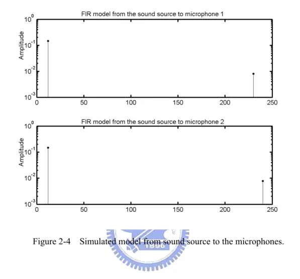
Figure 2-4 Simulated model from sound source to the microphones. ...24

Figure 2-5 The histograms of IPDs and ILDs of the first sound source.. ...25

Figure 2-6 The histogram of IPDs and ILDs of the second sound source...26

Figure 2-7 Relation between the value of a₁ and the IPD...29

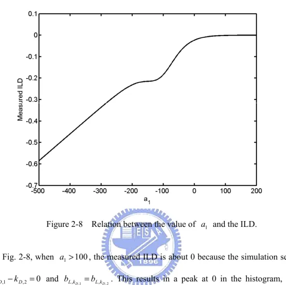
Figure 2-8 Relation between the value of a₁ and the ILD...31

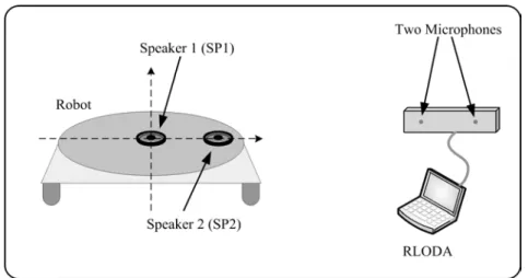
Figure 3-1 Speaker and microphone configuration of the proposed system. ...44

Figure 3-2 Overall system architecture...45

Figure 3-3 Flowchart of the proposed system...46

Figure 3-4 Relations between β and the sound pattern...48

Figure 3-5 Simulation of generated sound pattern...49

Figure 4-1 The layout of the experimental environment. ...59

Figure 4-2 The dummy head adopted in the experiment. ...60

Figure 4-3 The experimental platform and the proposed RLODA...64

Figure 4-4 Experimental environment. ...66

Figure 4-5 The waveform and spectrogram of barking signal...67

Figure 4-6 Location detection results alone X and Y axes. ...68

Figure 4-7 The average of the measured a posteriori location probabilities...71

List of Tables

Table 4-1 Average correct rates of azimuth localization at each distance ...61 Table 4-2 Average correct rates of distance localization at each azimuth ...62 Table 4-3 Average correct rates of elevation localization at each azimuth...63 Table 4-4 Average SNRs of all trajectories and the average SNRs of each trajectory

pair (dB)...67 Table 4-5 Average correct rates of location detection results (%) ...69 Table 4-6 Average correct rates of orientation detection results (%)...70

Chapter 1

Introduction

1.1 Sound Source Localization Using Binaural Information

The task of localizing a sound source using multiple microphones has been developed for years [1]. Among various kinds of techniques, methods that are based on the auditory system of humans or other animals using two microphones are one of the most popular approaches in this research field.

Sound perceived by humans is influenced by the torso, pinna, shape of human head, and acoustic environment. To identify how the human body affects perceived sound waveforms, head-related transfer function (HRTF), or head-related impulse response (HRIR) were proposed [2 - 4]. Generally, HRIR is a measure of impulse response from the sound source to eardrums in an anechoic room [5]—HRTF is considered the Fourier transform of HRIR [6]. Since HRTF varies with the sound source location, many localization cues were discussed based on HRTF. For example, the interaural level differences (ILDs) and the interaural time differences (ITDs) are utilized as the major cues for localizing a sound source, especially for azimuth

1.1.1 Azimuth Localization Using Binaural Localization Cues

Brungart et al. concluded that ILDs play an important role in localizing sound sources near the head [8]. The ITD, or interaural phase difference (IPD), which is the frequency domain representation of ITD, can be estimated by cross-correlation functions [9] or generalized cross-correlation (GCC) methods [10, 11]. Although IPDs and ILDs have been studied for a long time, they have limitations. Based on an assumption that head and ears are symmetrical, the sound source presented at a median plane should produce no interaural difference. Therefore, interaural difference cues are insufficient for localizing the elevation of a sound source in the medium plane. Moreover, any sound source falls on a “cone of confusion,” as Woodworth called it [12], may lead to constant IPDs or ILDs.

1.1.2 Elevation Localization Using Binaural Localization Cues

Cues of spectral modification are very important for elevation localization and front-back discrimination [13]. As the sound is filtered by the pinna before reaching the eardrum, “pinna notch” was investigated [14]. The influence of head diffraction and torso reflection was also examined [15]. Therefore, the elevation of a sound source can be estimated by comparing the incoming spectrum with the stored HRTF [16, 17]. These elevation estimation methods typically assume a flat sound spectrum or one that is known in advance. In practice, natural sounds are highly nonstationary and localization systems have no a priori knowledge of the spectrum shape of the nature sound [16]. Although most research results showed that spectral modification cues are significant for elevation localization, it remains unclear how the human auditory system localizes the elevation of nonstationary sound [16].

1.1.3 Distance Localization Using Binaural Localization Cues

Another significant localization ability of the human auditory system is distance localization. Research works indicated that many possible cues exist for distance localization (e.g., overall sound source intensity and energy ratio of direct to reverberant sound [7] [18]). However, overall sound source intensity can only be employed for relative distance localization and the energy ratio of direct to reverberant sound is strongly influenced by the reflections within an application environment [7]. Therefore, sound source localization in three-dimensional environments using binaural information remains an open research topic.

1.2 An Overview of Microphone-Array-Based Direction of

Arrival Estimation

Besides HRTF based approaches, methods based on multiple microphones or microphone array are proposed. Figure 1-1 shows the physical layout of a uniform linear microphone array.

where x denotes the sound source, y₁

( )

n _Ly_M

( )

n denotes the signal received by M microphones, y_ref

( )

n denotes the signal received by the reference microphone,

A

L is the size of the microphone array and d , _x θ_x are the distance and azimuth from the sound source to the reference microphone. Based on the relation between

A

L and d , the received signals can be regard as plane waves (far-field) or spherical _x waves (near-field). The definition of far-field and near field can be found in [19].

Generally, existing microphone-array-based sound source localization algorithms may be divided into three categories: steer-beamformer-based algorithms, eigen-structure-based direction of arrival (DOA) estimation algorithms, and time-delay of arrival (TDOA) based algorithms.

1.2.1 Steer-Beamformer-Based Algorithms

Steer-beamformer-based sound source localization algorithms [20 - 22] utilize beamformer algorithms to form beams for spatial filtering and steer the formed beam to the interested directions to obtain the spatial response. The power of the spatial response is then computed and the most possible sound source direction is decided by finding the direction with maximum power. The performance of steer-beamformer-based algorithm depends mainly on the resolution of the beamformer and the steer-beam algorithm adopted. Therefore, the performance of steer-beamformer-based sound source localization algorithms is limited by the resolution of beamformer. Raising the resolution of beamformer and increasing the steered beam direction result in higher computational load.

1.2.2Eigen-Structure-Based DOA Estimation Algorithms

The eigen-structure-based DOA estimation algorithms [23 - 34] are proposed for high-resolution multiple sound source localization. This kind of sound source localization algorithms derive the data correlation matrix from the signals obtained from the microphone array and compute the eigenvectors. The eigenvectors are separated into two subspaces, signal subspace and noise subspace, according to the importance of eigenvalue. Based on the theory in [24], the array manifold vector (or the steering vector), a

( )

θ , corresponds to the sound source localization and is orthogonal to the noise subspace. Consequently, the projection of a

( )

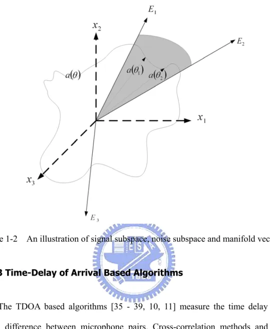
θ to the noise subspace must be zero theoretically when θ consists the direction of sound source.

Figure 1-2 is a three-dimensional example of the relation between signal subspace, noise subspace and manifold vectors, where E₁ and E₂ are the eigenvectors that span signal subspace, and E is the eigenvector that span noise ₃ subspace. Therefore, the manifold vector a

( )

θ is orthogonal to E when ₃

2 1or θ

θ

θ = . According to this relation, the location of sound sources can be estimated. The drawbacks of eigen-structure-based DOA estimation algorithms are the ability of dealing with reverberant signal and the requirement of eigenvalue decomposition. When the environment is reverberant, the eigen-structure of the data correlation matrix would break the assumption above and result in an un-robust estimation result. On the other hand, the requirement of eigenvalue decomposition makes eigen-structure-based DOA estimation algorithms need more processing power.

Figure 1-2 An illustration of signal subspace, noise subspace and manifold vectors.

1.2.3 Time-Delay of Arrival Based Algorithms

The TDOA based algorithms [35 - 39, 10, 11] measure the time delay using phase difference between microphone pairs. Cross-correlation methods and GCC methods discussed in 1.1.1 can also be classified in this category. The time delay is then combined with the geometric relation between sound source and microphones to estimate the most possible sound source location. Basically, TODA based algorithms require lower computation power then methods in the other two categories. However, TODA based algorithms are sensitive to the weights of processed frequencies. Works on how to select a set of optimal weight are proposed and discussed in this research field.

1.3 Known Problems in Sound Source Localization

Early experimental results for HRTF were principally obtained in anechoic rooms using maximum-length sequence (MLS) method [40]. Since this approach is based on stationary sound sources in anechoic rooms, conventional studies of HRTF mainly concentrated on the steady-state response from a sound source to the eardrums caused by human body. Only a few studies addressed the issue of localizing a sound source in a reverberant room [14] [41]. In a real enclosure, the relation between a sound source and microphones is very complicated and is almost impossible to characterize with a finite-length data and short-term analysis method such as short-term Fourier transform (STFT). According to the investigation of room acoustics [42], the number of eigen-frequencies with an upper limit of f_s/2Hz can be obtained by the following equation:

3 2 3 4 ⎟ ⎠ ⎞ ⎜ ⎝ ⎛ Ψ = ν π fs L (1-1)

where f denotes the sampling frequency, _s ν represents the sound velocity ( ν ≈340m/s ) and Ψ is the geometrical volume. This equation indicates that the number of poles is too high when the frequency is high, and that the transient response occurs in almost any processing duration when the input signal is a nonstationary sound. For example, the number of poles is about 96435 when the sampling frequency is 8000 Hz and the volume is 14.1385 m3. Hence, the nonstationary characteristic of nature sound source makes the IPDs and ILDs between the signals received by two microphones from a fixed sound source vary among data

In practice, reverberant sounds can significantly influence the localization cues. Gustafsson et al. analyzed how reverberation can distort time-delay estimation [43]. Shinn-Cunningham et al. showed that HRTFs are altered by reverberant sound in a classroom [44, 45] and the reverberation can cause temporal fluctuation in short-term IPDs and ILDs [44]. These studies suggest that the performance of general methods of sound source localization based on a set of HRTFs measured in anechoic rooms with stationary sound sources can be limited because of the nonstationary property of natural sound, reverberation, and short-term frequency analysis. Based on the precedence effect, some sound source localization methods excluded reverberant sound by detecting sound source onset [46]. However, as mentioned above, reverberation actually helps listeners judge the distance of sound source. Excluding reverberant sound can restrict the ability for distance localization.

Besides reverberation and nonstationarity of sound source, there are still other non-ideal issues such as the non-line-of sight condition and microphone mismatch problem. When only two microphones are used, the methods mentioned above estimate mainly the difference between microphones. It means that the methods cannot distinguish between different sound sources, which are aligned relative to the array under far-field condition. Furthermore, barriers may exist between microphones and sound source (so-called the non-line-of sight condition) in real applications. Under these circumstances, these methods estimate only the directions of reflection or diffraction, and cannot determine the real source direction. In practice, microphone mismatch is also an important issue, since the methods above assume that microphones are mutually matched. Pre-matched microphones are relatively expensive and the microphone calibration procedure is not always reliable because the characteristic of microphone changes with sound direction and is hard to measure

precisely.

1.4 Contribution of this Dissertation

This work focuses on localizing sound source in complex indoor environment. Unlike traditional works that try to eliminate the influence of the temporal fluctuation caused by reverberations, this work attempts to model these fluctuations using statistical models for sound source localization.

In the first part of this work, the relation between the nonstationarity of sound source and the distribution patterns of IPDs and ILDs when short-term frequency analysis is utilized for analysis is discussed. The level fluctuation of nonstationary sound source is modeled by the exponential of polynomials based on the concept of moving pole model. Accordingly, the sufficient condition for utilizing the distribution patterns of IPDs and ILDs to detect the location of nonstationary sound source is suggested and the phenomena of multiple peaks in the distribution patterns can also be explained. Furthermore, a Gaussian mixture based model, called Gaussian-mixture binaural room distribution model (GMBRDM) is proposed to model the distribution patterns of IPDs and ILDs for nonstationary sound source localization.

In the second part, the related research is applied to robot’s location and orientation detection. An indoor sound field feature matching method is proposed and is applied to detect a mobile robot’s location and orientation. The sound field feature, captured from a sound source to a pair of microphones, contains the dynamic of the propagation path. Because of the complexity of indoor environment, the features from

models (GMMs) [53] are utilized in this work to characterize the phase difference and magnitude ratio distributions between the microphone pair in consecutive data frames. The application provides an alternative thinking compared with traditional methods such as DOA estimation using propagation delay. They usually suffer from reverberation, non-line-of-sight and microphone mismatch problems.

1.5 Organization of this Dissertation

This dissertation is organized as follows. This chapter provides a brief introduction to the general sound source localization algorithms, including methods which follow the auditory system of human and methods based on microphone array. Moreover, this chapter also discusses the main contribution and the organization of this dissertation. In the next chapter, the binaural room distribution pattern and related GMBRDM are introduced. In Chapter 3, sound based robot’s location and orientation detection system is proposed and discussed. The related experiments are shown in Chapter 4. Chapter 5 gives some conclusion remarks and avenues for future research.

Chapter 2

Nonstationary Sound Source

Localization Using Binaural Room

Distribution Pattern

2.1 Introduction

As discussed in the first chapter, localizing a nonstationary sound source in a reverberant environment can face temporal fluctuation of interaural cues. Recent research results for sound source localization revealed the importance of temporal fluctuation phenomenon of IPDs and ILDs. Rather than eliminate the influence of these fluctuations, these studies attempted to describe these fluctuations using statistical models for sound source localization [56]. The work in [48] investigated localization cues of IPDs and ILDs exhibiting temporal fluctuation phenomena when sound sources are nonstationary and short-term frequency analysis, such as short-term Fourier transform (STFT), is utilized. In [48], distribution patterns of IPDs and ILDs were calculated from the superposition of sound sources recorded in an anechoic

patterns were applied to estimate the azimuth and elevation of a sound source using Bayesian maximum a posteriori estimation. The experiments demonstrated good results in both quiet and noisy conditions. Further, Smaragdis and Boufounos [49] also used the Gaussian model to model the empirical features in a reverberant room. In their work, the fluctuation of relative magnitude and phase of the cross spectra is modeled for sound source localization and the wrapping effect is solved using the proposed wrapped Gaussian model.

This study attempts to probe further the cause of IPD and ILD distribution patterns when a sound source is nonstationary and STFT is utilized. To simplify the description, distribution patterns of IPDs and ILDs are called binaural room distribution patterns (BRDPs) in the remainder of this work. The idea of moving pole model is employed to model the nonstationary sound sources; consequently, the level fluctuation is modeled as an exponent of polynomial. Based on this model, it can be shown that BRDPs depend on the content of the nonstationary source signals. The dependency is analyzed to explain the phenomenon of multiple peaks in the BRDPs.

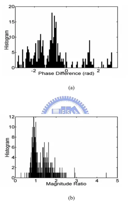
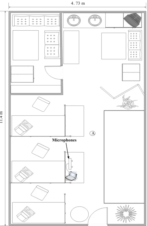
In real environment, more than one peak can exist in the measured BRDPs. For example, Fig. 2-1 illustrates the IPDs and ILDs measured at the location marked “A” in Fig. 2-2.

(a)

(b)

Figure 2-1 The histograms of IPDs and ILDs measured at location the marked “A”. (a) The histogram of IPDs at the location marked “A”. (b) The histogram of ILDs at the location marked “A”.

As shown in Fig. 2-1, the IPD and ILD contain multiple peaks. This phenomenon can be explained with the proposed model.

Since the BRDPs can contain multiple peaks, a modeling method that deals with complicated distribution patterns is needed. Although the work in [48] utilized normalized histograms to model distribution patterns, the memory requirement is considerable when histogram resolution is high. Therefore, this work adopts GMMs to model BRDPs and proposes a GMBRDM to parameterize them. Because the proposed GMBRDM is a linear combination of the phase difference GMM and the magnitude ratio GMM, a method is proposed to obtain the optimal weights of the linear combination to enhance the localization ability. Additionally, because BRDPs contain information on direct paths and reflections, localizing a sound source in the azimuth, elevation and distance using the proposed GMBRDM is possible.

The remainder of this chapter is organized as follows. The next section discusses how the nonstationary sound source can influence the IPD and ILD. A simulation of a simplified environment is performed to verify the discussion in Section 2.3. Section 2.4 presents the formulation of the proposed GMBRDM. The summary is given in Section 2.5.

2.2 The Relation between the Nonstationary Sound Source

and the BRDP

2.2.1 IPDs and ILDs of Stationary Sound Source

A linear time-invariant (LTI) room acoustic channel is represented by a K tapped finite impulse response (FIR) model

( )

∑

−

(

)

= − = 1 0 K k k k n b n h δ as,

( )

_∑

−

(

)

= − = 1 0 K k k k n x b n y (2-1)

where x

( )

n denotes sound signal emitted into the channel, y

( )

n denotes the signal received by the ear, and b is the coefficients of the FIR model for the room impulse _k response (RIR) from sound source to an ear. Without lost of generality, the stationary input signal is assumed to be a complex exponential signal with frequency ωˆ and constant level A :

( )

_{n Ae}j n x ₌ ωˆ _(2-2) where N kˆ 2 ˆ π

ω = , which is the sampled frequency of an N-point STFT. For such input, the corresponding output is

( )

(

)

(

)

j n K k k j k K k k n j k K k k Ae e b Ae b k n x b n y ω ω ω ˆ 1 0 ˆ 1 0 ) ( ˆ 1 0

∑

∑

∑

− = − − = − − = = = − = (2-3)

Take the N-point STFT at frequency ωˆ:

( )

∑

∑ ∑

− = − − = − − = − = ⎟ ⎠ ⎞ ⎜ ⎝ ⎛ = 1 0 ˆ 1 0 ˆ ˆ 1 0 ˆ ˆ K k k j k N n n j n j K k k j k e b NA e Ae e b Y ω ω ω ω ω (2-4)

By denoting y_L

( )

n and y_R

( )

n as the signals received by left and right ears, respectively, and Y_L(ωˆ) and Y_R(ωˆ) are the STFT of y_L

( )

n and y_R

( )

n , the IPD,

) ˆ (ω

P , and ILD, M(ωˆ), between Y_L(ωˆ) and Y_R(ωˆ) are

⎟ ⎟ ⎟ ⎟ ⎠ ⎞ ⎜ ⎜ ⎜ ⎜ ⎝ ⎛ ∠ =

∑

∑

− = − − = − 1 0 ˆ , 1 0 ˆ , ) ˆ ( _K k k j k R K k k j k L e b e b P ω ω ω and

∑

∑

− = − − = − = ₁ 0 ˆ , 1 0 ˆ , ln ) ˆ ( _K k k j k R K k k j k L e b e b M ω ω ω (2-5)

where b_L,k and b_R,k are the coefficients of FIR channel models, h_L and h_R, from the sound source to the left ear and the right ear,

∑

−

(

)

= − = 1 0 , K k k L L b n k h δ ,

(

)

∑

− = − = 1 0 , K k k R R b n k

h δ and ∠

( )

⋅ denotes the phase value. Note that the operation of nature logarithm is taken for computing the magnitude ratio. As shown in (2-5), the IPD and ILD between Y_L(ωˆ) and Y_R(ωˆ) depend only on the frequency responses of the channels and the measured frequency, as discussed in related research.

2.2.2 IPDs and ILDs of Nonstationary Sound Source

Although the nonstationarity of a sound source can be tested in many different domains [50], this work only considers time domain variation. To model time domain variation of a sound source, the level of the complex exponential signal in (2-2) is assumed as time varying:

( )

j j n ne e A n

x ₌ φ ωˆ _(2-6)

where A is a time-varying sound level. Accordingly, the output _n y

( )

n can be formulated as:

( )

(

)

∑

∑

∑

− = − − − = − − − = = = − = 1 0 ˆ ˆ 1 0 ) ( ˆ 1 0 K k n j j k j k k n K k k n j j k n k K k k e e e b A e e A b k n x b n y ω φ ω ω φ _(2-7)

Take the STFT at frequency ωˆ:

( )

(

)

∑∑

∑∑

∑

− = − = − − + − = + − − = + − − + − = + − = = + = 1 0 1 0 ˆ 1 0 ) ( ˆ 1 0 ) ( ˆ ˆ 1 0 ) ( ˆ ˆ , N K k j k j k k n N n j K k n j j k j k k n N n j e e b A e e e e b A e n y n Y τ φ ω τ τ τ ω τ ω φ ω τ τ τ ω τ ω (2-8)

∑∑

∑∑

− = − = − − + − = − = − − + = ₁ 0 1 0 ˆ , 1 0 1 0 ˆ , ) ˆ , ( ) ˆ , ( N K k k j k R k n N K k k j k L k n R L e b A e b A n Y n Y τ ω τ τ ω τ ω ω _(2-9)

and )P(n,ωˆ and M(n,ωˆ) between Y_L(n,ωˆ) and Y_R(n,ωˆ) are

⎟ ⎟ ⎟ ⎟ ⎠ ⎞ ⎜ ⎜ ⎜ ⎜ ⎝ ⎛ ∠ =

∑∑

∑∑

− = − = − − + − = − = − − + 1 0 1 0 ˆ , 1 0 1 0 ˆ , ) ˆ , ( _{N K} k k j k R k n N K k k j k L k n e b A e b A n P τ ω τ τ ω τ ω , and

∑∑

∑∑

− = − = − − + − = − = − − + = ₁ 0 1 0 ˆ , 1 0 1 0 ˆ , ln ) ˆ , ( _{N K} k k j k R k n N K k k j k L k n e b A e b A n M τ ω τ τ ω τ ω (2-10)

As shown in (2-10), the phase difference and magnitude ratio become content dependent when STFT is utilized and A is nonstationary. _n

2.2.3 Modeling the Nonstationary Sound Source Using Moving Pole Model

To analyze how nonstationarity of a sound source influences the IPD and ILD, a parameterized model for nonstationary sound is needed. Based on the discussion in [51] and [52], a nonstationary sound source in an analysis window can be expressed as a sum of moving pole models. In this work, the idea in [52] that approximate A _n as an exponent of polynomial is utilized. In [52],

∑ = = ⎟⎟⎠ ⎞ ⎜⎜ ⎝ ⎛ a N t t s t f n a n e A 0 (2-11)

where N is the degree of the polynomial, _a a is the coefficient of the polynomial _t and f denotes the sampling frequency. To simplify the analysis, we omit the terms _s of t≥2, as in [30]; hence, A is modeled as: _n

1 0 a f n a n e s A = + (2-12)

Substituting (2-12) into (2-8), Y_L(n,ωˆ) can be rewritten as:

φ ω φ ω φ ω φ ω ω j K j K L a f K N n a a f K n a a f K n a a f K n a j j L a f N n a a f n a a f n a a f n a j j L a f N n a a f n a a f n a a f n a j j L a f N n a a f n a a f n a a f n a L e e b e e e e e e b e e e e e e b e e e e e e b e e e e n Y s s s s s s s s s s s s s s s s ) 1 ( ˆ 1 , ) ( ) 3 ( ) 2 ( ) 1 ( 2 ˆ 2 , 3 1 2 1 ˆ 1 , 2 1 1 0 ˆ 0 , 1 2 1 1 0 1 0 1 0 1 0 1 0 1 0 1 0 1 0 1 0 1 0 1 0 1 0 1 0 1 0 1 0 1 0 ) ˆ , ( − − − ⎟⎟ ⎠ ⎞ ⎜⎜ ⎝ ⎛ + − + ⎟⎟ ⎠ ⎞ ⎜⎜ ⎝ ⎛ − − + ⎟⎟ ⎠ ⎞ ⎜⎜ ⎝ ⎛ − − + ⎟⎟ ⎠ ⎞ ⎜⎜ ⎝ ⎛ − − + − ⎟⎟ ⎠ ⎞ ⎜⎜ ⎝ ⎛ + − + ⎟⎟ ⎠ ⎞ ⎜⎜ ⎝ ⎛ + ⎟⎟ ⎠ ⎞ ⎜⎜ ⎝ ⎛ − + ⎟⎟ ⎠ ⎞ ⎜⎜ ⎝ ⎛ − + − ⎟⎟ ⎠ ⎞ ⎜⎜ ⎝ ⎛ + − + ⎟⎟ ⎠ ⎞ ⎜⎜ ⎝ ⎛ + + ⎟⎟ ⎠ ⎞ ⎜⎜ ⎝ ⎛ + ⎟⎟ ⎠ ⎞ ⎜⎜ ⎝ ⎛ − + − ⎟⎟ ⎠ ⎞ ⎜⎜ ⎝ ⎛ + − + ⎟⎟ ⎠ ⎞ ⎜⎜ ⎝ ⎛ + + ⎟⎟ ⎠ ⎞ ⎜⎜ ⎝ ⎛ + + ⎟⎟ ⎠ ⎞ ⎜⎜ ⎝ ⎛ + ⎥ ⎥ ⎦ ⎤ ⎢ ⎢ ⎣ ⎡ + + + + + ⎥ ⎥ ⎦ ⎤ ⎢ ⎢ ⎣ ⎡ + + + + + ⎥ ⎥ ⎦ ⎤ ⎢ ⎢ ⎣ ⎡ + + + + + ⎥ ⎥ ⎦ ⎤ ⎢ ⎢ ⎣ ⎡ + + + + = L M L L L ` (2-13)

This equation can be rearranged as: ( ) φ ω φ ω φ ω φ ω φ ω ω j K k k j k L k f a f a f a N a f n a j K j K L a f N a f a f a f n a f a K j j L a f N a f a f a f n a f a j j L a f N a f a f a f n a f a j j L a f N a f a f a f n a L e e b e e e e e e b e e e e e e e b e e e e e e e b e e e e e e e b e e e e n Y s s s s s s s s s s s s s s s s s s s s s s s ⎟ ⎟ ⎠ ⎞ ⎜ ⎜ ⎝ ⎛ − − = ⎥ ⎥ ⎦ ⎤ ⎢ ⎢ ⎣ ⎡ + + + + + + ⎥ ⎥ ⎦ ⎤ ⎢ ⎢ ⎣ ⎡ + + + + + + ⎥ ⎥ ⎦ ⎤ ⎢ ⎢ ⎣ ⎡ + + + + + + ⎥ ⎥ ⎦ ⎤ ⎢ ⎢ ⎣ ⎡ + + + + + =

∑

− = − − + − − − − + − − − − + − − − + − − − + 1 0 ˆ , ) 1 ( ˆ 1 , ) 1 ( 2 1 1 2 ˆ 2 , ) 1 ( 2 1 2 1 ˆ 1 , ) 1 ( 2 1 0 ˆ 0 , ) 1 ( 2 1 1 1 1 1 0 1 1 1 1 0 1 1 1 1 1 0 1 1 1 1 1 0 1 1 1 1 1 0 1 1 1 1 1 1 ) ˆ , ( L M L L L (2-14)

Through the same procedure, we have

φ ω ω K j k k j k R k f a f a f a N a f n a R e b e e e e e n Y s s s s ⎟ ⎟ ⎠ ⎞ ⎜ ⎜ ⎝ ⎛ − − =

∑

− = − − + 1 0 ˆ , 1 1 1 1 0 1 1 ) ˆ , ( (2-15)

and the ratio between Y_L(n,ωˆ) and Y_R(n,ωˆ) becomes:

∑

∑

− = − − − = − − = 1 0 ˆ , 1 0 ˆ , 1 1 ) ˆ , ( ) ˆ , ( K k k j k R k f a K k k j k L k f a R L e b e e b e n Y n Y s s ω ω ω ω _(2-16)

Consequently, the IPD and ILD are ⎟ ⎟ ⎟ ⎟ ⎟ ⎠ ⎞ ⎜ ⎜ ⎜ ⎜ ⎜ ⎝ ⎛ ∠ =

∑

∑

− = − − − = − − 1 0 ˆ , 1 0 ˆ , 1 1 ) ˆ , ( K k k j k R k f a K k k j k L k f a e b e e b e n P s s ω ω ω and

∑

∑

− = − − − = − − = 1 0 ˆ , 1 0 ˆ , 1 1 ln ) ˆ , ( K k k j k R k f a K k k j k L k f a e b e e b e n M s s ω ω ω (2-17)

By observing (2-17), this study finds that the IPD and ILD values depend on the coefficient of the FIR models and the value of a₁, which is the slope of the nature logarithm of A . _n

2.3 Simulation Verification and Discussion of Proposed

Model

2.3.1 Content Dependency of BRDPs Obtained from Nonstationary Sound Source

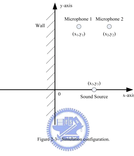
To verify the proposed analysis, a simplified simulation environment (Fig. 2-3) is assumed (Although the simplified environment is utilized as an example here, the following discussion of the relationship between BRDPs and nonstationary sound sources can be applied to general cases).

Figure 2-3 Simulation configuration.

As depicted in Fig. 2-3, the only cause of reflection is the only cause of reflection is the infinite wall located at x=0. The two microphones are located at

(

x₁,y₁,z₁

) (

= 4.8m,0.5m,0m

)

and

(

x₂,y₂,z₂

) (

= 5.2m,0.5m,0m

)

and the sound source is located at

(

x₃,y₃,z₃

) (

= 5m,0m,0m

)

. The models from the sound source to the microphones are simulated by the image method introduced in [47] with sound speed c=340m s and sampling rate fs =8000Hz. The wall is assumed to be rigid. The simulated model is depicted in Fig. 2-4.

Figure 2-4 Simulated model from sound source to the microphones.

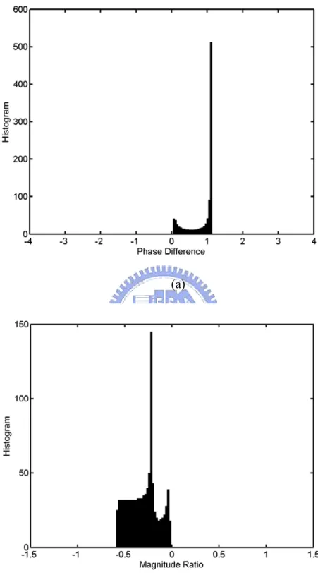
Two different sources are input into the simulation model to show the content dependency of IPD and ILD histograms. For the first source, the value of a₁ in the measured frames is uniformly distributed between

[

−500,0

]

. The IPDs and ILDs at a frequency of 140.625 Hz are computed 1000 times. Fig. 2-5 presents the histograms, which can represent the probability distribution, of IPDs and ILDs. The second source is similar to the first, except the value of a₁ is uniformly distributed between

(a)

(b)

Figure 2-5 The histograms of IPDs and ILDs of the first sound source. (a) The histogram of IPDs of the first sound source. (b) The histogram of ILDs of the first

(a)

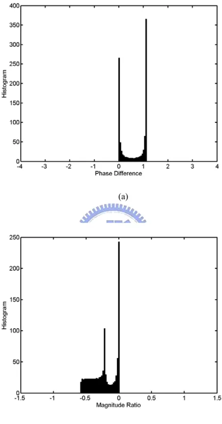
(b)

Figure 2-6 The histograms of IPDs and ILDs of the second sound source. (a) The histogram of IPDs of the second sound source. (b) The histogram of ILDs of the second sound source.

The simulation results in Figs. 2-5 and 2-6 demonstrate that when the sound sources are nonstationary, the IPD and ILD histograms depend on the content of the source signal. Therefore, conditions of the nonstationary sound source must be designed such that the BRDPs can be utilized for localization. In view of the aforementioned discussion, the sufficient condition is that the distribution of a₁ of the sound source must be stationary to make the sound source applicable for localization. Care must be exercised when using IPDs and ILDs obtained from nonstationary sound sources for sound source localization to avoid performance degradation.

2.3.2 The Formation of Peaks in the Distribution Patterns of IPDs

As shown by the simulation in Section 2.3.1, the distribution patterns of IPDs exhibit multiple peaks. This phenomenon also appears in the empirical results in real environment. The derivation result of (2-17) can be adopted to explain this phenomenon.

According to (2-17), there are several possible reasons to form peaks in the distribution patterns of IPDs. First, if a₁ of a sound source is concentrated at a certain value, a peak in the histogram will result. An obvious example is a stationary sound source. For a stationary sound source, a₁ =0 for all measured frames, which makes IPD a fixed value, results in a peak in the distribution pattern.

Secondly, the term f k a

s

e

1

−

in (2-17) decreases as k increases when a₁ is positive. This means the weights of the reflection part in the channel model is reduced and the influence of the direct path are increased. Hence, when a₁ exceeds a certain

⎟⎟ ⎠ ⎞ ⎜⎜ ⎝ ⎛ ∠ = ⎟ ⎟ ⎟ ⎟ ⎠ ⎞ ⎜ ⎜ ⎜ ⎜ ⎝ ⎛ ∠ ≈ − − − − − − 2 , 1 , 2 , 2 , 2 , 1 1 , 1 , 1 , 1 ˆ ˆ ˆ , ˆ , ) ˆ , ( D D D D D s D D D s k j k j k j k R k f a k j k L k f a e e e b e e b e n P ω ω ω ω ω (2-18)

where k and _D,1 k_D,2 are propagation delay of the direct path from the sound source to microphones. Based on (2-18), the phase difference between direct paths from a sound source to microphones is emphasized and can dominate the measured IPDs. Since the IPDs are approximately the same for all a₁ exceed a certain level, a peak can be formed in the distribution pattern. This derivation explains why some previous research results of IPD-based time delay estimation suggested utilizing speech source onset to improve the accuracy [24]. On the contrary, when a₁ is negative, the value of f k a s e 1 −

increases with k. In this case, the influence of the direct path is suppressed and the reflections can dominate the measured IPDs.

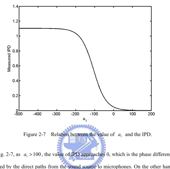
The second simulation in Section 2.3.1 is utilized to interpret the relationship between a₁ and the IPD (Fig. 2-7).

Figure 2-7 Relation between the value of a₁ and the IPD.

In Fig. 2-7, as a₁>100, the value of IPD approaches 0, which is the phase difference caused by the direct paths from the sound source to microphones. On the other hand, when a₁ <−300, the value converges to 1.1, representing the phase difference influenced by wall reflection. It is then easy to understand why there are two peaks at 0 and 1.1 in Fig. 2-6 (a). Generally, reflections appear later in the propagation model than direct paths, meaning that a negative value of a₁ is required to emphasize the effect of reflections. Consequently, the more the wall or boundary absorbs the energy of sound source, the smaller value of negative a₁ is required to emphasize the effect of reflections.

2.3.3 The Formation of Peaks in the Distribution Patterns of ILDs

Similar to the discussion of IPDs, the a₁ of a sound source is concentrated at a certain value, results in a peak in the ILD distribution pattern. However, ILDs behave quite different than IPDs when a₁ is either large or small. When a₁ is larger than a certain level, M(n,ωˆ) can be approximated by

2 , 1 , 2 , 2 , 1 1 , 1 , 1 2 , 2 , 2 , 1 1 , 1 , 1 , 1 , , 2 , 1 , 1 , , ˆ , ˆ , ln ) ( ln ln ) ˆ , ( D D D D s D D s D D D s D D D s k R k L s D D k R k f a k L k f a k j k R k f a k j k L k f a b b f k k a b e b e e b e e b e n M + − − = = ≈ − − − − − − ω ω ω (2-19)

Therefore, the relationship between ILDs and a₁ is approximately linear (with a slope of s D D f k k ) ( _,1− _,2 −

) when a₁ is larger than a certain level. Hence, if the slope is 0 (meaning k_D,1=k_D,2), it will cause a peak in the ILD histogram. Similar to IPDs, when a₁ is smaller than a certain level, the influence of the direct path is de-emphasized and the reflection part starts dominating the measured ILDs. The second simulation in Section 2.3.1 is again utilized as an example of the discussion above. Figure 2-8 shows the simulation results for the relationship between the value of a₁ and the ILD.

Figure 2-8 Relation between the value of a₁ and the ILD.

In Fig. 2-8, when a₁>100, the measured ILD is about 0 because the simulation sets 0 2 , 1 , − D = D k

k and b_L,kD,1 =b_L,kD,2. This results in a peak at 0 in the histogram, as shown in Fig. 2-6 (b). In addition, when a₁ <−300, the measured ILDs change linearly with the value of a₁, resulting in a flat area in Fig. 2-6 (b).

2.3.4 Localization of Nonstationary Sound Source Using BRDPs

As mentioned in Chapter 1, detecting the location of sound sources presented at median plane or on a “cone of confusion” is difficult when only IPDs and ILDs of direct paths are utilized. However, sound sources at different locations can propagate through different reflections and with the property of nonstationary sound source discussed above, the nonstationary sound can result in distinguishable distribution

azimuth, elevation, and distance using BRDPs.

2.4 GMBRDM for Nonstationary Sound Source Localization

As discussed in Section 2.3.1, if the environment and head position are unchanged and the distribution of a₁ of the sound source is stationary, using BRDPs for sound source localization is possible. Sections 2.3.2 and 2.3.3 also show that BRDPs can be non-Gaussian and contain multiple peaks. Consequently, modeling these distribution patterns as a simple distribution pattern (such as a single Gaussian distribution) can eliminate important details. Utilizing a high-resolution normalized histogram to model the distribution pattern requires considerable computational of memory. In this work, GMMs are employed to model BRDPs (called the GMBRDM) to reduce the memory requirement through parameterization.

2.4.1 The Training Procedure of the Proposed GMBRDM

Let P_x

(

n_f,ω_b

)

and M_x

(

n_f,ω_b

)

denote the phase difference and magnitude ratio obtained at frame n respectively for constructing GMM at frequency _f ω_b,

{

B

}

b∈ 1,..., , which means B frequencies are utilized to construct the model. The

phase difference and magnitude ratio GMMs are defined as the weighted sum of N₁ and N₂ mixtures of Gaussian component densities:

( )

(

)

i

(

x

( )

f

)

N i i P P f x n g n G P

∑

P = = 1 1 , |λ ρ (2-20)

( )

(

)

i

(

x

( )

f

)

N i i M M f x n g n G M

∑

M = = 2 1 , |λ ρ (2-21)

whereP_x

( )

n_f =

[

P_x

(

n_f,ω₁

)

_L P_x

(

n_f,ω_B

)

]

T,

( )

[

(

)

(

)

]

T B f x f x f x n = M n ,ω1 L M n ,ω

M . ρ_P,i and ρ_{M ,i} are the weights of ith mixture, and g_i

(

P_x

( )

n_f

)

and g_i

(

M_x

( )

n_f

)

are the Gaussian density functions. Notably, the mixture weights must satisfy the constraints:

1 1 1 , =

∑

= N i i P ρ and 2 1 1 , =

∑

= N i i M ρ (2-22)

The terms λ and _P λ represent the parameters of _M N and ₁ N₂ component densities.

{

P P P

}

P μ Σ λ = ρ , , and λ_M =

{

ρ_M,μ_M,Σ_M

}

(2-23) where

[

P,1 P,N1

]

P = ρ L ρ

ρ denotes the phase difference mixture weight vector with dimensions 1 N× ₁.

[

M,1 M,N2

]

M = ρ L ρ

ρ denotes the magnitude ratio mixture weight vector with dimensions 1 N× ₂.

[

P,1 P,N1

]

P = μ L μ

μ denotes the phase difference mean matrix with dimensions

1

N B× .

[

M,1 M,N2

]

M = μ L μ

[

P,1 P,N1

]

P Σ Σ

Σ = _L denotes the phase difference covariance matrix with dimensions B×BN₁.

[

M,1 M,N2

]

M Σ Σ

Σ = _L denotes the magnitude ratio covariance matrix with dimensions B×BN₂.

The parameters λ and _P λ in (2-23) can be estimated by the iterative EM _M

algorithm [53] which guarantees a monotonic increase in the model’s log-likelihood value. By denoting the training sequence length as N_F, the iterative procedure can be divided into the expectation step and maximum step:

Expectation step:

( )

(

)

(

( )

)

i

(

x

( )

f

)

N i Pi f x i i P P f x n g n g n i G P P

∑

P = = 1 1 , , , | λ ρ ρ (2-24)

( )

(

)

(

( )

)

i

(

x

( )

f

)

N i Mi f x i i M M f x n g n g n i G M M

∑

M = = 2 1 , , , | λ ρ ρ (2-25)

where G

(

i| P_x

( )

n_f ,λ_P

)

and G

(

i| M_x

( )

n_f ,λ_M

)

are a posteriori probabilities.

Maximization step:

(i). Estimate the mixture weights:

( )

(

)

∑

= = F f N n P f x F i P N Gi n 1 , 1 |P ,λ ρ (2-26)

( )

(

)

∑

= = F f N n x f M F i M N Gi n 1 , 1 |M ,λ ρ (2-27)

(ii). Estimate the mean vector:

( )

(

) ( )

∑

(

( )

)

∑

= = = F f F f n n x f P N n x f P x f i P, ₁Gi|P n ,λ P n ₁Gi|P n ,λ μ (2-28)

( )

(

) ( )

∑

(

( )

)

∑

= = = F f F f N n x f M N n x f M x f i M, ₁Gi|M n ,λ M n ₁Gi|M n ,λ μ (2-29)

(iii). Estimate the variances:

( )

(

(

( )

) (

)

(

( )

)

)

Pi

( )

b N n x f P N n x f P x f b b i P F f F f Gi n P n ω Gi n μ ω ω σ 2 , 1 1 2 2 , =

∑

₌ |P ,λ ,

∑

₌ |P ,λ − (2-30)

( )

(

(

( )

) (

)

(

( )

)

)

Mi

( )

b N n x f M N n x f M x f b b i M F f F f Gi n M n ω Gi n μ ω ω σ 2 , 1 1 2 2 , =

∑

₌ |M ,λ ,

∑

₌ |M ,λ − (2-31)

The EM algorithm is sensitive to the choice of initial model. A good choice of initial model results in a lower number of iterations of the EM algorithm. K-means related approaches are known to be effective in finding a suitable initial model [54]. This work utilizes an accelerated K-means algorithm proposed by Elkan [55], which can significantly reduce the computational power requirement.

GMBRDM

( )

l =α_PG

(

P_x

( )

n_f |λ_P

( )

l

)

+α_MG

(

M_x

( )

n_f |λ_M

( )

l

)

(2-32) where α_P and α_M represent the weighting factors. The values of α_P and α_M can be chosen based on the sum of the correlation values among trained locations of the phase difference GMM and magnitude ratio GMM. The GMM with higher correlation summation would be assigned a lower weight, since the ability to discriminate is considered lower under this circumstance, and vice versa. Under this principle, α_P and α_M are determined by the following formula:

( )

( )

{

}

{

( )

( )

}

⎭ ⎬ ⎫ ⎩ ⎨ ⎧ +

∑

∑

M P T M M M M M T P P P P P q q q q q q UC C UC C α α min 0 , 0 , 1 . .t _P× _M = _P> _M > s α α α α (2-33)

where q_P∈Q_P and q_M ∈Q_M are the B dimensional random vectors in the operation ranges, Q_P and Q . _M

( )

_P

[

C

(

_{P P}

( )

)

C

(

_{P P}

( )

)

C

(

_{P P}

( )

L

)

]

P λ λ λ C q = q | 1 q | 2 _L q | ,

( )

_M

[

C

(

_{M M}

( )

)

C

(

_{M M}

( )

)

C

(

_{M M}

( )

L

)

]

M λ λ λ C q = q | 1 q | 2 _L q | , and ⎥ ⎥ ⎥ ⎥ ⎥ ⎥ ⎥ ⎥ ⎦ ⎤ ⎢ ⎢ ⎢ ⎢ ⎢ ⎢ ⎢ ⎢ ⎣ ⎡ = 0 0 0 0 0 0 1 0 1 1 0 1 0 0 1 1 1 0 0 1 1 1 0 M M M M O M M L O M L L L U with dimension L×L.