Design of Two-Channel Low-Delay IIR Nonuniform-Division Filter Banks Using L1 Error Criteria

Design of two-channel low-delay

IIR

nonuniform-

division filter banks using

L1

error criteria

J.-H. Lee and W.-H. Chung

Abstract: The design of a two-channel nonuniform-division filter (NDF) bank with infinite impulse response (IIR) analysis/synthesis filters and low group delay in the sense of L1 error

criteria is considered. The problem formulation results in a nonlinear optimisation problem. Based on a variant of Karmarkar’s algorithm, the optimisation problem is solved through a frequency sampling and iterative approximation technique to find the tap coefficients and the reflection coefficients for the numerator and the denominator of the IIR analysis filters. An efficient stabilisation procedure ensures that the reflection coefficients lie in (- 1, 1). Simulation results are provided for illustration and comparison.

1 Introduction

Uniform-subband decomposition by using a quadrature mirror filter (QMF) bank is not an appropriate scheme to match the requirements for the subband coding of speech and audio signals. The most appropriate decomposition must consider the critical bands of the ear. It has been mentioned in [ 11 that these critical bands have nonuniform bandwidths and cannot be easily constructed by the conventional tree structure based on two-channel QMF banks. Hence, it is worth exploiting the design problem of two-channel nonuniform-division filter (NDF) banks.

The conditions on the analysis and synthesis filters of NDF banks, as well as methods to design them, are given in [l]. Because of the difficulty in solving the design problem with nonlinear constraints, a structure and design procedure for pseudo-QMF banks was presented in [ 2 ] . The main drawback of this method is that FIR filters with complex coefficients are required by the resulting NDF bank to reduce the aliasing distortion. Recently, one of the authors considered a structure for two-channel NDF banks and proposed design methods for optimally design- ing NDF banks based on L t and L2 error criteria in [3] and [4], respectively.

Designing an NDF bank has been widely considered in [ 1-41. However, linear-phase FIR analysis filters were employed for developing these design techniques. Although using linear-phase FIR analysis filters leads to a favourable problem formulation for design, the system delay kd of the designed NDF bank is determined by the lengths of FIR filters used and, hence, the long overall system delay of an NDF bank with linear-phase FIR analysis filters may make practical applications prohibitive. It is well known that an IIR filter requires a lower order than an FIR filter under the same stopband energy. For a

0 IEE, 2002

IEE Proceedings online no. 20020485

DOI: 10.1049/ip-vis:20020485

Paper first received 20th July 2001 and in revised form 5th April 2002 The authors are with the Department of Electrical Engineering, National Taiwan University, Taipei, 106, Taiwan, Republic of China

3 04

given passband group delay, IIR NDFs have better pass- band ripple/stopband attenuation and/or lower computa- tional complexity than FIR NDFs under the same stopband energy for the analysis and synthesis filters. Several approaches dealing with the design problem of two- channel IIR uniform-division filter banks with conven- tional filter structures have been reported in [5-71. Recently, the results of designing a two-channel low- delay IIR NDF bank using the L2 error criteria have been reported in [8].

In this paper, we consider the design of two-channel low-delay IIR NDF banks in the sense of L , error criteria. Utilising a lattice structure for the denominators of the IIR analysis filters, a design technique using a modified dual- affine scaling (MDAS) variant of Karmarkar’s algorithm [9] in conjunction with an approximation scheme is presented for efficiently solving the resulting design problem that is basically a nonlinear optimisation problem. During the design process, the proposed technique finds the tap coefficients for the numerators and the reflection coeffi- cients for the denominators of the IIR analysis filters simultaneously. It ensures the stability of the designed IIR analysis filters by incorporating an efficient stabilisa- tion procedure to make the magnitude of each reflection coefficient within - 1 and

+

1. Computer simulations show that the IIR NDF banks designed by using the proposed technique provide satisfactory performance, though the designed results are only local solutions (instead of the global optimum).

2 Two-channel low-delay NDF banks

Consider the two-channel NDF bank with the architecture given in [3] which is shown in Fig. 1. The analysis low-pass and high-pass filters are designated by Ho(z) and H l ( z ) , respectively, while the synthesis low-pass and high-pass filters are designated by FO(z) and F 1 (z), respectively. Bo(z) and B I ( z ) are two low-pass filters responsible for achieving

aliasing-free operation during the rational decimation and interpolation. It can be shown that using the modulations of multiplying exp(jnn) in the high-pass subband channel leads to the favourable result that B l ( z ) can be a low-pass

filter with real coefficients. The desired magnitude responses IEE Proc.-Vis. Image Signal Process.. Vol. 149. No. 5. October 2U02

x(nll-

a b Fig. 1 a Analysis system b Synthesis system

Two-channel NDF bunk system structure

for the analysis filters Ho(z) and H I @ ) with passband widths equal to Lon/L and L I n/L, respectively, are shown in Fig. 2;

where L = Lo

+

L1

.

a,,, and o,~ denote the related band-edge frequencies satisfying wp +os = 2nLo/L.

Assume that the associated magnitude responses are set to

Bo(w) = 1, for w E

I

B l ( o ) = 1, for w E

[o,

7

1

and

I

Further, assume that Ho(z) and H l ( z ) have zero stopband

response. As shown in [4], the input/output relationship of the NDF bank in the frequency domain is given by

where Go and GI are the resulting group delays of the upper and lower channels, respectively. WL = exp(-j2n/L). ,Sub- stituting L =Lo

+

L I , Fo(eJ") =Ho(e.iW) and Fl(e.'W) = -Hl(eJ") into (1) yields

1

+

0 wp

kLn

ws R w

L

Fig. 2 Desired magnitude responses f o r analysis filters

where:

The first term of (2) represents the response of a linear shift-invariant system T(e-'") with input X(el"), while the

other two terms represent the resulting aliasing distortion. Therefore, perfect reconstruction for a group delay kd

requires the following conditions:

PR 1: T(e'") must be equal to e-Jkd0 for all o. PR 2: The magnitude Vl(w) of Vl ( eJ" ) must be zero, i.e. V l ( w ) = 0 , for all w .

PR 3: The magnitude V 2 ( o ) of V 2 ( e J w ) must be zero, i.e. V 2 ( 0 ) = 0 , for all w .

For simplicity, assuming Go = G1, we can neglect the phase term e-JwGu in (3) and express T ( e J W ) as

Furthermore, we note from (4), (5) and L =LO

+

L1 that the aliasing distortion can be eliminated if

equals zero for wp 5 w 5 w,. Following (6) and (7), we can reformulate the conditions required for perfect reconstruc- tion as follows:

for wp 5 w 5 w, (8) Hence, the design problem of the IIR NDF banks of Fig. 1 is finding such IIR analysis filters, namely Ho(z)

305 IEE Proc-Vis. Image Signal Process., Vol. 14Y, No. 5, October 2002

and Hl(z), that the conditions listed in (8) can be approxi- mately met.

3

the L, sense

3.1 Problem formulation

Here, we consider the design of the two-channel IlR NDF as shown in Fig. 1. Let the low-pass analysis filter be an IIR filter with order Mo/No (Le. Mo zeros and NO poles) and

transfer function Ho(z) = Ao(z)/BNo(z), where the numera- tor Ao(z) is an Moth-order polynomial with tap coefficient vector a. = [aoo, uol , . . . , aoM,]', and BN,(z) is an Noth- order FIR lattice filter with reflection coefficient vector

ko = [k ol, k02,.

. .

, koN,]? The superscript T denotes the transpose operation. Similarly, let the high-pass analysis filter be an IIR filter with order M I / N 1 and transfer

function H l ( z ) = A I ( z ) / B N , ( z ) , where the numerator A l ( z ) is an M I th-order polynomial with tap coefficient vector

a l = [alo, a l l , .

.

. , alMI]T and BN,(z) is an Nlth-order FIR lattice filter with reflection coefficient vector kl = [ k l l , k l 2 , .

.

. , k l ~ , ] ? Fig. 3 shows the system structure for BNo(z) and BN,(z) which can be obtained from the following recursive formula [lo]:

Design of two-channel IIR NDF banks in

Bo@) = Q O ( Z ) 1 1

Bn(z) = Bn-l(z)

+

knz-'Qn-l(z)

Qn(Z> = knBn-I(z) + z - ' Q n - ~ ( z > (9)

Hence, the overall design task is to find the required tap and reflection coefficients {a,,, kLn} for the stable IIR filters H,(z), i = 0, 1, such that the conditions shown in (8) must be satisfied. Accordingly, we consider that the overall error function E to be minimised in the L 1 sense can be

expressed as the following weighted sum of four terms:

E = 6,

+

a61

+

PS,

+

~ 6 , (10) where 6,= - ?(e-/")Idw, 61 s2=0lHl (e'")ldw, 60= GzwylHo(e J")ldu and 6,= J21V(eJ")ldo.

Moreover, a, /3 and y represent the relative weights between the four error terms. We note from (10) that the overall error function E is a highly nonlinear function of the tap and reflection coefficients. Therefore, minimising E directly leads to a very

highly nonlinear progmmming problem in addition to the stability problem for Ho(z) and Hl(z).

3.2 Proposed design technique

Let { m i = 0, ~ 2 , . . . , m r = o p , Or+ 1 , . . . , W I + J , U I + J + I =

cos,

. . . ,

u I + j + K = TC} be a grid of equidistant frequencies distributed in the range of w = 0 to w = TC for evaluating the

magnitude response of the NDF bank and the related error

terms defined as above. Moreover, assume that the set SI contains the grid points { o1 = 0, w 2 ,

.

. . , wI= w,}, S2

contains the grid points {w1+

,,

w1+2, . . . , o l + ~ } and S3 contains the grid points { o ~ + J + I = u s , w / + J + 2 , . . . ,

o I + j + K = T C } . Then, we rewrite (1 0) as the following approximation:

A .

E = 6,

+

a i l

+

+

?it

(1 1)

l e - j k d w - T(ei"')I, A $ 1 = C O G S ,

IHl(e'"

)I,

60 =

EO

E s,lHde'"

)I

and 6, =

CIu

E w , u ~ , ucu,

Ik(eju)l. Next, we construct bT=

[ I I T , ~ + ~

PlqK rJ+21

with the ( I + J + K ) x 1 vector l I + J + K = [ l , .

. .

,l]', the

I x 1 vector p l = [a,. . . , aIT, the K x 1 vector 4 K =

[fl,

. .

. ,

PIr

and the ( J + 2 ) x 1 vector Y J + ~ = [y, . . . , y ] ?

Moreover, let el = [e:leT, lei,~eT/]T represent the error vector computed at the lth iteration, where e,,! denotes the ( I + J + K ) x 1 error vector due to Je-jkdw - ?"(e'")I computed for o E SI U S2 U S3, e:,/ the I x 1 error vector due to IH/(e'")l computed for w E S1, eo,/ the K x 1 error vector due to IH&e'")l computed for Q € S 3 and e,/ the ( J S - 2 ) x 1 error vector due to (?'(ej"')I computed for w E wp U S2 U coy, respectively, where H:(:ej"), for = 0, 1, and ?'(e'") are the frequency responses for the analysis filters and the corresponding filter bank response computed at the Ith iteration during the design process, respectively. Let AHi](ej") and A?'(e'") be the deviations for Hi[(e'")

and ?'(e'") corresponding to the filter coefficient perturba- tion performed at the lth iteration. Accordingly, ?'(eim) and

A k ' ( e i " ) are the response and the deviation related to (7). Thus, the design problem of using the L1 criteria to find the optimal coefficients can be formulated as follows: where $ a

=,CUI

E SI us2 us,

T k T

Minimise byel+,

IT, - T'+'I 5 e,,/+1

where , T~ ~ [ e - i k c i ~ ~ > e - J k @ ~

, ' . . ,

]', T I =

e - J k d W ~ + ~ + K

[ p ' ( e j ( % ) , T / ( ~ J % ) , ,

. .

, p l ( e j u i + ~ + ~ )I: H : = [H:(ej"'), H:(ejw2), . . . , ~ : ( e j ~ ' ) l T , H! = [Ki(ejW1+J+l)2 H&eju'+J+2), . . . , H ~ ( e j u ' + J + K ) ] T and V ' = [V'(eiwr), V'(ej"'+,),

. .

. , ~ ' ( e J " ' + J + l ) ] ? Moreover, the notation of lYl 5 2 denotes that the absolute value of each entry in the matrix (or vector)

Y is not greater than the value of the corresponding entry in the matrix (or vector) Z . To deal with the nonlinear

Fig.

306

3

Q ~ ( z ) = 1

Lattice structure for an Nth-order FIR luttice$lter

constraints as shown in (12), we reformulate them as follows:

where the superscript

'*'

and 'Re{x}' denote the complex conjugate and the real part of x, respectively. Assume that the perturbations performed on 'the filter coefficients are significantly small at each iteration; then the second terms due to deviations in (13) can be neglected. As a result, the constraints in (13) can be approximated by the following expressions:

Next, several useful matrices are defined as follows: U, is an (Z+J+K) x 1 vector with the mth entry given by

U,(m) = e-jkdWm - T'(e.i"rn), w, E SI U S, U S3, m = 1, 2 , .

.

. , I + J + K , diag{U,} is a diagonal matrix with the mth diagonal entry given by CJcz(m), U1 is an I x 1 vector with the mth entry given by U,(m) = -H:(e.iW,p'), w, E S I , m = 1, 2 , .

. .

,I, diag{ U , } is a diagonal matrix with the mth

diagonal entry given by lJl(m), Uo is an J x 1 vector with the mth entry given by Uo(m) = -Hd(e/""'), o m E S, , m = I

+

J + 1, . . . , I

+

J + K , diag{ U o } is a diagonal matrix with the mth diagonal entry given by Uo(m), Ut is an (J,+2) x 1 vector with the mth entry given by lJI(m) = -V'(ejum), c o , ~ w ~ U S ~ U o , ~ , m = Z + l , . . . , I+J, diag{U,} is a dia- gonal matrix with mth diagonal entry given by Ut(m), the coefficient increment vector v = [Ako, Aao, Akl , Aallr=

[h,

& 2 , . . . , &,v,,, Aaoo, A m , .

.

. + A ~ o M , , A ~ I I , A k I 2 , . . . , A k I N , , delp, , A a l l , . . . , AaM,] , the gradient matrices H , = [VT (e1""')] for om E SI U S2 U S3,

HI, = [VH:(eiwm)] for ,opn E S I

,

H , = [VH&ei""')] for

a,,, E S, and HI = [VV'(ej"-)] for w, E wp U S, U w,, where

V represents the gradient operator [a/akol, a/ako2,

.

. . , a/aklN,, a/aa,,, alas,,, . .

.,

a/i3alM,]. Using the above a/akohi,, a/aaoo, a/aaol , . .

.

,

am,,,

a m l

a m l 2 , .

.

.

,

IEE Proc.-Vis. Image Signal Process., Val. 149, No. 5, October 2002

matrices, we can re-express the constraints approximated by (14) as follows:

0 5 diag{U,]*U, - 2Re{diag{U,)*H,}v 5 0 5 diag{U1)*U1 - 2Re{diag(U1)*Hplv 5 ~ , I + I

0 5 diag{Uo)*Uo - 2Re{diag{Uo}*Hs)v 5 e&+,

0 I diag{U,}*U, - 2Re(diag{LI,)*HI}v 5 c$!'+, (15) where e2 denotes the vector with each entry equal to the square of the corresponding entry in the vector e, and 0 the zero vector with appropriate size.

Based on the results obtained by (12) and (15), the discrete approximation for the original L1 design problem can therefore be reformulated as follows:

Maximise bTw Subject to A T w 5 c

where the vectors b = [Or - br]? w = [ ( V " ' ) ' ( ~ ~ + I ) ~ ] ~ andc= [-(diag{U,}*UJT - (diag{U1}*UJT- (diag{GI* Uo)T - (diag{U,}*U,)T (diag{U,}*Ua)T (diag{Ul}*UdT

(diag{ Uo}*Uo)T (diag{ Ut}*UJT]? and the matrix A is given as follows:

1

[

O T O T OT - l T

oT

OT

oT

OT -FT -FT - F i -FT F: FT F i FT A = OT - I T OT OT Or OT OT OT - I T OT O T OT

oT

OT

oT

OT O T OT - l T OT OT

oT

oT oT

where F, = 2Re{diag{ U,}* H a } , FI = 2Re{diag{ Ui}* HI}, Fo=2Re{diag{Uo}*Ho} and Ff=2Re{diag{U,}*H,}. Equation (1 6) represents a standard linear programming problem in dual form. In the following, we present an iterative process based on the dual affine-scaling variant of Karmarkar's algorithm (the DAS algorithm) [9] for solving ( 16).

Introducing slack variables to the formulation of (16), we have

Maximise bTw

Subject to A T w

+

z

= c,

z

0 (17) where

z

is the vector containing slack variables. Assume that we have an interior feasible solution wo which satisfies

ATwo

+zo

= c and

zo

> 0 at the initial stage. With these initial solutions wo and

zo,

it has been shown in [ 1 13 that an appropriate scaling operation must be performed in order to update w and

z

such that the objective function bTw can be improved at a faster rate. In [ 9 ] , it was proposed to scaled the slack variables as follows:

i

= D,'z (18)

where D, = diag{z}. Substituting (1 8) into (1 7), we obtain Maximise bTw

Subject to A T w

+

D,i = c ,

i

L 0

w

= { w E R'IATw 5 c )

(19) Let the set of the feasible solutions for (17) be given by

(20) where r = No

+

N 1

+

Mo + M I

+

2(1+ J + K + 2). Then, the set of the feasible scaled slack vectors for (19) is given by Z = {i E R 4 ( ' + J + K + ' ) ) 3 ~ E W , A T w

+

D,i = C } ₍₂₁₎

From (2 l), it is easy to show that the Forresponding w in W for a given scaled slack vector i in Z is given by

w(;) = (ADL2AT)-'ADL1(D,'c

-

?) ₍₂₂₎ and the one-to-one relationship between the feasible direc- tions f w in Wand

fi

in Z is given by

f ; = - D L I A T f , (23) Based on (19) and (22), the feasible direction

fi

can be obtained by computing the gradient of the objective fimc- tion bTW with respect to

f ; = V;(bT(w(?)) -D;IAT(ADL2AT)-'b (24) as follows:

Comparing (23) and (24), we obtain

f, = (ADL2AT)-'b (25)

After determining f w from (25), we note that updating w can be carried out as follows:

if a suitable step size a is found, where w', v' and e: represent the w, v and e2 obtained after the ( I

-

1)th iteration, respectively, during the optimisation process. We use this J,, which is the subvector containing the first

Y - 2(1+ J + K

+

1) entries of the feasible direction f w , as

the true descent direction for updating the coefficient increment vector v of the optimisation problem in (19). To find a suitable step size a analytically instead of numerically for updating w, we propose an efficient method by considering the feasibility of using the updated slack variable

z'+

a.. First, from (18) and (24), we have the feasible direction for the unscaled slack variable as follows:

f, = -AT(ADF2AT)-'b = -ATf+,, ₍₂₇₎

Then, based on the fact that the updated slack vector

z

must be a vector with all entries greater than or equal to zero, a suitable step size a can be obtained by taking the most appropriate feasible step in the direction of fi as follows:

where 0 < p < 1 is in general chosen experimentally. ( Y ) ~

denotes the jth entry of the vector y and min{x} the minimum value of x. Based on (26), the formula for updating v after the Ith iteration is then given by

(29)

vl+l - I

- v

+

af,,

3.2.7 Determination of initial guesses for Hofz) and H I f z ) : Our design experience shows that using

better initial guesses for HO(e'") and H l ( e j " ) usually provides better design results. To initiate the design process, we propose a procedure for determining appro- priate initial guesses @(,) and @(z) for No@) and H l ( z ) ,

respectively. According to the principle of a two-channel NDF bank, we define two desired frequency responses

&(e'") and D l ( e i o ) as

I '

0, for o E [w,, 7c]

I

0, for o E [0, w,]

TWO FIR filters Go(z) and G , ( z ) with orders 2N0 and 2N1 are designed to optimally approximate &(elw) and

D l ( e J w ) , respectively, using conventional least-squares error criteria. Let the resulting filter coefficients be given by {boo, hoi,

. . .

, h 0 ( 2 ~ , ) } and {hie, h i i ,

. .

.,

h1(2~,)1,

respectively. Through the use of the model reduction algorithm presented in [12], we find two IIR filters where the numerator and denominator are of order NO (corres- ponding to Go(z)) and of order N 1 (Corresponding to Gl(z)), respectively. Assume that the IIR filters have denominators

Co(z) and C,(z) with coefficients {COO = I , c01, . .

.

, c o N o }

and {cIO = 1, c I . . . , c I N , } , respectively. Then, the initial lattice systems B& and B:, with reflection coefficients {k:], k:2, . .

.

, k ; ~ , } and kY2,

. .

. , k&} correspond-

ing to Co(z) and Cl(z), respectively, can be found since there exists a one-to-one correspondence between { c , ~ , c, ,

. . . , c , N , } and {kyl, ky2,

. . .

,

kk!}

[ 131 for i = 0, 1. Finally, the best solution for the corresponding initial numerator

A:@), i = 0, I , can be obtained by solving the following optimisation problem

Minimise

U- OP + o" U [a,, 7c] (32)

2

For evaluating the related error functions given by (14), we again take a set of discrete frequency points linearly distributed over S = [0, wp] U (wp

+

0,)/2 U [w,, n]. Let

W I + I = (ap

+

0,)/2, w1+2 = os,

. . .

, O I + ~ + I = 7c} be the

dense grid of frequency points and

P,

be a complex

(Z+K+ 1) x (MI

+

1) matrix with its (m, n)th element given by S~=SIU(W,+O,)/~ US3={01=0, ~ 2

. . . ,

, w I = o p , Ihz P,(m, n ) = ~ BO e J c , , ) , l i m i I + K + l , N, ( 1 5 n s M , + I (33) and di be a complex (Z+K+ 1) x 1 vector with its mth

element given by

di(m) = Di(ej"-), 1 5 m 5 I

+

K

+

1 (34)

O T

Then, the initial coefficient vector

RI)

=

of A?(,) optimal in the least-squares sense for 32 is found by minimising lPiap - diI2 = (Piup - di) (Piai - dJ,

where the superscript H denotes the complex conjugate transpose. Clear1 this leads to the optimal solution given by a!= [Re{Fdi}], for i = O , 1. After

finding the appropriate initial guesses @(z) = Ap(:)/Bgr

and setting the initial coefficient increment vector v to a zero vector, we present an iterative procedure step by step for computing Ai(z) and BN,(z), for i = O , 1, during the design process.

a?], . .

.

, a i y ]

(-I

) ' o

3.2.2 Iterative procedure:

Step 1: At the Ith iteration, let the analysis filters be H&ejW) =Ak(ej")/B&(ej") and H:(ej") =!:(e'")/

B$,(e-'"). Compute the gradient matrices Ha = [VT'(eiWm)]

for om E

s1

u

S,

u

S, , H~ = [VH:(~~~.')I for w,, E

sl,

H, = [VH&ejWm)] for w, E S3 and Hf = [V k'(e'"m)] for

w,, E w, U S2 U w,. Moreover, find the corresponding U,, UI ,

Uo and Ut. Set

k =

0.

Step 2:

z

= c - A w =

[zI

22 z 3 z4 z 5 26 z7 281 ,

where z1 = -diag{U,)* U,+2Re{diag{Ua)* H,}vk+e,.~,

T T T T T T T T T T

Compute

z2=

-diag{Ul}* Ul +2Re{diag{Ul}*Hl}vk+el,l, z 3 =

z4 =

-diag{U,)* Ut+2Re{diag Ul}* Ht}vk+ef,l, 25 =diag{U,}*

U, - 2Re{diag{Uu}*Hu}~, zh=diag{U1}* Ul - 2Re{dia -diag{Uo}* U0+2Re{diag{Uo}* Ho}vk+ eo,/,

{UI]*

HI}^,

z7=diag{U0}* U0 - 2Re diag U , } * H o } v ,

F

zs=diag{Ul}* Ut - ZRe{diag(U,}*H,}v.

6 '

{

Step 3: From (25), compute the search vector fw=

(ADL2AT)-'b =

[J7hr]?

Accordingly find the search vectorf, from (27) and the feasible step size CI from (28).

Step 4: Using (29), we update the increment vector and obtain v k f l after the kth iteration.

Step 5: Compute the ratio I(bTwk - bTwk+l)/bTwkl. If the

ratio is larger than a preset positive real number

v i ,

then set k = k+ 1 and go to step 2. Otherwise, set

d f 1

= vk+l and

go to step 6.

Step 6: Perform a line search by using the Nelder-Meade simplex algorithm of [I41 to find the best step size t with 0 < t < I to update the numerator and denominators of

H ~ ( z ) and H,(z) such that the error function shown by (1 1) reaches its minimum:

Ol,,ES, us*us,

i I + l - - _{l e - ~ k ~ / ~ ~ n z -}

?'+I

(e/"ni)I

+

CI IHf+'(eJW,)l

+

IH~+'(eI"~~)l

W"3ESI (0, ESZ

(35) subject to the constraints of maxlk;

+

tAk,( < k,,,,, for

i = O , j = 1 , 2,. . . , N o , and i = l , j = 1 , 2 , . . . , N , , where

cient vectors given by u:+ = [abo

+

tAaoo, aAl

+

tAaol,

H i t 1 (e J w ) and H:+'(e'") have tap and reflection coeffi-

. .

. ,

UL,~

+

tAaOq,]T, . ' . 9 kd.,

+

tAkoIv,JT

kh+' = [&I

+

tAko1, &z

+

tAko2,

+

~ A u 10,~:

+

tAal1,

u{+ =

. . .

, U [ M , f t A a l M , J T k:+' =

[k:

I

+

tbk11,k:2+ tAkl:, . . . , k:N, +tAklN,]T respectively, and T ' f l ( e J W ) and V ' + ' ( e J W ) are the corresponding filter bank response and aliasing distortion. Moreover, k,,, is a preset maximal absolute value and must be less than 1 for the reflection coefficients in order to ensure the stability of the designed IIR NDF bank.

Step 7: Using the updated coefficient increment vector v'+ I , we compute the corresponding

and

and el+

Step 8: Compute the ratio l(bTel - bye', ,)/bTell. If the ratio is larger than a preset positive real number

v 2 ,

then set 1 =1+ 1 and go to step 1. Otherwise, we terminate the design process.

Remarks: There are two situations where the gradient

matrices H,, H,, H , and Ha may degenerate.

Case 1: The columns ofH,, H,, H, and H , are not linearly

independent. Then, the optimal solution for (1 6) will not be unique. To find an appropriate optimal solution, we construct matrices G,, G,, G, and G, by choosing the

independent columns from H , , H,, H , and H,, and a

vector u by choosing the components of v corresponding to IEE Proc - h lmnge Signal Piocess, VOl 149, No 5, October 2002

the independent columns. Then use G I , G,, G,, G, and u

to replace H , , H,, H , , H, and v in (1 6). On the other hand, if only Ht (or H, or H, or H,) has columns not linearly

independent, then we construct a matrix G, (or

C,

or

C,

or

G,) by replacing the elements of those columns that are not

linearly independent with zero elements from H, (or Hp or

H, or H,). Then use G, (or G, or G, or G,) to replace Ht (or Hp or H, or H,) in (1 6) to obtain an appropriate optimal solution.

Case 2: At the lth iteration, the ith reflection coefficient k,

may have the absolute value equal to k,,,. To tackle this difficulty, we construct a vector u by eliminating Aki of the

vector v and four matrices Gt, G p , G, and G, by eliminat- ing the columns of H , , Hp, H , and H,, corresponding to Aki, respectively. Then, we use G,, G,, G,, G, and u to

replace H,, Hp , H,, H, and v in (1 6). 4 Simulation results

In this section, we present simulation results of designing two-channel IIR NDF banks for illustration. These designs are performed on a personal computer with a Pentium CPU using MATLAB programming language. To perform the design process for all design examples, the spacing for two adjacent frequency points in [0, n] is set to n/299, i.e. the number of grid points taken in [0, n] is 300, including up

and 0,. The presented design examples are, in fact, related

to the optimal design of two-channel IIR NDF banks with low group delay. The performance for the designed filter bank is evaluated in terms of the peak reconstruction error (PRE), the normalised peak stopband ripple (NPSR) and the stopband error energies (SEE) of the designed Ho(z)

and Hl(z). They are given by

PRE(dB) = max{l20l0g,~ I?(ui)(I) for mi E [0, n]

NPSRo(dB) =

NPSR,(dB) = -20 log,,

(

max ___ for mi E [o, cop]

MVGD = max IGD(?(P))

-

kdl(samples)

ut E[O, XI

The maximum variation of passband GD(Ho(e'"')), MVPGDo = max IGD(Ho(e'"Jr)) - kd/21(samples)

q E [O, up]

The maximum variation of passband GD(HI(e -'")), MVPGD, = max IGD(Hl(e'"i)) - kd/21(samples)

ut E[(uy.XI

and the maximum variation of filter bank response,

w, E[O,Xl

MVFBR = max le-'wlkd

-

F(eJui)l

where

GD(x)

denotes the group delay of x.

Example

1: The design specifications used are the same as those of example 2 given in [8] and are listed as follows: the group delay kd is 29, op=0.12n and wS=O.28n, L o = l and L I = 4 , Mo=13 and N0=14, and M I =

N 1 = 17. Hence, the number of independent coefficients for the design is 63. The value of p and k,, required by (28) and (35) are set to 0.1 and 0.98, respectively.

Table 1: Significant design results for design example 1

~~

IIR NDF bank FIR NDF bank IIR NDF bank on L2 [8]

Filter order No. of coefficients PRE, DB MVG D NPSRo, dB NPSRl, dB MVPGDo MVPGDV SEE0 SEE,

Max. variation of filter bank response No. of iterations 13/14, 17/17 63 0.0086 0.0587 40.62 42.1 1 0.0075 0.0187 2.97 1 0 - ~ 5.24 IO-^ 1.18 x 527 49,49 100 0.0183 0.0809 39.66 40.63 0.0286 0.0199 4.00

lop3

7.60 IO-^ 2.60

lop3

238 13/14, 17/17 63 0.0176 0.0703 40.88 40.66 0.0091 0.0247 4.05 x

lop3

7.42 IO-^ 2.10 IO-^ 41

Table 2: Tap and reflection coefficients for design example 1

0 1 2 3 4 5 6 7 8 9 10 1 1 12 13 14 15 16 17 -0.00284396842596 0.02107418338718 -0.07481 434954937 0.17488031325743 -0.30825708250530 0.437192720041 15 -0.51607256399714 0.51416981237393 -0.429580849 18359 0.29701 273335629 ~ 0.16282725395564 0.06736808025591 -0.01825155562653 0.002620771 31 619 -0.85867 144175667 0.930891 15660287 -0.899750821 16660 0.88908873074420 -0.89591623447826 0.891 48506572985 -0.86152169249230 0.78201889322278 -0.63717415951998 0.56748828713168 -0.57468024106798 0.4258131 4584237 -0.14586255149631 0.01041482556264 0.0009856951 4329 0.00296755 136857 0.004531 36101 01 6 0.00662730146165 0.00623436576810 0.00286464198576 -0.00510509678221 -0.01693293851708 -0.0301 5868644344 -0.03901970017885 -0.0344055831 9699 -0.0020781 5513623 0.086918661 25004 0.33650173940870 1.8731 4592226429 -6.1766267747 1384 5.79249202800981 -1.80846418983885 -0.81601544762663 0.86359343843395 0.0004239341 8844 0.1 1068465274787 0.1 0981 418221 419 0.1 03525905 17617 0.09838880361666 0.09329256952786 0.0861 6457602272 0.0757292 1726086 0.0621 1428970049 0.04675521774424 0.03173514020921 0.01 8981 36265320 0.00965586483405 0.00390268942021 0.00103185011984

Moreover, the values of a, /3, y, y I and y2 are set to 0.015, 0.015, 5 x IO-', and lop6, respectively, for the design using the proposed technique. The design results with FIR filters using the proposed technique and the results of using the technique

[XI

to design the same example are also presented for comparison. In the FIR case, Ho(z) and H l ( z ) have orders equal to 49. Table 1 shows the significant design results for the designed NDF banks. The resulting tap and reflection coefficients of the IIR NDF bank designed by the proposed technique are listed in Table 2. Figs. 4 and 5 plot the corresponding magnitude responses and group delays of Ho(e'")/z/(LLo)

and Hl(eJ")/z/(LLI), respectively. Figs. 6 and 7 depict the magnitude response and the group delay response of

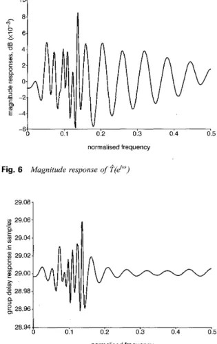
T(ej"), respectively, for the IIR NDF bank designed by the, proposed technique. Finally, the magnitude response of

FJkN - T(eJ") is shown in Fig. 8. From the presented design results, we note that the proposed technique provides very satisfactory performance.

310

Example 2: We use the following design specifications: the

group delay k d is 19; wp = 0.3n and w, = 0.571; Lo = 2 and L l = 3 ; M o = N o = 1 0 a n d M l = N 1 = l l . In the FIR case,

Ho(z) and H ,( z) have orders equal to 32 and 33, respec- tively. Accordingly, the numbers of independent coeffi- cients for the IIR and FIR NDF banks are 44 and 67, respectively. The values o f p and k,,, are the same as those of example 1. Moreover, the values of a,

fl,

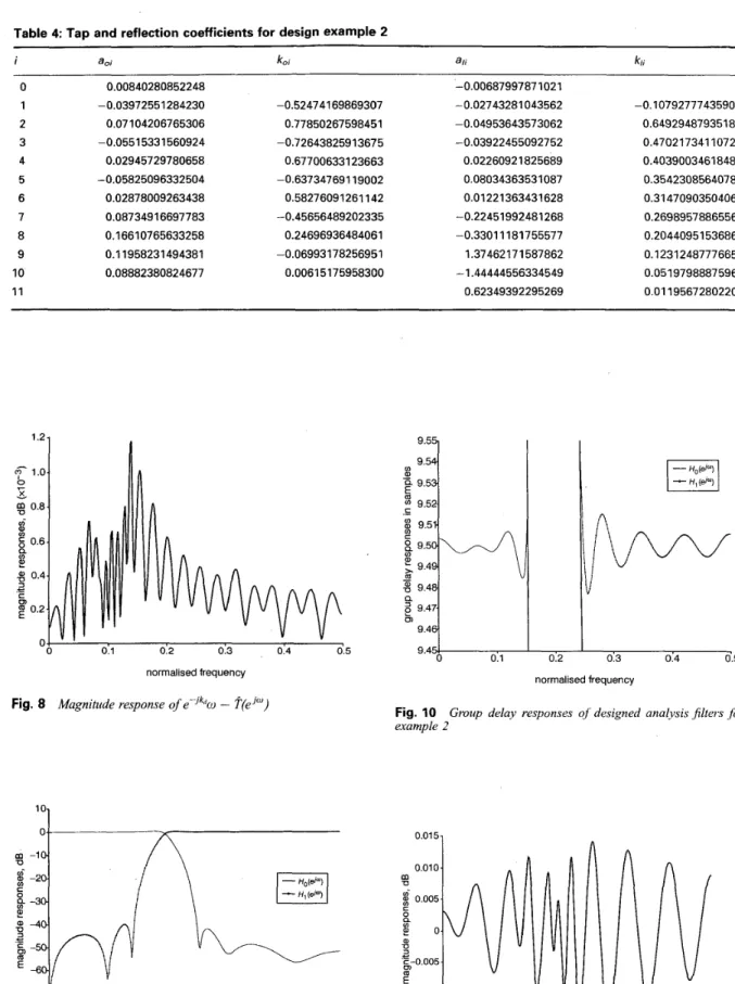
y, y 1 and q2 are set to 0.012, 0.012, 0.055, lo-* and 3.5 x respec- tively, for the design using the proposed technique. The design results with FIR filters using the proposed technique and the results of using the technique [8] to design the same example are also presented for comparison. Table 3 shows the significant design results for the designed NDF banks. The resulting tap and reflection coefficients of the IIR NDF bank obtained after CPU time = 112 s using the proposed technique are given in Table 4. Figs. 9 and 10 plot the corresponding magnitude responses and group delays of Ho(e"")/z/(LLo) and H ~ ( e ' " ) / z / ( L L 1 ) ,

O1

V

0 0.1 0.2 0.3 0.4 0.5

normalised frequency

Fig. 4 Magnitude responses of designed analysis,filters

14.55- * 14.54- g14.53.

E

14.52- a, - m ._

$

14.51 - C 0) X14.50- $14.49- 4 14.40- 2 14.47- 14.46- m

-

a b , I 0.2 14.451 0 0.1 I 1.3 0.4 0.5 normalised frequency

Fig. 5 Group delay responses of analysis jlters

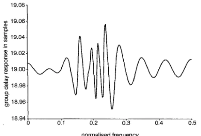
respectively. Figs. 1 1 and 12 depictAthe magnitude response and the group delay response of T(e’”), respectively, for

the IIR NDF bank designed by the proposed technique. Finally, the magnitude response of e-Jkciw - ?(e’“) is

shown in Fig. 13. To show the convergence property of

Table 3: Significant design results for design example 2

m - 4 In $ 2 .< -2 E: g o a, -0 m E -4 -6 0.1 0.2 0.3 0.4 0.5 normalised frequency

Fig. 6 Magnitude response of f(e’(’’)

0 0.1 0.2 0.3 0.4 0.5

28.94

normalised frequency

Fig. 7 Group delay response of ?(e’“)

the proposed technique, Table 5 lists the value of the objective function (1 1) against the iteration number and Fig. 14 depicts the corresponding convergence plot. From the presented design results, we note again that the proposed technique provides very satisfactory performance.

~

IIR NDF bank FIR NDF bank IIR NDF bank o n L2 [81

~ Filter order No. o f coefficients PRE, dB MVGD NPSRo, dB NPSRl, dB MVPGDo MVPGDl SEEO SEE?

Max. variation of filter bank response No. o f iterations 10/10,11/11 44 0.0141 0.0555 32.02 32.03 0.0149 0.0226 3.35 x 10-2 2.22 5.82 x IO-’ 25 32,33 67 0.0172 0.0535 31.07 29.88 0.0113 0.0131 4.80 x IO-’ 7.52 x IO-’ 2.20 IO-^ 51 10/10, 11/11 44 0.0148 0.0583 32.21 32.07 0.0158 0.0230 3.33 x 10-2 2.27 IO-^ 5.68 x IO-’ 37

Table 4: Tap and reflection coefficients for design example 2 9.54 a,

-

_g

9.53

I

9.5) 9.5P .- s! 9.49 m - +! 9.48

g

9.47- a Is) 0 1 2 3 4 5 6 7 8 9 10 1 1 9 . 5 0 4 0.00840280852248 -0.03972551284230 0.07104206765306 -0.05515331560924 0.02945729780658 -0.05825096332504 0.02878009263438 0.0873491 6697783 0.1661 0765633258 0.1 1958231 494381 0.08882380824677 -0.524741 69869307 0.77850267598451 -0.72643825913675 0.677006331 23663 -0.637347691 19002 0.58276091261142 -0.45656489202335 0.24696936484061 -0.06993178256951 0.0061 51 75958300 -0.0068799787 1021 -0.02743281 043562 -0.04953643573062 -0.03922455092752 0.02260921825689 0.08034363531087 0.01 221 363431 628 -0.22451992481268 -0.3301 1181755577 I .37462171587862 -1.44444556334549 0.62349392295269 -0.10792777435909 0.64929487935185 0.470217341 10726 0.4039003461 8481 0.35423085640786 0.31470903504061 0.26989578865561 0.20440951 536865 0.1 2312487776655 0.05197988875961 0.01 195672802207 1.2, 04 ' 0.1 0.2 0.3 0.4 0.5 normalised frequency

Fig. 8 Magnitude response of eYikdm - p(ei'u)

9.4q 9.44 1 . 1 0 0.1 0.2 0.3 0.4 0.5 normalised frequency Fig. 10 example 2

Group delay responses of designed analysis filteis for

10- 0- 0.015 m -10. vi a, -20. 0.010 7J m C 0.005 c

::

9 2 0

;

-30 2 0 -40 a, U ._ 5 -50 c ._ C-0.005 m

2

-60 -70. -0.010 -90. 0.1 0.2 0.3 0.4 0.5 -0.015 0.1 0.2 0.3 0.4 0.5 normalised frequency normalised frequency

Fig. 9 Magnitude responses of designed analysis filters for exam-

ple 2 Fig. 11 Magnitude response of ?(eiw) for example 2

19.08 3 19.06

6

19.04 % 19.02 19.00

0”

18.98 $18.96 18.94 - Q C .- 0 Q - P Q 3 Fig. 12 2.5 - h 2.0-

k

0.1 0.2 0.3 0.4 0.5 normalised frequency

Group delay response of ?(e

’“)

jor example 2

O J

0 0.1 0.2 0.3 0.4 0.5

normalised frequency

Fig. 13 Magnitude response of e-ik@ - ?(eiw) for example 2

Table 5: Convergence property for design example 2

Iteration number Value of objective function (11) 0 (initial) 1 2 3 4 5 6 7 8 9 10 11 12 13 14 15 16 17 18 19 20 21 22 23 24 25 0.6567676534 0.4327604785 0.306631 4681 0.101 8665326 0.0265 105776 0.0242037392 0.02 18806623 0.01953531 38 0.01 43261386 0.0066852773 0.0046182609 0.0023880977 0.0020821327 0.0019039882 0.0018358464 0.0017263049 0.0016922422 0.00 16855382 0.0016449093 0.001 61 779 12 0.001 6097093 0.0015664104 0.001561 1703 0.0015534602 0.0015302981 0.001 5302980

proposed design technique adjusts the tap and reflection coefficients for the analysis filters to reduce the resulting design error and keep the designed IIR analysis filters stable. Simulation results have shown the effectiveness of the proposed technique.

I \

6 Acknowledgment

This work was supported by the National Science Council under grant NSC89-22 13-E002- 162.

iteration number

Fig. 14 Convergence plot for example 2

5 Conclusion

Employing recursive analysis filters with a lattice denomi- nator for designing IIR NDF banks under the L , error criteria has been presented. An approximation scheme has been proposed to solve the resulting highly nonlinear programming problem. The stability of the designed recur- sive analysis filters is ensured by incorporating an efficient stabilisation procedure. Therefore, at each iteration, the

7 References

1 NAYEBI, K., BARNWELL, T.P., and SMITH, M.J.T.: ‘Nonuniform filter banks: a reconstruction and design theory’, IEEE Trans. Signal Process., 1993,41, pp. 1 1 14-1 127

2 WADA, S.: ‘Design of nonuniform division multirate FIR filter banks’,

IEEE Trans. Circuits Syst. II, Analog Digit. Signal Process., 1995, 42,

3 LEE, J.-H., and HUANG, S.-C.: ‘Design of two-channel nonuniform- division maximally decimated filter banks using L , criteria’, IEE Pmc.,

vis. Image Signal Process., 1996, 143, pp. 79-83

4 LEE. J.-H.. and TANG. D.-C.: ‘Outimal desien of two-channel pp. 115-121

nonuniform-division FIR filter banks &th -1, 0, i d +1 coefficients’, IEEE Trans. Signal Process., 1999, 47, pp. 4 2 2 4 3 2

5 EKANAYAKE, M.M., and PREMARATNE, K.: ‘Two-channel IIR QMF banks with approximately linear-phase analysis and synthesis filters’,

IEEE Trans. Signal Process., 1995, 43, pp. 2313-2322

6 TAY. D.B.H.: ‘Desim of causal stable IIR uerfect reconstruction filter banks using transfohation of variables’, IkE Proc., Vis. Image Signal Process., 1998, 145, pp. 287-292

The design of two-channel perfect reconstruction IIR filter banks with causality’, Electron. Commun. Jpn., 1998, 81, pp. 22-31

8 LEE, .I.-H., and NIU, I.-C.: ‘Design of two-channel IIR nonuniform division filter banks with arbitrary group delay’, IEE Proc., Vis. Image Signal Process., 2000, 147, (6), pp. 534-542

7 OKUDA, M., FUKUOKA, T., IKEHARA, M., and TAKAHASHI, S.-I.:

313

9 ADLER, I., KARMARKAR, N., RESENDE, M.G.C., and VEIGA, G.:

‘An implementation of Karmarkar’s algorithm for linear programming’,

Math. Program., 1989, 44, pp. 297-235

network’, IEEE Trans. Acoust. Speech Signal Process., 1984, 32,

pp. 741-749

11 HILLER, F.S., and LIEBERMAN, G.J.: ‘Introduction to mathematical programming’ (McGraw-Hill, New York, 199 1)

12 BELICZYNSKI, B., KALE, I., and CAIN, G.D.: ‘Approximation of FIR by IIR digital filters: an algorithm based on balanced model reduction’,

IEEE Trans. Signal Process., 1992, 40, pp. 532-542

10 LIM, Y.C.: ‘On the synthesis ofIIR digital filters derived from AR lattice 13 OPPENHEIM, A.V., and SCHAFER, R.W.: ‘Discrete-time signal processing’ (Prentice-Hall, Englewood Cliffs, New Jersey, 1989) 14 NELDER, J.A., and MEADE, R.: ‘A simplex method for knction

minimization’, Comput. 1, 1965, 7, pp. 308-313