Pricing the Credit Linked note

全文

(1)Pricing the Credit Linked note. Chou-Wen Wang and Jia-Chiann Chang. Department of Finance National Kaohsiung First University of Science and Technology Tel : 886-7-6011000 ext. 4026 Fax : 886-7-6011401 E-mail : [email protected]. Date:2004/4/10. 第五屆全國實證經濟學論文研討會 The 5th Annual Conference of Taiwan's Economic Empirics.

(2) Abstract We derive a closed-form pricing formula for credit linked notes using reduce-form model. These notes are very popular in European and have been planned to be issued by Taiwan local security firms. These hedge instruments are fixed income security with an embedded credit default swap and can provide the hedge to issuers by the forgiving reference obligation and the issuer has no risk of nondelivery on the hedge. We also use numerical analyses to show that relationship between the volatility of the interest rate, default correlation parameter with interest rate, default intensity that is independent of risk-less spot interest rate and the valuation of credit linked note.. Keywords: credit linked note, default correlation parameter JEL classification: G12,G13. 第五屆全國實證經濟學論文研討會 The 5th Annual Conference of Taiwan's Economic Empirics.

(3) 摘要本文主要利用 reduce-form model 以推導信用連結票券之封閉解。信用連結票券在歐洲近年來相當流行並且台灣政府已開始規劃國內金融機構發行此票券。此信用衍生性商品可視為固定收益證券與信用違約交換以組合而成。此避險工具可使發行者規避標的債權之風險，而且發行者能夠將信用風險完全轉移至票券持有人。本文也進行數值分析以觀察利率波動度、與利率相關之違約相關參數、不受利率影響的違約參數以及信用違約票券價值之間的關係。. 關鍵字: 信用連結票券, 違約相關參數 JEL分類代碼: G12,G13. 第五屆全國實證經濟學論文研討會 The 5th Annual Conference of Taiwan's Economic Empirics.

(4) 1. Introduction In the early 1990s, some countries, such as Latin American, Thailand, Korea and Taiwan, occurred the Asian financial crisis to cause companies face bankruptcy crisis. For financials managers, traditional methods for controlling credit risk such as requiring minimum counterparty credit ratings, requiring collateral could not manage credit risk property. A new financial innovation in credit risk management is the credit derivative, which allows financials managers to "short" credit risk so that opens an avenue for protecting against credit deterioration in a specific asset. A survey of the global credit derivatives market conducted by the British Bankers Association (BBA) in 2002 shows the volumes of credit derivatives market will increase huge in the future. In 2002 and 2004, the volumes will reach $1581 billion and $4799 billion, respectively. The percentage of portfolio products and credit-linked obligations are seen to be the second hot product following by the credit default swaps, with 22% of market share by 2001 and 26% of market share by 2004. The biggest participants in the market are banks and insurers as the buyers and sellers of credit protection, respectively, which manage mainly their loan or investment portfolios so that emphasis the one-time transfer of credit risk. A structured credit linked note is one type of credit derivatives that can be used by debt issuers to hedge against the risk of a default by particular company. The company is known as the reference entity and a default by the company is known as a credit event. Credit events could include bankruptcy, any payment default, repudiation or restructuring. Various forms of structured credit linked notes include credit spread linked notes, total return credit linked notes and credit linked notes. The more popular note among them is the credit linked note. The note is settled by either physical delivery or in cash. If the. 1. 第五屆全國實證經濟學論文研討會 The 5th Annual Conference of Taiwan's Economic Empirics.

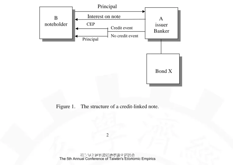
(5) terms of the note require physical delivery, the issuer delivers the bonds to the investor in exchange for their par value. When there is cash settlement, the calculation agent polls dealers to determine the market price of the reference obligation some specified number of days after the credit event. In a credit linked note, the payoff is linked the credit event of reference obligation. An example may help to illustrate how a typical deal is structured. A typical structure of a credit linked note is in Figure 1. Suppose that a bank A issues $10 million nominal of a five-year note referenced to bond B, and the note pays a fixed or floating rate interest. If no credit event occurs on reference obligation, the note will mature at par at the maturity; otherwise the coupon payment eases immediately and the note will be redeemed immediately for the credit event payment (CEP) which could be the market value of reference obligation. Therefore, bank A has received full cash funding from B so that he has hedged its default risk on bond X.. Principal B noteholder. Interest on note CEP. Credit event. A issuer Banker. No credit event. Principal. Bond X. Figure 1. The structure of a credit-linked note.. 2. 第五屆全國實證經濟學論文研討會 The 5th Annual Conference of Taiwan's Economic Empirics.

(6) From the views of the noteholder, the credit linked note’s major advantages include as follows: 1) It can improve capital efficiency, facilitating capital relief from regulators, and opening the door to funding arbitrages. Certain noteholders, notably banks and broker dealers, can reduce capital charges by investing in a credit linked note which issued by a highly-rated borrower and linked to a lower-rated borrower rather than directly investing in a loan or a bond issued by the lower-rated borrower. 2) It enables the noteholder to capture higher value from movements in the value of an underlying loan asset or bond or default risk without the necessity of undertaking a direct investment in the security itself. 3) It provides customized maturity structures and credit features that are linked high yield, non-investment grade security or emerge market which is not otherwise available in the cash market. From the views of the issuers, the structured credit linked note’s major benefits include as follows: 1) the noteholder provides the hedge to issuers by the forgiving reference obligation and the issuer has no risk of nondelivery on the hedge. 2) The issuers can increase the credit line of the reference entity. For example, when the credit line of the reference entity has filled, the bank holding the reference assets can issue the note to transfer potential credit risk and spare the credit line of the reference entity. 3) The note can provide lower-rated companies with a new channel of raising funds. For example, for a lower-rated subsidiary company, it isn’t easy to raise funds itself. Therefore, a higher-rated parent company can issuer a credit linked note that is linked to the performance of a subsidiary company to raise funds. There are a number of variations on the standard credit default linked note. In principal-protected credit linked notes, the payoff protects the noteholder receives 100%. 3. 第五屆全國實證經濟學論文研討會 The 5th Annual Conference of Taiwan's Economic Empirics.

(7) of the notional principle but no additional coupon payment if a credit event occurs. Although issuers just can hedge partial credit risk, it can raise credit rating from non-investment grade to investment grade. Therefore, it is very popular in European. In boosted coupon notes, the payoff of the noteholder arises a multiple growing through the effect of multiple leverage, otherwise may loose the full notional principle. In reduce coupon notes, the payoff is similar to principal-protected credit linked notes. That is the noteholder can receive partial or full notional principle if a credit event occurs. Black and Scholes (1973) and Merton (1974) have been the pioneers in the pricing of corporate bonds using a contingent claim framework. They modelled corporate equity as options on the total value of the firm. Default occurs when the debt expires and when the firm exhausts its assets. As well as we know, C. H. HUI and C. F. LO (2002) are the only one article to derive the credit default linked note up to now. They extend Merton’s corporate bond pricing model to value credit default linked notes by incorporating the value of the reference obligation as an addition variable. Further, they study the effect of the correlation between the values of the note issuer and the reference obligation on credit risk arising from holding credit default linked notes. In practice, however, this valuation methodology is difficult to use because the firm’ value is not observable. Another approach is the reduced-form models in which default time is a stopping time of some given hazard rate process and the payoff upon default is specified exogenously. This approach has been considered by Jarrow and Turnbull (1995), Lando (1994,1998), Duffe and Singleton(1999) and Jarrow and Yu (2001). In this paper, we derive credit linked notes. For credit default linked notes, their formulas are derived in the context of the reduced form credit risk model from Lando. 4. 第五屆全國實證經濟學論文研討會 The 5th Annual Conference of Taiwan's Economic Empirics.

(8) (1998) where correlated defaults arise due to the fact that a firm’s default intensities depend on the common macro-factors. The common macro-factor used in our paper is the spot rate of interest. The spot rate of interest is assumed to follow an extended Vasicek model in the HJM framework. An outline of the article is as follows: We describe the model in Section 2. We derive the closed-form solutions of credit linked note in Section 3. In Section 4, we present the numerical results of the credit linked note. A brief summary and conclusion is offered in Section 5.. 5. 第五屆全國實證經濟學論文研討會 The 5th Annual Conference of Taiwan's Economic Empirics.

(9) 2. Model of Pricing Credit Linked Note We first study the pricing of credit derivatives using the approach of Lando (1998). This is the assumption that facilitates the construction of the doubly stochastic Poisson processes. of. default. (also. called. a. Cox. process). with. an. intensity. function λ ( t , X t ) . {X t : t ∈ [ 0 ,T ]} is right continuous with left limits and a vector stochastic process representing the state variables underling the evolution of the economy and a unit exponential random variable E1 which is independent of X and λ is a non-negative and continuous deterministic intensity function. Let the default time τ as follows:. ⎧. t. ⎫. ⎩. 0. ⎭. τ = inf ⎨t : ∫ λ( X s )ds ≥ E1 ⎬ This default time can be thought of as the first jump time of a Cox process with intensity process λ ( X t ) . In other words, Lando’s reduced-form model allows for dependency between credit and market risk through the use of a Cox process. In a Cox process, these macro-economic state variables induce the correlation between market and default risk. The state variables will include interest rates on riskless debt, time, stock prices, credit ratings and other variables deemed relevant for predicting the likelihood of default. For example, if X t quantifies market risk and λ ( t , X t ) increases as X t increases, then as market risk increases, the likelihood of the firm defaulting increases as well. The filtration is generated collectively by the information contained in the state variables and the default processes: Ft = Gt ∨ H t. 6. 第五屆全國實證經濟學論文研討會 The 5th Annual Conference of Taiwan's Economic Empirics.

(10) Where Gt = σ ( X s ,0 ≤ s ≤ t ) and H t = σ ( 1{τ ≤ s} ,0 ≤ s ≤ t ). Ft then corresponds to knowing the evolution of the state variables up to time t and whether. default. has. occurred. or. Also λ( t , X t ) is Gt measurable. not.. and. t. * satisfies ∫ λ s ds < ∞ , for all t ∈ [ 0,T ] .Therefore, the conditional and unconditional 0. distributions of τ are given by t. P (τ > t ( X s ) 0≤ s ≤t ) = exp(− ∫ λ ( X s ) ds ) , t ∈ [ 0 ,T * ] 0. t. and P (τ > t ) = E exp(− ∫ λ ( X s ) ds ) , t ∈ [ 0 ,T * ] 0. Under the assumption of no arbitrage and complete markets, standard arbitrage pricing theory implies that there exists a unique equivalent probability P such that the present values of the zero-coupon bonds are computed by discounting at the spot rate of interest and then taking an expectation with respect to P. That is, t. B(t ) = exp( ∫ rs ds ) 0. p( t ,T ) = E(. B( t ) Ft ) B( T ). Where p( t ,T ) represents the time t price of a default-free dollar paid at time T, 0 ≤ t ≤ T The cash flows from most credit derivatives can be decomposed into three different claims: (i) The first is a random payment X 1{τ >T } ∈ GT at time T, but only if there is no default. 7. 第五屆全國實證經濟學論文研討會 The 5th Annual Conference of Taiwan's Economic Empirics.

(11) prior to time T. (ii) The second is a random payment rate Ys 1{τ > s} specified by the Gt －adapted process Y which stops when default occurs for the period [0,T]. (iii) The third is a random payment that occurs only at default of Z τ where Z is a Gt － adapted process, zero otherwise. This payment is made only if default occurs during the time period [0,T]. Under appropriate integrability conditions, the present values of these credit risky cash flows are: T. T. 0. 0. (i) E (exp(− ∫ rs ds ) X 1{τ >T } Ft ) = 1{τ >T } E (exp(− ∫ (rs + λ s ) ds ) X ) Ft T. s. T. s. t. t. t. t. (ii) E ( ∫ Ys 1{τ > s} exp(− ∫ ru du ) ds Ft ) = 1{τ >t } E ( ∫ Ys exp(− ∫ (ru + λu )du )ds Ft ) τ. T. s. t. t. t. (iii) E (exp(− ∫ rs ds ) Zτ Ft ) = 1{τ >t } E ( ∫ Z s λ s exp(− ∫ (ru + λu )du )ds ) Ft ) The proof is in the appendix B. According to the previous literature, Duffee’s (1999) uses the bond data to estimate a reduced form credit risk model where both the default intensity and the default free term structure follow a square root process. He finds that the default intensity also depends on the spot rate of interest, so his model captures correlated defaults. Janosi, Jarrow, Yildiray (2000) are different from Duffee (1999), which their default intensity also depends on the cumulative excess return per unit of risk on an equity market index. He found that this added no additional explanatory power in the pricing of corporate debt. Hence, to obtain a simple, but realistic empirical formulation of the following model, we. 8. 第五屆全國實證經濟學論文研討會 The 5th Annual Conference of Taiwan's Economic Empirics.

(12) assume that the point processes governing default are dependence of the risk-free spot interest rate and the risk-free spot interest rate is the only state variable. We assume a linear function: λ ( u ) = λ0 ( u ) + λ1 r( u ) where λ0 (u ) is default intensity that is. independent of risk-less spot interest rate and λ1 (u ) is default correlation with interest rate. For the spot rate of interest, we use a single factor model with deterministic volatilities, sometimes called the extended Vasicek model.. 9. 第五屆全國實證經濟學論文研討會 The 5th Annual Conference of Taiwan's Economic Empirics.

(13) 3. Pricing the Credit Linked Note The credit default linked note lasts for a fixed period of time [0,T ], T is the note’s maturity and τ is the credit event determination date. We define C s is the coupon payment and M is the principle account and δ τR is an amount equal to the recovery rate payment of reference obligation. The valuation of the credit linked note is given by. ⎡T B( t ) R ⎤ B( t ) B( t ) δ τ Ft ⎥ M 1{τ >T } + 1{τ > s} + C( t ) = E ⎢ ∫ C s B ( τ ) B ( T ) B ( s ) ⎣t ⎦ We provide the closed-form solution of the credit linked note in Theorem 2.. Theorem 1 The closed-form pricing formula of the credit linked note is as follows: T. T. T. C (t ) = 1{τ >t } ∫ C s G1 (t , s ) ds + 1{τ > t } MG 1 (t , T ) + ∫ δ λ0 ( s )G1 (t , s) ds + ∫ δ sR λ1G2 (t , s) ds R s. t. t. t. Where. ⎤ ⎡ (1 + λ1 ) 2 2 exp ⎢− λ0 (i − t ) − (1 + λ1 )u (t , i ) + σ (t , i)⎥ = G1 (t , i) , i = s or T 2 ⎦ ⎣ ⎡ ⎤ (1 + λ1 ) 2 2 exp⎢− λ0 (s − t ) − (1 + λ1 )u(t, s) + σ (t, s)⎥ u0 (t, s) − (1 + λ1 )b(t, s) 2 = G2 (t, s) 2 ⎣ ⎦. [. The proof of Theorem 1 is shown in Appendix C.. 10. 第五屆全國實證經濟學論文研討會 The 5th Annual Conference of Taiwan's Economic Empirics. ].

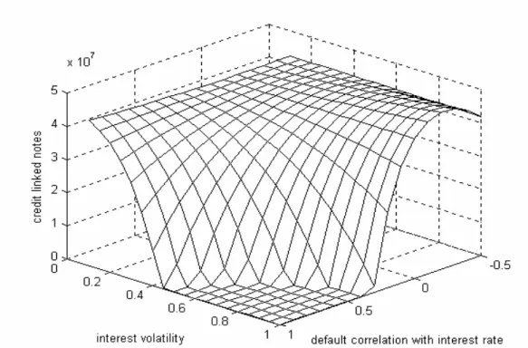
(14) 4. Numerical Analyses of the Credit Default Linked Note In this section, we investigate the properties of the credit linked note numerically under the Vasicek model of short-term rate which is a special case of the HJM framework. Taking a two-year credit linked note issued by Deutsche Australia Ltd guaranteed by Deutsche Bank AG Sydney Branch on November 1, 2001 as an example, the principle amount is AUD 40,000,000 per note and the maturity date is August 1, 2003. The reference entity is Leighton Holdings Limited. Credit Event Monitoring Agent and Calculation Agent is Deutsche Bank AG Sydney Branch. The coupon is 3-mouth BBSW is 5%, which is payable quarterly. If a credit event occurs, no further interest will be calculated or paid from the interest payment date. At maturity, the investors receive AUD 40,000,000 unless a credit event occurs, in which case they receive a credit event settlement amount equal to the nominal amount times recovery rate δ R (t ) .For simplicity, we assume that a =0.02, δ R (t ) is constant equal to 0.4* AUD 40,000,000, riskless pure bond’s price=0.95. Figure 2 show that relationship between the volatility of the interest rate σ r , default correlation with interest rate λ1 (u ) and the valuation of credit linked note. We see that when λ1 (u ) <0, the value of credit linked note is increasing with the volatility. of the interest rate. If λ1 (u ) >0, the value of credit linked note decreases with the increase of the volatility of the interest rate. In practice, this result is consistent with Duffee (1996) that find the negative correlations between default-free interest rates and bond yield spreads. In theorem model, Longstaff and Schwartz (1995) and Jarrow and Yu (2001) also find that when λ1 (u ) is positive, a higher spot rate will lead to a higher yield spread. In Figure 3, assume that we extend the maturity one year from two years to three years,. 11. 第五屆全國實證經濟學論文研討會 The 5th Annual Conference of Taiwan's Economic Empirics.

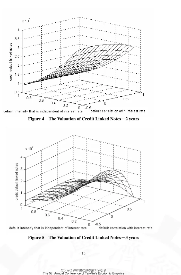
(15) then the result is more significant. In figure 4, we show that relationship between the default intensity that is independent of risk-less spot interest rate λ0 (u ) , default correlation with interest rate λ1 (u ) and the valuation of credit linked note. We see the negative correlations between λ0 (u ) and the valuation of credit linked note. When λ1 (u ) <0, the value of credit linked note is increasing. If λ1 (u ) >0, the value of credit linked note is decreasing. In Figure 5, assume that we extend the maturity one year from two years to three years, we can find this result is more significant. When λ1 (u ) >0, the value of credit linked note decreases fast.. 12. 第五屆全國實證經濟學論文研討會 The 5th Annual Conference of Taiwan's Economic Empirics.

(16) 5. Conclusions In this paper, we derive a closed-form pricing formula for credit linked notes using reduce-form model. These notes are very popular in European and have been planned to be issued by Taiwan local security firms. These hedge instruments can provide the hedge to issuers by the forgiving reference obligation and the issuer has no risk of nondelivery on the hedge. The numerical results show that when λ1 is positive, the value of credit linked note is increasing with the volatility of the interest rate. If λ1 is negative, the value of credit linked note decreases with the increase of the volatility of the interest rate. Further, we see the negative correlations between λ0 and the valuation of credit linked note.. 13. 第五屆全國實證經濟學論文研討會 The 5th Annual Conference of Taiwan's Economic Empirics.

(17) Figure 2 The Valuation of Credit Linked Notes－2 years. Figure 3 The Valuation of Credit Linked Notes－3 years. 14. 第五屆全國實證經濟學論文研討會 The 5th Annual Conference of Taiwan's Economic Empirics.

(18) Figure 4 The Valuation of Credit Linked Notes－2 years. Figure 5 The Valuation of Credit Linked Notes－3 years. 15. 第五屆全國實證經濟學論文研討會 The 5th Annual Conference of Taiwan's Economic Empirics.

(19) Appendix 1 The Extended Vasicek Model within the HJM Framework To fully utilize the tools developed for the HJM term structure model, we specify a forward rate process that is consistent with the extended Vasicek spot rate model. dr (t ) = a(r (t ) − r (t ))dt + σ r ⋅ dWt Where Wt is a Wiener process under the equivalent martingale measure P, and r( t ) is a deterministic function chosen to fit an initial term structure, with a and σ r constants. The solution to equation above is t. t. 0. 0. r (t ) = r (0)e − at + ∫ e a ( s −t ) a r ( s )ds + ∫ e a ( s −t )σ r ⋅ dW ( s ) Where σ ( t ,T ) = e − a( T −t )σ r. df ( t ,T ) = α ( t ,T )dt + σ ( t ,T ) ⋅ dWt Using HTM drift restriction under the risk-neutral measure (P * ), the drift process is related to the volatility by T. α ( t ,T ) = σ ( t ,T )∫ σ ( t , s )ds = a. a ( t −T ). t. T. σr ⋅∫e. a (t −s ). σ r ds = e. a ( t −T ). ⋅σ r. t. = e a( t −T ) ⋅ σ r. 2. e a ( t −T ) − 1 −a. e a( t −T ) − 1 σ r a (t −T ) = e (1 − e a ( t −T ) ) −a a 2. 2. Using the time-t forward rate curve, one gives an alternative expression for the spot rate: s. s. t. t. f ( t , s ) = r( s ) = f ( t ,t ) + ∫ α ( v ,t )dv + ∫ σ ( v ,t ) ⋅ dW ( v ) s. Where ∫ α ( v ,t )dv = t. =. σr2 a. s. ∫e. a ( v −t ). (1− e. )=. t. σ r 2 ⎡ 1 − e − a( s −t ) ⎢ a ⎣. Hence, r( s ) = f ( t , s ) +. a ( v −t ). a. σr2 2a. σr2 ⎡. s. ⎢⋅ e a ⎣ ∫t. a ( v −t ). ⎤ − ∫ e 2 a ( v −t ) ⎥ t ⎦ s. 1 − e −2 a ( s − t ) ⎤ σ r − ( 1 − e − 2 a( s −t ) ) 2 ⎥= 2 a ⎦ 2a 2. s. ( 1 − e − a( s −t ) ) 2 + ∫ e − a( v −t )σ r ⋅ dW ( v ) 2 t. 16. 第五屆全國實證經濟學論文研討會 The 5th Annual Conference of Taiwan's Economic Empirics.

(20) = f ( t ,s ) +. s. b( t , s ) 2 + ∫ β ( v , s ) ⋅ dW ( v ) 2 t s. Where β ( v , s ) = σ r e − a( s −v ) , b( t , s ) = ∫ β ( v , s )dv =. σ r ( 1 − e − a ( s −t ) ) a. t. Thus its mean and variance are E t ( r( s )) = f ( t , s ) +. b( t , s ) 2 ≡ u0 ( t , s ) 2. (A1). s. Var( r( s )) = ∫ β ( v , s ) 2 dv ≡ σ 2 ( t , s ). (A2). t. T. To calculate. ∫ r (u )du, we use the time- t. forward rate curve, then. t. T. T. T. u. T. u. t. t. t. t. t. t. ∫ r (u )du = ∫ f (t , u )du + ∫ du ∫ α (v, u )dv + ∫ du ∫ σ (v, u )dW (v) T. T. t. t. T. T. = ∫ f (t , u )du + ∫ du = ∫ f (t , u )du + ∫ du t. t. T. T. t. t. σ r 2 (1 − e − a (u −t ) ) 2 2a 2. σ r 2 (1 − e − a ( u −t ) ) 2 2a. = ∫ f (t , u )du + ∫ du ⋅ Where b( u ,T ) = T. T. ∫. E( r( u )du ) = t. ∫ t. σr a. 2. T. T. t. v. T. σr. + ∫ dW (v) ∫ σ (v, u )du + ∫ dW (v) t. a. (1 − e −a (T −v ) ). T. b(u , T ) 2 + ∫ dW (u )b(u , T ) 2 t. (1 − e − a (T −u ) ) Thus its mean and variance are T. T. b( u ,T )2 b( u ,T )2 du ≡ u( t ,T ) du = − ln p( t ,T ) + f ( t ,u )du + 2 2 t t. ∫. ∫. T. T. t. t. Var( ∫ v( u )du ) = ∫ b( u ,T ) 2 du ≡ σ 2 ( t ,T ) s. s. s. s. t. t. t. t. (A3). (A4). cov( r( s ), ∫ r( u )du ) = Et ( r( s )∫ r( u )du ) = ∫ β ( v , s )dW ( v )∫ b( v , s ) ⋅ dW ( v ) s. = ∫ β ( v , s )b( v , s )d ( v ) = b( t , s ) 2 t. 17. 第五屆全國實證經濟學論文研討會 The 5th Annual Conference of Taiwan's Economic Empirics. (A5).

(21) Appendix 2 Proof of three basic building blocks in defaultable contingent claims T. T. t. t. (1) E (exp(− ∫ rs ds ) X 1{τ >T } Ft ) = 1{τ >t } E (exp(− ∫ (rs + λ s )ds ) X ) Ft ) Using the law of iterated conditional expectations: T T ⎛ ⎞ E (exp(− ∫ rs ds ) X 1{τ >T } Ft ) = E ⎜⎜ E (exp(− ∫ rs ds ) X 1{τ >T } GT ∨ H t ) Ft ⎟⎟ t t ⎝ ⎠. ⎛ B (t ) ⎞ = E ⎜⎜ XE (1{τ >T } GT ∨ H t ) Ft ⎟⎟ ⎝ B(T ) ⎠ Where E (1{τ >T } GT ∨ H t ) = P (τ > T GT ∨ H t ) We use the fact that the conditional expectation is clearly 0 on the set {τ ≤ t}and that the set {τ > t} is an atom of H t . P (τ > T GT ∨ H t ) = 1{τ >t } P (τ > T GT ∨ H t ) T. = 1{τ >t }. P (τ > T ,τ > t GT ) P (τ > T ,τ > t GT ). = 1{τ >t }. exp(− ∫ λ ( X s )ds ) 0 t. exp(− ∫ λ ( X s )ds ). T. = 1{τ >t } exp(− ∫ λ ( X s )ds ) t. 0. Therefore, T. T. B (t ) X 1{τ >t } exp(− ∫ λ ( X s )ds ) Ft ) E (exp(− ∫ rs ds ) X 1{τ >T } Ft ) = E ( B (T ) 0 t T. (B.1). = 1{τ >t } E (exp(− ∫ (rs + λ s )ds ) X ) Ft ) t. T. s. T. s. t. t. t. t. (2) E ( ∫ Ys 1{τ > s} exp(− ∫ ru du ) Ft ) = 1{τ >t } E ( ∫ Ys exp(− ∫ (ru + λu )du )ds Ft ) Using the law of iterated conditional expectations: T. s. T. s. t. t. t. t. E ( ∫ Y s 1{τ > s } exp( − ∫ ru du ) Ft ) = E ( ∫ 1{τ > t } exp( − ∫ ( ru + λ u )du )Y s ds Ft ) T. s. = 1{τ > t } E ( ∫ Y s exp( − ∫ ( ru + λ u ) du )Y s ds F t ) t. t. 18. 第五屆全國實證經濟學論文研討會 The 5th Annual Conference of Taiwan's Economic Empirics. (B.2).

(22) τ. T. s. t. t. t. (3) E (exp(− ∫ rs ds ) Z τ Ft ) = 1{τ >t } E ( ∫ Z s λ s exp(− ∫ (ru + λu )du )ds ) Ft ) For the proof of (3) note that conditionally on GT and for s > t the density of the default time is given by ∂ ⎛ P (τ ≤ s τ > t , GT ) ⎞⎟ ∂ ⎛⎜ P (t < τ ≤ s GT ) ⎞⎟ ∂ = P (τ ≤ s τ > t , GT ) = ⎜⎜ ∂s ⎝ P (τ > t GT ) ⎟⎠ ∂s ⎜⎝ P(τ > t GT ) ⎟⎠ ∂s Then we show that. P (t < τ ≤ s GT ) = P (τ > t GT ) − P(τ > s GT ) t. s. t. s. 0. 0. 0. t. = exp(− ∫ λ ( X u )du ) − exp(− ∫ λ ( X u )du ) = exp(− ∫ λ ( X u )du )(1 − exp(− ∫ λ ( X u )du )) Hence, ∂ ∂ P (τ ≤ s τ > t , GT ) = (1 − exp(− ∫ λ ( X u )du )) = λ ( X s ) exp(− ∫ λ ( X u )du ) ∂s ∂s t t s. s. (B.3). Now consider (3). τ τ u ∞ ⎛ ⎞ E(exp(−∫ rs ds)Zτ Ft ) = E⎜⎜ E(exp(−∫ rs ds)Zτ GT ∨ Ht ) Ft ⎟⎟ = E(∫ exp(−∫ rs ds)Zu f Z du Ft ) t t t t ⎝ ⎠. Where f Z =. (B.4). ∂ P( τ ≤ s τ > t ,GT ) ∂s. At the time t , we have got whether τ > t or not and Z is clearly 0 on the set {τ > T }. Combing (B.1) and (B.2), we conclude that u u ∞ ⎛T ⎞ E ( ∫ exp( − ∫ rs ds ) Z u f Z du Ft ) = E ⎜⎜ ∫ Z u λu exp(− ∫ (rs + λ s )ds )du Ft ⎟⎟ t t t ⎝t ⎠. 19. 第五屆全國實證經濟學論文研討會 The 5th Annual Conference of Taiwan's Economic Empirics.

(23) Appendix 3 Theorem 1. ⎡T B(t ) B(t ) B(t ) R ⎤ M 1{τ >T } + δτ Ft ⎥ 1{τ >s} + C( t ) = E ⎢∫ C s B s B T B τ ( ) ( ) ( ) ⎦ ⎣t. (D.1). We divide (D.1) into three parts:. ⎡T ⎤ B( t ) 1{τ >s} Ft ⎥ I 1 = E⎢∫ Cs B( s ) ⎣t ⎦ ⎡ B( t ) ⎤ I 2 = E⎢ M 1{τ >T } Ft ⎥ ⎣ B( T ) ⎦ ⎡ B( t ) R ⎤ I3 = E⎢ δ τ Ft ⎥ ⎦ ⎣ B( τ ). To compute I 1 , we use the law of the iterated conditional expectations, then. ⎤ ⎡T B( t ) 1{τ >s} Ft ⎥ E⎢∫ Cs B( s ) ⎦ ⎣t ⎤ ⎡ T B( t ) = E ⎢ E( ∫ C s 1{τ > s} GT ∨ H t ) Ft ⎥ B( s ) ⎦ ⎣ t. ⎤ ⎡T B( t ) = E ⎢∫ C s E( 1{τ > s} GT ∨ H t ) Ft ⎥ B( s ) ⎦ ⎣t Using expression (B.2), we obtain s ⎡T ⎤ B(t ) 1{τ >t } exp( − ∫ λ (u )du ) Ft ⎥ = E ⎢∫ Cs B( s ) t ⎣t ⎦. (D.2). Exchanging the integrals and expectation is justified by Fubini’s theorem(see lamma1) and substitution of the linear intensity λ ( u ) = λ0 ( u ) + λ1 r( u ) into (D.2): T s ⎞ ⎛ = 1{τ >t } ∫ C s E ⎜⎜ exp(− ∫ r (u ) + λ0 (u ) + λ1r (u )du ) Ft ⎟⎟ t t ⎠ ⎝ s ⎤ ⎡ = 1{τ >t } ∫ C s exp(− ∫ λ0 (u )du ) E ⎢exp(−( ∫ (1 + λ1 )r (u ))du ) Ft ⎥ t t t ⎦ ⎣ T. s. 20. 第五屆全國實證經濟學論文研討會 The 5th Annual Conference of Taiwan's Economic Empirics.

(24) s. Because that r is an normal random variable, we let x = exp( − ∫ (1 + λ1 )r (u ) du ) and t. E expx = exp(E( x) + 12 var(x)) . Then, s s ⎤ ⎡ 1 E exp = exp ⎢ E (− ∫ (1 + λ1 )r (u )du ) + 2 var(− ∫ (1 + λ1 )r (u )du )⎥ t t ⎦ ⎣ x. s s ⎤ ⎡ 2 = exp ⎢− (1 + λ1 ) E ( ∫ r (u )du ) + 12 [− (1 + λ1 )] var(∫ r (u )du )⎥ t t ⎦ ⎣. (D.3). Using expressions (A.3)-(A.4) and substitution them into (D.3), we get ⎤ ⎡ (1 + λ1 ) 2 2 = exp ⎢− (1 + λ1 )u (t , s ) + σ (t , s )⎥ 2 ⎦ ⎣ T ⎤ ⎡ (1 + λ1 ) 2 2 σ (t , s )⎥ = 1{τ >t } ∫ C s exp ⎢− λ0 ( s − t ) − (1 + λ1 )u (t , s ) + 2 ⎦ ⎣ t s. s. t. t. Where u( t , s ) = E( ∫ r( u )du ),σ 2 ( t , s ) = var( ∫ r( u )du ) Similarly, for compute I 2 , we use the law of the iterated conditional expectations, then T ⎡ ⎤ E ⎢exp(− ∫ r (u )du ) M 1{τ >T } Ft ⎥ t ⎣ ⎦ T ⎤ ⎡ = E ⎢exp(− ∫ r (u )du ) M E (1{τ >T } GT ∨ H t ) Ft ⎥ t ⎦ ⎣. Using expression (B.1), we obtain T T ⎤ ⎡ = E ⎢ exp( − ∫ r (u ) duM 1{τ > t } exp( − ∫ λ (u ) du ) Ft ⎥ t t ⎦ ⎣. T ⎤ ⎡ = 1{τ >t } ME ⎢exp(− ∫ (r (u ) + λ (u ))du ) Ft ⎥ t ⎦ ⎣ T ⎡ ⎤ = 1{τ > t } ME ⎢ exp( − ∫ ( r (u ) + λ 0 (u ) + λ1 r (u )) du ) Ft ⎥ t ⎣ ⎦. T. T. t. t. = 1{τ >t } M exp(− ∫ λ0 (u )du ) E (− ∫ (1 + λ1 )r (u )du ) Ft ). 21. 第五屆全國實證經濟學論文研討會 The 5th Annual Conference of Taiwan's Economic Empirics.

(25) T. Using the same way, let x = − ∫ (1 + λ1 )r (u )du, E exp x = exp( E ( x) + 12 var( x)) . We get t. = 1{τ >t } M exp(−λ0 (T − t ) − (1 + λ1 )u (t , T ) +. (1 + λ1 ) 2 2 σ (t , T )) 2. To compute I 3 , τ ⎡ ⎤ E ⎢exp(− ∫ r (u )du )δ τR Ft ⎥ t ⎣ ⎦. Using expressions (B.1) and (B.2), we obtain s ⎤ ⎡T R = E ⎢ ∫ δ s λ s exp(− ∫ (r (u ) + λ (u )du )ds Ft ⎥ t ⎦ ⎣t s ⎡T ⎤ = E ⎢ ∫ δ sR [λ0 ( s) + λ1 r ( s)]exp(− ∫ [r (u ) + λ0 (u ) + λ1 r (u )]du )ds Ft ⎥ t ⎣t ⎦. (D.4). We divide (D.4) into two parts and exchange the integrals and expectation is justified by Fubini’s theorem(see lamma2 and lamma3) ⎡ ⎡ s ⎤ ⎤ J 1 = ∫ δ λ0 ( s ) E ⎢exp ⎢− ∫ (r (u ) + λ0 (u ) + λ1r (u ))du ⎥ ds Ft ⎥ t ⎦ ⎣⎢ ⎣ t ⎦⎥ T. R s. ⎡ ⎤ ⎡ s ⎤ J 2 = ∫ δ λ1 E ⎢r ( s ) exp ⎢− ∫ (r (u ) + λ0 (u ) + λ1 r (u ))du ⎥ ds Ft ⎥ t ⎣ t ⎦ ⎣⎢ ⎦⎥ T. R s. To compute J 1 , we use the same way as computing I 1 . Hence, T. J 1 = ∫ δ s λ0 ( s ) exp[−λ0 ( s − t ) − (1 + λ1 )u (t , s ) + t. (1 + λ1 ) 2 2 σ (t , , s )] 2. To compute J 2 , s ⎡ ⎤ J 2 = ∫ δ λ1 exp(− ∫ λ0 (u )du ) E ⎢r ( s ) exp(−1 + λ1 ) ∫ r (u )du )ds Ft ⎥ t t t ⎣ ⎦ T. s. R s. Given ( X ,Y ) is bivariate normal, we have E (exp(aX + bY ) Ft ) = exp(u x a + u y b +. σ x 2 a 2 + 2σ xy ab + σ y 2 b 2 2. )≡z. 22. 第五屆全國實證經濟學論文研討會 The 5th Annual Conference of Taiwan's Economic Empirics. (D.5).

(26) σ x a2 + 2σ xyab + σ y b2 ∂z 2 = E [x exp(aX + bY) Ft ] = exp(ux a + u y b + )(ux + σ x a + σ xyb) ∂a 2 2. 2. (D.6). s. Using expression (D.6) with X = r( s ) , Y = ∫ r( u )du , a = 0 ,b = −( 1 + λ1 ) and expressions t. (A.1)-(A.5),we obtain: s ⎡ ⎤ E ⎢r ( s ) exp(−(1 + λ1 ) ∫ r (u )du )ds Ft ⎥ t ⎣ ⎦ s ⎞ ⎛ ⎞⎛ (1 + λ1 ) 2 2 = exp⎜⎜ − (1 + λ1 )u (t , s ) + σ (t , s ) ⎟⎟ ⎜⎜ E (r ( s ) + cov(r ( s ),−(1 + λ1 ) ∫ r (u )du ) ⎟⎟ 2 ⎝ ⎠⎝ t ⎠. = exp(−(1 + λ1 )u (t , s ) +. (1 + λ1 ) 2 2 σ (t , s )) u 0 (t , s ) − (1 + λ1 )b(t , s ) 2 2. [. ]. Hence, s ⎤ ⎡ ⎡ ⎤ J 2 = ∫ δ λ1 exp(− ∫ λ0 (u )du ) E ⎢r ( s ) exp ⎢− (1 + λ1 ) ∫ r (u )du ⎥ ds Ft ⎥ t t t ⎣ ⎦ ⎦⎥ ⎣⎢ T. s. R s. T. ⎡. t. ⎣. R = ∫ δ s λ1 exp⎢− λ0 (s − t ) − (1 + λ1 )u(t, s) +. ⎤ (1 + λ1 ) 2 2 σ (t, s)⎥ u0 (t, s) − (1 + λ1 )b(t, s) 2 ds 2 ⎦. [. This completes the proof of the Theorem 1.. 23. 第五屆全國實證經濟學論文研討會 The 5th Annual Conference of Taiwan's Economic Empirics. ].

(27) Lemma 1 T ⎤ ⎡ T B (t ) E ⎢∫ C s exp(− ∫ λ (u )du ) ds Ft ⎥ t t B (T ) ⎦ ⎣. Using Chouchy-Schuarz inequality, we can obtain s. s. Et C s exp(− ∫ (r (u ) + λ (u ))du ) ≤ Et (C s ) 2 Et (exp(− ∫ (r (u ) + λ (u ))du ) 2 t. t. s. = C s2 Et (exp(−2∫ (r (u ) + λ (u ))du )) t. s. s. Where E t (exp( − 2 ∫ ( r (u ) + λ (u ))du )) = Et (exp( − 2 ∫ ( λ0 (u ) + (1 + λ1 ) r (u ))du )) t. t. s. = exp(−2λ0 ( s − t )) Et (exp(−2∫ (1 + λ1 )r (u ))du )). (F.1). t. s. Because that r is an normal random variable, we let x = exp( − ∫ (1 + λ1 )r (u ) du ) and t. E expx = exp(E( x) + 12 var(x)) . Then, expression (F.1). = exp(−2λ0 ( s − t ) − 2(1 + λ1 )u (t , s ) + (1 + λ1 ) 2 σ (t , s )) = G (t , s ) By the assumption u (t , s ) and σ (t , s ) are bounded for all t and s . Hence,. ∫. T t. s. Et C s exp(− ∫ (r (u ) + λ (u ))du ) ds ≤ ∫ t. T t. C s2 G (t , s ) ds < ∞. Using Fubini’s theorem, we can obtain T s T s E t ⎡ ∫ C s exp(− ∫ (r (u ) + λ (u ))du )ds ⎤ = ∫ Et ⎡C s exp(− ∫ (r (u ) + λ (u ))du ) ds ⎤ ⎢⎣ ⎥⎦ ⎢⎣ t ⎥⎦ t t t. 24. 第五屆全國實證經濟學論文研討會 The 5th Annual Conference of Taiwan's Economic Empirics.

(28) Lemma 2 T s E ⎡ ∫ δ sR λ 0 ( s ) exp( − ∫ ( r ( u ) + λ 0 ( u ) + λ 1 ( u )) du ) ds F t ⎤ ⎢⎣ t t ⎦⎥. Using Chouchy-Schuarz inequality, we can obtain s s Et δ sR λ0 (s) exp(−∫ (λ(u)) + (1 + λ1 )r(u))du ≤ Et (δ sR λ0 (s))2 Et ⎡exp(−∫ (λ(u)) + (1 + λ1 )r(u))du⎤ ⎢⎣ ⎥⎦ t t. 2. s = δ s2 λ20 ( s) Et ⎡exp(−2∫ (λ0 (u ) + (1 + λ1 )r (u))du)⎤ ⎢⎣ ⎥⎦ t. Using expression (F.1), we get = δ s2 λ20 ( s)G(t , s) By the assumption u (t , s ) and σ (t , s ) are bounded for all t and s . Hence,. ∫. T. t. s. Et δ sR λ0 (s) exp(−∫ (λ(u)) + (1 + λ1 )r(u))du ds ≤ ∫ t. T. t. (δ sR λ0 (s))2 G(t, s) ds < ∞. Using Fubini’s theorem, we obtain T s Et ⎡∫ δ sR λ0 ( s) exp(−∫ (λ (u )) + (1 + λ1 )r (u))du) ds⎤ ⎢⎣ t ⎥⎦ t T s = ∫ Et ⎡δ sR λ0 ( s) exp(− ∫ (λ (u )) + (1 + λ1 )r (u))du) ds⎤ ⎢⎣ ⎥⎦ t t. 25. 第五屆全國實證經濟學論文研討會 The 5th Annual Conference of Taiwan's Economic Empirics.

(29) Lemma 3 T s E ⎡ ∫ δ sR λ1 r ( s ) exp(− ∫ (r (u ) + λ 0 (u ) + λ1 (u ))du ) ds Ft ⎤ ⎢⎣ t ⎥⎦ t. Using Chouchy-Schuarz inequality, we can obtain s s Et δ sR λ1r(s) exp(−∫ (λ(u)) + (1+ λ1 )r(u))du ≤ Et (δ sR rλ1 (s))2 Et ⎡exp(−∫ (λ(u)) + (1+ λ1 )r(u))du⎤ ⎢⎣ ⎥⎦ t t. 2. s = δ s2 λ12 Et (r (s)) 2 Et ⎡exp(−2∫ (λ0 (u) + (1 + λ1 )r (u))du)⎤ ⎢⎣ ⎥⎦ t. Using expression (F.1), we get = δ s2 λ12 (u0 (t, s) 2 + σ 0 (t , s))G(t, s) By the assumption u (t , s ) and σ (t , s ) are bounded for all t and s . Hence,. ∫. T. t. Et δ sR λ1r(s) exp(−∫ (λ(u)) + (1 + λ1 )r(u))du ds ≤ ∫ s. T. t. t. (δ sR λ1 (u0 (t, s) 2 + σ 0 (t, s))G(t, s) ds < ∞ 2. Using Fubini’s theorem, we obtain T s E ⎡ ∫ δ sR λ1 r ( s ) exp(− ∫ (r (u ) + λ0 (u ) + λ1 (u ))du ) ds Ft ⎤ ⎢⎣ t ⎥⎦ t T s = ∫ E ⎡δ sR λ1 r ( s ) exp(− ∫ (r (u ) + λ0 (u ) + λ1 (u ))du ) ds Ft ⎤ ⎢⎣ ⎥⎦ t t. 26. 第五屆全國實證經濟學論文研討會 The 5th Annual Conference of Taiwan's Economic Empirics.

(30) References 1.. Black, F., and J. C. Cox (1976), Valuing corporate securities: Some effects of bond indenture provisions, Journal of Finance, 31, 351-367.. 2.. C.H. Hui and C.F. Lo (2002), Effect of asset value correlation on credit-linked note values, International Journal of Theoretical and Applied Finance, 5(5), 455-478.. 3.. Satyajit Das (2001), Structured products & hybrid securities, New York: Wiley.. 4.. Duffee, Gregory R. (1996), Treasury yields and corporate bond yield spreads: An empirical analysis, Working paper, Federal Reserve Board (Washington, DC).. 5.. Duffe, J. D., and K. J. Singleton (1999), Modeling term structures of defaultable bonds, Review of Financial Studies, 12, 687-720.. 6.. Duffee, G. (1999), Estimating the price of default risk,” The Review of Financial Studies, 12 (1), 197 –226.. 7.. Janosi, T., R. Jarrow, and Y. Yildirim (2002), Estimating expected losses and liquidity discounts implicit in debt prices, Journal of Risk,5 (1), 1 – 39.. 8.. Jarrow, R., and F. Yu (2001), Counterparty risk and the pricing of defaultable securities, Journal of Finance, 56, 1765-1800.. 9.. Jarrow, Robert, and Stuart Turnbull (1995), Pricing derivatives on financial securities subject to credit risk, Journal of Finance, 50, 53–85.. 10. Lando, D. (1994), Three essays on contingent claims pricing, Ph.D. dissertation, Cornell University. 11. Lando, D. (1998), On cox processes and credit risky securities, Review of Derivatives Research, 2, 99-120. 12. Longstaff, Francis A. and Eduardo S. Schwartz (1995), A simple approach to. 27. 第五屆全國實證經濟學論文研討會 The 5th Annual Conference of Taiwan's Economic Empirics.

(31) valuing risky fixed and oating rate debt, Journal of Finance, 50, 789-820. 13. Merton, R.C. (1974), On the pricing of corporate debt: The risk structure of interest rates, Journal of Finance, 29, 449-470. 14. Vasicek, O. (1977), An Equilibrium Characterization of the Term Structure, Journal of Financial Economics, 5, 177-188.. 28. 第五屆全國實證經濟學論文研討會 The 5th Annual Conference of Taiwan's Economic Empirics.

(32)