Solution for flow rates across the wellbore in a two-zone confined aquifer

Solution for Flow Rates across the Wellbore in a Two-Zone

Confined Aquifer

Shaw-Yang Yang

1

and Hund-Der Yeh

2

Abstract: A closed-form solution for transient flow rates across the wellbore in a confined aquifer is derived from a two-zone radial ground-water flow equation subject to the boundary condition of keeping a constant head at the well radius. An aquifer may be considered as a two-zone system if the formation properties near the wellbore are significantly changed due to the well construction and/or well development. An efficient numerical approach is used to evaluate this newly derived solution. Values of the transient flow rate are provided in a tabular form and compared with those obtained by numerical inversion for the Laplace-domain solution. The results show that the two solutions are in good agreement. This newly derived solution can be used not only for predicting the transient flow rate across the wellbore but also for identifying the effects of a skin with a finite thickness on the estimation of transient flow rates in a ground-water system with two different formation properties.

DOI: 10.1061/共ASCE兲0733-9429共2002兲128:2共175兲

CE Database keywords: Flow rates; Ground water; Numerical analysis; Aquifers.

Introduction

The constant-head test is sometimes employed in site character-ization for determining the hydraulic parameters of aquifers with low permeability. During the test, the hydraulic head across the wellbore is kept constant while the transient flow rate into the well is measured.

Carslaw and Jaeger 共1939兲 gave the solutions for heat flow

from the surface of the region bounded internally by a cylinder such as buried pipe and cable, cooling of mine, etc. Tables of numerical values for the heat-flow rate from the surface which are

of practical interest can be seen in Jaeger and Clarke 共1942兲,

Ingersoll et al.共1950兲, and Ingersoll et al. 共1954兲. Based on the

solution given by Smith 共1937兲, Jacob and Lohman 共1952兲

pre-sented a formula describing the flow rate across the wellbore in nonleaky confined aquifers and listed a table of the numerical values for a wide range of the dimensionless flow rate versus

dimensionless time. Hantush 共1962兲 also provided a formula of

ground-water flow through wedge-shaped aquifers, which has the

same form as the solution given by Jacob and Lohman 共1952兲.

Reed共1980兲 and Batu 共1998兲 listed a wide range of values of that formula for dimensionless well discharge versus dimensionless distance or time.

During well construction, a wellbore skin of finite thickness may develop due to the invasion of drilling mud into the adjacent formation or the removal of fine particles from the surrounding

formation by extensive well development; consequently, an oth-erwise homogeneous aquifer may become a two-zone system. The drilling process may therefore produce a positive wellbore skin that has lower hydraulic conductivity than the undisturbed formation. Conversely, thorough well development removes fine particles, e.g., fine silt and clay particles, from the surrounding formation and produces a negative wellbore skin with an

in-creased conductivity. Markle et al. 共1995兲 developed a

finite-element model to analyze the transient flow rate across the well-bore during a constant-head test conducted in a vertical fractured media. Their results show that during a constant-head test the transient flow rate across the wellbore may be affected when a

wellbore skin exists. Chang and Chen 共1999兲 gave the

Laplace-domain solutions of the hydraulic head and the flow rate across the wellbore in a two-zone ground-water system. They presented curves representing specific capacity versus time as part of an

investigation of the influence of a skin共low-permeability zone兲 on

aquifer parameter estimations.

In this study a closed-form solution is derived for transient flow rate across the wellbore when performing a constant-head test in a two-zone confined aquifer system. In addition, we present a numerical evaluation of this solution, which is ex-pressed in a dimensionless form. Numerical values of this solu-tion are verified by comparing with the results of numerical in-version for the Laplace-domain solution using the modified

Crump algorithm共de Hoog et al. 1982兲. This new solution can be

used as a tool to investigate the effects of the presence of a skin with a finite thickness on the estimation of flow rate across the wellbore.

Mathematical Derivations

Two-Zone Radial Flow Equation under Constant-Head Condition

Fig. 1 shows the well and aquifer configurations for a two-zone confined aquifer system. Several assumptions are made for the

solution of hydraulic heads in the confined aquifer; they are 共1兲

1_{Graduate Student, Institute of Environmental Engineering, National}

Chiao-Tung Univ., Hsinchu, Taiwan.

2_{Professor, Institute of Environmental Engineering, National}

Chiao-Tung Univ., Hsinchu, Taiwan.

Note. Discussion open until July 1, 2002. Separate discussions must be submitted for individual papers. To extend the closing date by one month, a written request must be filed with the ASCE Managing Editor. The manuscript for this paper was submitted for review and possible publication on August 18, 2000; approved on July 25, 2001. This paper is part of the Journal of Hydraulic Engineering, Vol. 128, No. 2, February 1, 2002. ©ASCE, ISSN 0733-9429/2002/2-175–183/$8.00⫹$.50 per page.

the aquifer is homogeneous, isotropic, infinite-extent, and with a

constant thickness, 共2兲 the well is fully penetrating with a finite

radius, and共3兲 the initial head is constant and uniform throughout

the whole aquifer. Based on these assumptions, the governing differential equations in terms of the hydraulic head h(r,t) in two-zone formations can be written as

⳵2_h 1 ⳵r2 ⫹ 1 r ⳵h1 ⳵r ⫽ S1 T1 ⳵h1 ⳵t , rw⭐r⭐r1 (1) and ⳵2_h 2 ⳵r2 ⫹ 1 r ⳵h2 ⳵r ⫽ S2 T2 ⳵h2 ⳵t , r1⬍r⬍⬁ (2)

where the subscripts 1 and 2, respectively, denote the wellbore

skin zone and the undisturbed formation zone, h⫽hydraulic head;

r⫽radial distance from the centerline of the well; rw⫽radius of

the well; t⫽time from the start of the test; S⫽storage coefficient;

and T⫽transmissivity.

The hydraulic head is initially assumed to be zero in both the skin and the undisturbed formation, that is

h1共r,0兲⫽h2共r,0兲⫽0, r⬎rw (3) The boundary condition for maintaining a constant head at r

⫽rw is given by

h1共rw,t兲⫽hw for t⬎0 (4)

where hw⫽constant head around the wellbore at any time. As r

→⬁ the hydraulic head tends to zero:

h2共⬁,t兲⫽0 (5)

Between the skin zone and the undisturbed formation the head is continuous

h1共r1,t兲⫽h2共r1,t兲, t⬎0 (6) and there is conservation of mass:

T1 ⳵h1共r1,t兲 ⳵r ⫽T2 ⳵h2共r1,t兲 ⳵r , t⬎0 (7) Closed-Form Solution

The detailed derivations for the solution of hydraulic head in the Laplace domain for the skin and the undisturbed formation

ob-tained by using Laplace transform for Eqs.共1兲–共7兲 are given in

Appendix I and the results for h¯1 and h¯2 are respectively

ex-pressed as h ¯_1⫽hw p ␾1I0共q1r兲⫺␾2K0共q1r兲 ␾1I0共q1rw兲⫺␾2K0共q1rw兲 (8) and h ¯_2⫽hw p 关␾1I0共q1r1兲⫺␾2K0共q1r1兲兴K0共q2r兲 ␾1I0共q1rw兲K0共q2r1兲⫺␾2K0共q1rw兲K0共q2r1兲 (9) where q1 2_⫽pS1 /T1; q2 2_⫽pS2

/T2; p⫽Laplace variable 共Spiegel 1965兲; I0(u) and K0(u)⫽the modified Bessel functions of the first and second kinds of order zero, respectively; and

␾1⫽

冑

S2T2 S1T1 K0共q1r1兲K1共q2r1兲⫺K1共q1r1兲K0共q2r1兲 (10) and ␾2⫽

冑

S2T2 S1T1 I0共q1r1兲K1共q2r1兲⫹I1共q1r1兲K0共q2r1兲 (11)

The functions I1(u) and K1(u) are the modified Bessel functions

of the first and second kinds of order first, respectively.

Applying Darcy’s law at the wellbore, the solution in the

Laplace domain for the flow rate across the wellbore Q¯w can be

obtained as

Q¯w⫽2␲rwT1

再

hwq1关␾1I1共q1rw兲⫹␾2K1共q1rw兲兴

p关␾2K0共q1rw兲⫺␾1I0共q1rw兲兴

冎

(12)

The solution of Eq.共12兲 in the time domain can be obtained by

using the Laplace inversion integral 共Hildebrand 1976兲 as

Qw⫽2␲rwT1

再

2hw ␲

冕

0 ⬁ e⫺共T1/S1兲u2t ⫻A1共u兲B2共u兲⫺A2共u兲B1共u兲 B₁2共u兲⫹B₂2共u兲 du

冎

(13) with A1共u兲⫽

冑

S2T2 S1T1关 J0共r1u兲Y1共kr1u兲Y1共rwu兲 ⫺Y0共r1u兲Y1共kr1u兲J1共rwu兲兴 ⫺关J1共r1u兲Y0共kr1u兲Y1共rwu兲 ⫺Y1共r1u兲Y0共kr1u兲J1共rwu兲兴 (14) A2共u兲⫽

冑

S2T2 S1T1关 Y0共r1u兲J1共kr1u兲J1共rwu兲 ⫺J0共r1u兲J1共kr1u兲Y1共rwu兲兴 ⫺关Y1共r1u兲J0共kr1u兲J1共rwu兲 ⫺J1共r1u兲J0共kr1u兲Y1共rwu兲兴 (15) B1共u兲⫽

冑

S2T2 S1T1关 J0共r1u兲Y1共kr1u兲Y0共rwu兲 ⫺Y0共r1u兲Y1共kr1u兲J0共rwu兲兴 ⫺关J1共r1u兲Y0共kr1u兲Y0共rwu兲 ⫺Y1共r1u兲Y0共kr1u兲J0共rwu兲兴 (16) and

Fig. 1. Schematic diagram of well and aquifer configurations

B2共u兲⫽

冑

S2T2 S1T1关 Y0共r1u兲J1共kr1u兲J0共rwu兲 ⫺J0共r1u兲J1共kr1u兲Y0共rwu兲兴 ⫺关Y1共r1u兲J0共kr1u兲J0共rwu兲 ⫺J1共r1u兲J0共kr1u兲Y0共rwu兲兴 (17)

where Qw⫽flow rate across the wellbore; k⫽

冑

T1S2/T2S1; J0(u)

and Y0(u)⫽the Bessel functions of the first and second kinds of

order zero, respectively; and J1(u) and Y1(u)⫽the Bessel

func-tions of the first and second kinds of order first, respectively. Eq. 共13兲 is the closed-form solution to the transient flow rate across the wellbore in a two-zone ground-water system. Detailed deriva-tions to obtain the solution are shown in Appendix II.

Dimensionless Variables

Defining dimensionless variables ␣⫽T2/T1, ␤⫽S2/S1, ␶

⫽T2t/S2rw

2

, ␳⫽r/rw, ␳1⫽r1/rw, Q¯Dw⫽Q¯w/(2␲T2hw), and

QDw⫽Qw/(2␲T2hw) where ␣ represents the dimensionless

transmissivity,␤ represents the dimensionless storage coefficient,

␶ represents the dimensionless time during the test, ␳ represents

the dimensionless distance from the centerline of the well, ␳1

represents the dimensionless thickness of the skin, Q¯Dw

repre-sents the dimensionless flow rate in the Laplace domain, and QDw

represents the dimensionless flow rate in the time domain. The dimensionless flow rate across the wellbore derived from Eq.共12兲 can be expressed as

Q¯Dw⫽

rwq1关␾1I1共q1rw兲⫹␾2K1共q1rw兲兴

␣p关␾2K0共q1rw兲⫺␾1I0共q1rw兲兴

(18)

Accordingly Eq.共13兲 may be expressed in dimensionless form

as QDw⫽ 2 ␲␣

冕

0 ⬁ e⫺␤␶u2/␣A1⬘共u兲B2⬘共u兲⫺A2⬘共u兲B1⬘共u兲 B₁⬘2共u兲⫹B₂⬘2共u兲 du (19) where A₁⬘共u兲⫽

冑

␣␤关J0共␳1u兲Y1共k␳1u兲Y1共u兲 ⫺Y0共␳1u兲Y1共k␳1u兲J1共u兲兴⫺关J1共␳1u兲Y0共k␳1u兲Y1共u兲 ⫺Y1共␳1u兲Y0共k␳1u兲J1共u兲兴 (20) A₂⬘共u兲⫽

冑

␣␤关Y0共␳1u兲J1共k␳1u兲J1共u兲 ⫺J0共␳1u兲J1共k␳1u兲Y1共u兲兴⫺关Y1共␳1u兲J0共k␳1u兲J1共u兲 ⫺J1共␳1u兲J0共k␳1u兲Y1共u兲兴 (21) B₁⬘共u兲⫽

冑

␣␤关J0共␳1u兲Y1共k␳1u兲Y0共u兲 ⫺Y0共␳1u兲Y1共k␳1u兲J0共u兲兴⫺关J1共␳1u兲Y0共k␳1u兲Y0共u兲 ⫺Y1共␳1u兲Y0共k␳1u兲J0共u兲兴 (22) and B₂⬘共u兲⫽

冑

␣␤关Y0共␳1u兲J1共k␳1u兲J0共u兲 ⫺J0共␳1u兲J1共k␳1u兲Y0共u兲兴⫺关Y1共␳1u兲J0共k␳1u兲J0共u兲 ⫺J1共␳1u兲J0共k␳1u兲Y0共u兲兴 (23) If the aquifer properties are assumed to be constant through the

whole aquifer, then Eq.共19兲, the flow rate across the wellbore in

the dimensionless form, can be reduced to the single-zone

solu-tion presented by Jaeger and Clarke共1942兲 as

Qw 2␲T2hw ⫽_␲42

冕

0 ⬁ e⫺␶u2 关J₀2共u兲⫹Y₀2共u兲兴 du u (24) Numerical Evaluation Bessel Functions

Eq. 共18兲 includes the Bessel functions I0(u), I1(u), K0(u), and

K1(u). Likewise, Eq. 共19兲 contains the integral composing of

J0(u), J1(u), Y0(u), and Y1(u). These functions approximated

by the formulas given in Abramowitz and Stegun 共1964兲 and

Watson共1958兲 are listed in Appendix III. The argument u in these

formulas may be divided into two ranges, 关0,10兴 and 共10,⬁兲 for

I0(u) and I1(u), 关0,2兴 and 共2,⬁兲 for K0(u) and K1(u), and

关0,12兴 and 共12,⬁兲 for J0(u), J1(u), Y0(u), and Y1(u) in order to achieve better accuracy. Besides, these formulas are essentially composed of infinite series and may converge slowly, especially

when u is small. Therefore, the Shanks method 共Shanks 1955;

Wynn 1956兲 is employed to accelerate the convergence when

evaluating the series. Each function in the integrands of Eqs.共18兲

and共19兲 is calculated to ten decimal places, and thus it bears the same degree of accuracy as those listed in Abramowitz and Ste-gun 共1964兲.

Shanks Method

The Shanks transform, also called the ␧ algorithm, consists of a

family of nonlinear sequence-to-sequence transformations

共Shanks 1955兲. Shanks 共1955兲 proved that these transformations are effective when applied to accelerate the convergence of some slowly convergent sequences and may converge some divergent sequences. Examples of the applications of Shanks method in-clude numerical series, the power series of rational and meromor-phic functions, and a wide variety of sequences drawn from inte-gral equations, geometry, fluid mechanics, and number theory 共Shanks 1955兲.

The partial sums, Sn, of an infinite series may be denoted as

Sn⫽

兺

k⫽1

n

ak (25)

where ak is the kth term of the series. Based on the sequence of

partial sums, the Shanks transform may be expressed as 共Wynn

1956兲 ei⫹1共Sn兲⫽ei⫺1共Sn⫹1兲⫹ 1 ei共Sn⫹1兲⫺ei共Sn兲 , i⫽1,2, . . . (26)

where e0(Sn)⫽Snand e1(Sn)⫽关e0(Sn⫹1)⫺e0(Sn)兴⫺1.

It is necessary to set a certain convergence criterion when applying the Shanks transform to evaluate a given series. There-fore, one may define a convergence factor, ERR, as

兩e2i⫹2共Sn⫺1兲⫺e2i共Sn兲兩⭐ERR (27) The sequence of partial sums is terminated when this criterion is met and the infinite series converges to the estimated value of e2i⫹2(Sn⫺1).

Numerical Inversion

In many engineering problems, the Laplace-domain solutions for mathematical models are tractable, yet the corresponding solu-tions in the time domain may not be entirely possible or easily solved. Under such circumstances, a numerical inversion such as

the Stehfest algorithm 共Stehfest 1970兲 or the Crump algorithm

共Crump 1976兲 may be used. Eq. 共18兲 is numerically inverted by

using the modified Crump algorithm共de Hoog et al. 1982兲, which

is based on the␧-algorithm to evaluate the corresponding

diago-nal Pade approximants共IMSL 1987兲.

Gaussian Quadrature

Gaussian quadrature is widely used in performing the numerical integration of a known function. The integration limits of 兰a

b_{f (x)dx are changed from关a,b兴 to 关⫺1,1兴 by a suitable}

transmation of variable when applying Gaussian quadrature. The

for-mula for an n-point Gaussian quadrature may be written as

共Ger-ald and Wheatley 1989兲

冕

⫺1 1 f共␰兲d␰⫽

兺

i⫽1 n Wif共␰i兲 (28)

where Wi⫽weighting factor and ␰i⫽integration point. Values for

Wiand␰ican be found in books on the fields of numerical

meth-ods 共e.g., Burden and Faires 1989; Gerald and Wheatley 1989兲

and the fields of finite element methods共e.g., Reddy 1984;

Bur-nett 1987兲.

Integration Procedures for the Closed-Form Solution

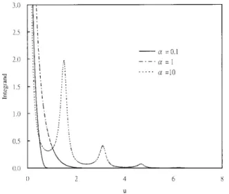
Fig. 2 demonstrates the plots of the integrand of Eq.共19兲 versus u

for ␳⫽1, ␳1⫽3, ␤⫽1, and ␶⫽1 while ␣⫽0.1, 1, or 10. The

two-zone aquifer becomes a homogenous 共single zone兲 aquifer

system when␣⫽1; on the other hand, the aquifer has a negative

skin when ␣⫽0.1 and a positive skin when ␣⫽10. It can be

observed that the integrand of Eq. 共19兲 approaches infinity as u

tends to 0; contrarily, the integrand tends to zero as u becomes very large.

The closed-form solution for the dimensionless flow rate, Eq. 共19兲, cannot be directly evaluated because the integrand contains

a singular point at the origin as indicated in Fig. 2. Letting␧ to be

a very small value, say 10⫺20, and starting from␧, Eq. 共19兲 can be

evaluated by Gaussian quadrature. The initial interval for

numeri-cal integration in Eq.共19兲 is chosen as 10⫺5; then, both six-point

and ten-point formulas of Gaussian quadrature are used at the

same time to carry out the integration of Eq.共19兲. If the difference

of the results by those two formulas is less than the prescribed

criterion, say 10⫺7, a double interval will be used for next

inte-gration. Otherwise, the present interval will be divided into two equal portions, and the same approach is again applied to each

portion until the result for each portion is less than 10⫺7. This

procedure ensures that each result has the accuracy to seven deci-mal places. The same integration procedures are applied to suc-ceeding integrations until the difference in the result for each

portion is less than 10⫺7. Then the remaining integration is

ob-tained by changing the variable as y⫽1/u and the transformed

integral in terms of y is directly evaluated by Gaussian quadrature 共Gerald and Wheatley 1989, p. 304兲. Therefore, the result of nu-merical integrations for the flow rate can be obtained by simply adding all the results from each interval or portion.

Results

Comparisons between the closed-form solution of Eq. 共19兲 and

the results obtained from numerical inversion of Eq. 共18兲 may

provide a cross check for the validity and accuracy of both solu-tions. The values of dimensionless flow rate versus dimensionless time from 0.01 to 1000 evaluated by the proposed numerical

ap-proach for Eq. 共19兲 and the modified Crump algorithm for Eq.

共18兲 are listed in Tables 1 and 2, respectively, for single-zone and two-zone systems. Table 1 gives the values of dimensionless flow

rate versus dimensionless time for␳1⫽3 and ␤⫽1 when ␣⫽1,

that is, when the aquifer formation is under the single-zone con-dition. An approach of infinite series expansion given in

Har-vard’s problem report共1950兲 is adopted to remove the singularity

of the integrand of Eq.共24兲 when performing the integration from

zero to ␧. For the integration limit from ␧ to infinity, Eq. 共24兲 is

evaluated by previously suggested integration procedures. The flow rates estimated by the numerical inversion for the

Laplace-domain solution and those given in Jaeger and Clarke 共1942兲

agree to three decimal places when compared to that of the closed-form solution as shown in Table 1. Table 2 shows the plot

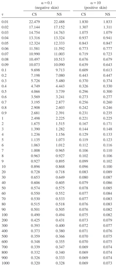
of the dimensionless flow rate versus dimensionless time for ␳1

⫽3 and ␤⫽1 when ␣⫽0.1 or 10. The formation has a negative

skin when␣⫽0.1 and a positive skin when ␣⫽10. The flow rate

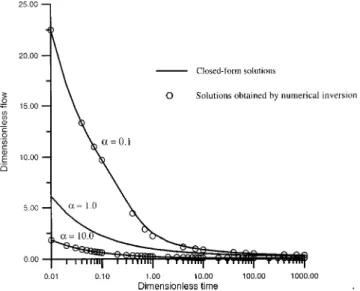
values obtained by numerical Laplace inversion agree well with that of the form solution. This indicates that this closed-form solution yields accurate results for the presence of a well-bore skin when estimated by the proposed numerical approach. Fig. 3 shows that the curve representing the dimensionless flow

rate across the wellbore for the undisturbed共single-zone兲

forma-tion is quite different from that with positive or negative wellbore skin. If a positive wellbore skin exists, then the dimensionless flow rate is smaller than that when a negative wellbore skin exists at the same dimensionless time. A smaller flow rate across the wellbore reflects the result of lower hydraulic conductivity of the positive skin. Conversely, a larger dimensionless flow rate is con-sidered to reflect the increase of formation conductivity and stor-age effects in the presence of a negative wellbore skin.

Conclusions

A closed-form solution for describing the transient flow rate across the wellbore in a two-zone confined ground-water system

Fig. 2. Plot of integrand of Eq. 共19兲 versus u for ␳⫽1, ␳1⫽3, ␤

⫽1, and ␶⫽1 while ␣⫽0.1, 1, or 10

has been developed for the constant-head test with the presence of a wellborn skin. This solution was derived using Laplace trans-form and a contour integral method. In a single-zone aquifer sys-tem, the transient dimensionless flow rates computed from the closed-form solution match well with those given by Jaeger and

Clarke 共1942兲 and the Laplace-domain solution. Under the

two-zone condition, i.e., in the presence of a positive or negative

wellbore skin, the results of the closed-form solution agree with those of the Laplace-domain solution to two decimal places. This provides a double check for the correctness of the closed-form solution.

The flow rate decreases rapidly with increasing time at the early stage of the test and asymptotically approaches a constant value for a long test period. For small times the differences

be-Table 1. Dimensionless Flow Rate versus Dimensionless Time 共␶兲 Estimated by Closed-Form Solution, Numerical Inversion from Laplace-Domain Solution, and One Given in Jaeger and Clarke

共1942兲 for ␳1⫽3 and ␤⫽1 when ␣⫽1 ␶

Closed-form solution

Numerical

inversion solution Jaeger and Clarke

0.01 6.127 6.129 6.219 0.02 4.470 4.472 4.472 0.03 3.735 3.736 3.736 0.04 3.295 3.297 3.297 0.05 2.995 2.997 2.997 0.06 2.773 2.774 2.775 0.07 2.600 2.601 2.602 0.08 2.461 2.462 2.463 0.09 2.345 2.346 2.347 0.1 2.247 2.248 2.249 0.2 1.714 1.715 1.715 0.3 1.475 1.476 1.476 0.4 1.331 1.332 1.333 0.5 1.232 1.233 1.234 0.6 1.159 1.160 1.160 0.7 1.101 1.102 1.102 0.8 1.054 1.056 1.056 0.9 1.015 1.017 1.017 1 0.982 0.984 0.984 2 0.799 0.800 0.800 3 0.715 0.716 0.716 4 0.663 0.664 0.664 5 0.627 0.628 0.628 6 0.599 0.601 0.601 7 0.578 0.579 0.579 8 0.560 0.561 0.562 9 0.545 0.547 0.547 10 0.532 0.534 0.534 20 0.460 0.461 0.461 30 0.425 0.426 0.426 40 0.403 0.404 0.404 50 0.387 0.388 0.388 60 0.375 0.376 0.376 70 0.365 0.366 0.366 80 0.357 0.358 0.358 90 0.350 0.351 0.352 100 0.344 0.346 0.346 200 0.309 0.311 0.311 300 0.292 0.293 0.294 400 0.281 0.282 0.282 500 0.272 0.274 0.274 600 0.266 0.267 0.268 700 0.261 0.262 0.263 800 0.256 0.258 0.258 900 0.253 0.254 0.255 1000 0.246 0.251 0.251

Table 2. Dimensionless Flow Rate versus Dimensionless Time␶ Es-timated by Closed-Form Solution共CS兲 and Numerical Inversion So-lution共NS兲 for ␳1⫽3 and ␤⫽1 when ␣⫽0.1 or 10

␶

␣⫽0.1

共negative skin兲 共positive skin兲␣⫽10

CS NS CS NS 0.01 22.479 22.488 1.830 1.833 0.02 17.144 17.152 1.307 1.311 0.03 14.754 14.763 1.075 1.079 0.04 13.316 13.324 0.937 0.941 0.05 12.324 12.333 0.843 0.847 0.06 11.581 11.592 0.773 0.777 0.07 10.990 11.003 0.719 0.723 0.08 10.497 10.513 0.676 0.679 0.09 10.073 10.090 0.639 0.643 0.1 9.698 9.713 0.609 0.613 0.2 7.198 7.080 0.443 0.447 0.3 5.726 5.480 0.370 0.374 0.4 4.749 4.443 0.326 0.330 0.5 4.066 3.739 0.296 0.300 0.6 3.569 3.241 0.273 0.277 0.7 3.195 2.877 0.256 0.260 0.8 2.908 2.603 0.242 0.246 0.9 2.681 2.391 0.231 0.235 1 2.498 2.225 0.221 0.225 2 1.675 1.515 0.167 0.171 3 1.390 1.282 0.144 0.148 4 1.236 1.156 0.129 0.133 5 1.135 1.073 0.119 0.123 6 1.063 1.012 0.112 0.116 7 1.008 0.965 0.106 0.110 8 0.963 0.927 0.102 0.106 9 0.927 0.895 0.099 0.102 10 0.896 0.868 0.096 0.100 20 0.728 0.718 0.083 0.089 30 0.653 0.649 0.080 0.087 40 0.606 0.605 0.079 0.086 50 0.574 0.575 0.078 0.085 60 0.550 0.552 0.077 0.084 70 0.530 0.533 0.077 0.083 80 0.515 0.518 0.076 0.083 90 0.501 0.505 0.076 0.082 100 0.490 0.494 0.075 0.082 200 0.425 0.431 0.073 0.079 300 0.393 0.400 0.072 0.077 400 0.373 0.380 0.071 0.076 500 0.359 0.366 0.070 0.075 600 0.348 0.355 0.070 0.075 700 0.339 0.347 0.069 0.074 800 0.332 0.340 0.069 0.074 900 0.326 0.333 0.069 0.074 1000 0.320 0.328 0.069 0.073

tween the flow rate in an aquifer with a positive or negative wellbore skin and an aquifer without a wellbore skin are large. In addition, the effect of a negative wellbore skin on the flow rate is larger than that of a positive wellbore skin. Obviously, the mag-nitude of the flow rate across the wellbore strongly depends on the hydraulic properties of both the formation and the wellbore skin.

Acknowledgments

The writers appreciate the comments and suggested revisions of two anonymous reviewers that help improve the clarity of our presentation. Research leading to this paper has been partly sup-ported by the grants from Taiwan Power Company via National Science Council of ROC under Contract No. NSC89-TPC-E-099-001.

Appendix I. Derivation of Eqs. „8… and„9…

Chang and Chen共1999兲 presented the Laplace-domain solutions

of the hydraulic head and the flow rate across the wellbore in a two-zone ground-water system without giving the derivations.

Nevertheless, such solutions in the Laplace domain, Eqs.共8兲 and

共9兲, can be derived based on the procedures given in Carslaw and

Jaeger共1959兲.

Applying the Laplace transform on Eqs.共1兲 and 共2兲 yields

d2_¯h 1 dr2 ⫹ 1 r dh¯1 dr ⫽q1 2_¯h 1 (29) and d2_¯h 2 dr2 ⫹ 1 r dh¯2 dr ⫽q2 2_¯h 2 (30)

Furthermore, Laplace transforms of boundary conditions, Eqs. 共4兲–共7兲, are h ¯_{1⫽hw/ p for r⫽rw (31)} h ¯_{2⫽0 for r→⬁ (32)} h ¯_{1⫽h¯2 for r⫽r1 (33)} and T1 dh¯1 dr ⫽T2 dh¯2 dr for r⫽r1 (34)

The solutions of Eqs.共8兲 and 共9兲 to the hydraulic head in the

Laplace domain in the skin and the undisturbed formation can

then be obtained as共Carslaw and Jaeger 1959兲

h

¯_{1⫽C1I0共q1r兲⫹C2K0共q1r兲 (35)} and

h

¯_{2⫽D1I0共q2r兲⫹D2K0共q2r兲 (36)}

where C1, C2, D1, and D2 are constants.

Substituting Eqs. 共35兲 and 共36兲 into Eqs. 共31兲–共34兲, one can

obtain C1⫽ hw p ␾1 ␾1I0共q1rw兲⫺␾2K0共q1rw兲 (37) C2⫽ hw p ⫺␾2 ␾1I0共q1rw兲⫺␾2K0共q1rw兲 (38) D1⫽0 (39) and D2⫽ hw p ␾1I0共q1r1兲⫺␾2K0共q1r1兲 ␾1I0共q1rw兲K0共q2r1兲⫺␾2K0共q1rw兲K0共q2r1兲 (40)

Consequently, Eq.共8兲 can be obtained by substituting the

con-stants from Eqs. 共37兲 and 共38兲 into Eqs. 共35兲 and 共9兲 can be

obtained by a similar manner. Note that Eq. 共9兲, representing the

head distribution in the undisturbed formation, slightly differs

from the one given in Chang and Chen 共1999兲. Their inaccuracy

may be due to typing errors.

Appendix II. Derivation of Eq. „13…

The inverse Laplace transform of Eq.共12兲 in the time domain can

be obtained by using the Laplace inversion integral 共Hildebrand

1976兲 as Qw⫽ 1 2␲i

冕

_␨⫺i⬁ ␨⫹i⬁ ept_Q¯ wd p (41)

where p⫽complex variable; i⫽imaginary unit; and ␨⫽large,

real, positive constant, so much so that all the poles lie to the left

of the line (␨⫺i⬁,␨⫹i⬁).

A single branch point with no singularity共pole兲 at p⫽0 exists

in the integrand of Eq.共12兲. Thus, this integration may require the

use of the Bromwich integral for the Laplace inversion. The closed contour of the integrand is shown in Fig. 4 with a cut of

the p plane along the negative real axis, where ␦ is taken

suffi-ciently small to exclude all poles from the circle about the origin.

Fig. 3. Results of the closed-form solution evaluated by the numeri-cal approach and the solution obtained from the numerinumeri-cal inversion by using the modified crump approach.

The closed contour consists of the part AB of the Bromwich line from ⫺⬁ to ⬁, semicircles BCD and GHA, lines DE and FG

parallel to the real axis and a circle EF of radius ␦ about the

origin. The integration along the small circle EF around the origin as␦→0 is carried out by using the Cauchy integral and the value of the integration is equal to zero. The integrals taken along BCD

and GHA tend to zero as R→⬁. Consequently, Eq. 共12兲 can be

superseded by the sum of the integrals along DE and FG. In other words, the integral can then be written as

Qw⫽ lim ␦→0 R→⬁ 1 2␲i

冋

冕

DE eptQ¯wd p⫹

冕

FG eptQ¯wd p

册

(42)

For the first term on the right-hand side 共RHS兲 of Eq. 共42兲

along DE we introduce the change of variable p⫽u2e⫺␲iT1/S1

and use the formula共Carslaw and Jaeger 1959, p. 490兲

Kv共ze⫾共1/2兲␲i兲⫽⫾ 1 2␲ie ⫿共1/2兲v␲i_关⫺J v共z兲⫾iYv共z兲兴 (43) and

Iv共ze⫾共1/2兲␲i兲⫽e⫾共1/2兲v␲iJv共z兲 (44)

wherev⫽0,1,2, . . . . The first term on the RHS of Eq. 共42兲 then

leads to Qw1⫽⫺ 2rwT1hw i

冕

0 ⬁ ⫺e共T1/S1兲u2t关A1共u兲⫹iA2共u兲兴 关B1共u兲⫹iB2共u兲兴 du (45)

Likewise, introducing p⫽u2_e␲i_T

1/S1, the integral along EF

gives minus the conjugate of Eq.共45兲 as

Qw2⫽ 2rwT1hw i

冕

0 ⬁ ⫺e共T1/S1兲u2t关A1共u兲⫺iA2共u兲兴 关B1共u兲⫺iB2共u兲兴 du (46)

The closed-form solution of Eq. 共13兲 can then be obtained by

combining Eqs. 共45兲 and 共46兲.

Appendix III. Formulas of Bessel Functions

The Bessel functions of I0(u), I1(u), K0(u), and K1(u) may be

evaluated by the formulas given in Abramowitz and Stegun 共1964兲. The argument u in these formulas can be divided into two

ranges,关0,10兴 and 共10,⬁兲 for I0(u) and I1(u) and关0,2兴 and 共2,⬁兲

for K0(u) and K1(u) for better accuracy. For 0⭐u⭐10, the

asymptotic expansions for I0(u) and I1(u) may be expressed

re-spectively as共Abramowitz and Stegun 1964, p. 375兲

I0共u兲⫽1⫹ 1 4u 2 共1!兲2⫹

冉

1 4u 2

冊

2 共2!兲2 ⫹

冉

1 4u 2

冊

3 共3!兲2 ⫹¯ (47) and I1共u兲⫽

冉

u 2

冊

冋

1⫹ 1 4u 2 共1!兲共2!兲⫹

冉

1 4u 2

冊

2 共2!兲共3!兲⫹

冉

1 4u 2

冊

3 共3!兲共4!兲⫹¯

册

(48)

The Bessel functions of I0(u) and I1(u) for 10⬍u⬍⬁ are

respectively approximated as 共Abramowitz and Stegun 1964, p.

377兲 I0共u兲⫽ eu

冑

2␲u

再

1⫹ 12 共1!兲共8u兲⫹ 12_⫻32 共2!兲共8u兲2⫹ 12_⫻32_⫻52 共3!兲共8u兲3 ⫹¯

冎

(49) and I1共u兲⫽ eu

冑

2␲u

再

1⫺ 4⫺12 共1!兲共8u兲⫹ 共4⫺12兲•共4⫺32兲 共2!兲共8u兲2 ⫺共4⫺1 2_{兲•共4⫺3}2_{兲•共4⫺5}2_兲 共3!兲共8u兲3 ⫹¯

冎

(50)

For 0⭐u⭐2, the asymptotic expansions for K0(u) and K1(u)

may be written respectively as共Abramowitz and Stegun 1964, p.

375兲 K0共u兲⫽⫺

冋

ln

冉

u 2

冊

⫹␥

册

I0共u兲⫹ 1 4u 2 共1!兲2⫹

冉

1⫹ 1 2

冊冉

1 4u 2

冊

2 共2!兲2 ⫹

冉

1⫹ 1 2⫹ 1 3

冊冉

1 4u 2

冊

3 共3!兲2 ⫹¯ (51) and

Fig. 4. Plot of closed contour integration of h¯ for inverse Laplace transform共Hildebrand 1976兲

K1共u兲⫽

冋

ln

冉

u 2

冊

⫹␥

册

I1共u兲⫹ 1 u⫺ u 4

冦

冋

1 4u 2 共1!兲共2!兲⫹

冉

1⫹ 1 2

冊 冉

1 4u 2

冊

2 共2!兲共3!兲⫹

冉

1⫹ 1 2⫹ 1 3

冊 冉

1 4u 2

冊

3 共3!兲共4!兲⫹¯

册

⫹

冋

1⫹

冉

1⫹1 2

冊

1 4 u 2 共1!兲共2!兲⫹

冉

1⫹ 1 2⫹ 1 3

冊 冉

1 4u 2

冊

2 共2!兲共3!兲⫹¯

册

冧

(52)

where␥⫽0.577215664901533 is the Euler’s constant. For 2⬍u⬍⬁, K0(u) and K1(u) are respectively taken as共Abramowitz and Stegun

1964, p. 378兲 K0共u兲⫽ eu

冑

2␲u

再

1⫺ 12 共1!兲共8u兲⫹ 12_⫻32 共2!兲共8u兲2⫺ 12_⫻32_⫻52 共3!兲共8u兲3 ⫹¯

冎

(53) and K1共u兲⫽ eu

冑

2␲u

再

1⫹ 4⫺12 共1!兲共8u兲⫹ 共4⫺12_{兲•共4⫺3}2_兲 共2!兲共8u兲2 ⫹ 共4⫺12_{兲•共4⫺3}2_{兲•共4⫺5}2_兲 共3!兲共8u兲3 ⫹¯

冎

(54)

These functions of J0(u), J1(u), Y0(u), and Y1(u) may be evaluated by the formulas given in Abramowitz and Stegun共1964兲 and

Watson 共1958兲. The argument u in these four functions may be split into two ranges, 关0,12兴 and 共12,⬁兲, for good accuracy. For 0⭐u

⭐12, these functions may be written respectively as 共Abramowitz and Stegun 1964, p. 360兲

J0共u兲⫽1⫺ 1 4u 2 共1!兲2⫹

冉

1 4u 2

冊

2 共2!兲2 ⫺

冉

1 4u 2

冊

3 共3!兲2 ⫹¯ (55) J1共u兲⫽

冉

u 2

冊

冋

1⫺ 1 4u 2 共1!兲共2!兲⫹

冉

1 4u 2

冊

2 共2!兲共3!兲⫺

冉

1 4u 2

冊

3 共3!兲共4!兲⫹¯

册

(56) Y0共u兲⫽ 2 ␲

冋

ln

冉

u 2

冊

⫹␥

册

J0共u兲⫹ 2 ␲

冋

1 4u 2 共1!兲2⫺

冉

1⫹ 1 2

冊冉

1 4u 2

冊

2 共2!兲2 ⫹

冉

1⫹ 1 2⫹ 1 3

冊冉

1 4u 2

冊

3 共3!兲2 ⫺¯

册

(57) and Y1共u兲⫽⫺ 2 ␲u ⫹ 2 ␲

冋

ln

冉

u 2

冊

⫹␥

册

J1共u兲⫹ u 2␲

冦

冋

⫺ 1 4u 2 共1!兲共2!兲⫹

冉

1⫹ 1 2

冊 冉

1 4u 2

冊

2 共2!兲共3!兲⫺

冉

1⫹ 1 2⫹ 1 3

冊 冉

1 4u 2

冊

3 共3!兲共4!兲⫹¯

册

⫹

冋

1⫺

冉

1⫹1 2

冊

1 4u 2 共1!兲共2!兲⫹

冉

1⫹ 1 2⫹ 1 3

冊 冉

1 4u 2

冊

2 共2!兲共3!兲⫺¯

册

冧

(58)

Note that as u⫽0, J0(u) and J₁(u) are equal to one and zero respectively, whereas Y₀(u) and Y₁(u) approach⫺⬁.

The functions of J0(u), J1(u), Y0(u), and Y1(u) for 12⬍u⬍⬁ are approximated respectively as 共Watson 1958, p. 199兲

J0共u兲⫽

冑

2

␲u

再

cos

冉

u⫺ ␲ 4

冊

冋

m

兺

⫽0 ⬁ 共⫺1兲m_{•共0,2m兲} 共2u兲2m

册

⫺sin

冉

u⫺ ␲ 4

冊

冋

m

兺

⫽0 ⬁ 共⫺1兲m_{•共0,2m⫹1兲} 共2u兲2m⫹1

册冎

(59) J1共u兲⫽

冑

2 ␲u

再

cos

冉

u⫺ 3␲ 4

冊

冋

m

兺

⫽0 ⬁ 共⫺1兲m_{•共1,2m兲} 共2u兲2m

册

⫺sin

冉

u⫺ 3␲ 4

冊

冋

m

兺

⫽0 ⬁ 共⫺1兲m_{•共1,2m⫹1兲} 共2u兲2m⫹1

册冎

(60) Y0共u兲⫽

冑

2 ␲u

再

sin

冉

u⫺ ␲ 4

冊

冋

m

兺

⫽0 ⬁ 共⫺1兲m_{•共0,2m兲} 共2u兲2m

册

⫹cos

冉

u⫺ ␲ 4

冊

冋

m

兺

⫽0 ⬁ 共⫺1兲m_{•共0,2m⫹1兲} 共2u兲2m⫹1

册冎

(61) and Y1共u兲⫽

冑

2

␲u

再

sin

冉

u⫺

3␲ 4

冊

冋

m

兺

⫽0 ⬁ 共⫺1兲m_{•共1,2m兲} 共2u兲2m

册

⫹cos

冉

u⫺ 3␲ 4

冊

冋

m

兺

⫽0 ⬁ 共⫺1兲m_{•共1,2m⫹1兲} 共2u兲2m⫹1

册冎

(62) where

共␯,m兲⫽

⌫

冉

␯⫹m⫹1

2

冊

m!⌫

冉

␯⫺m⫹1₂

冊

(63)

and⌫(m) is the Gamma function 共Abramowitz and Stegun 1964, p. 255兲.

References

Abramowitz, M., and Stegun, I. A.共1964兲. Handbook of mathematical

functions with formulas, graphs and mathematical tables, National

Bureau of Standards, Dover, Washington, D.C.

Batu, V.共1998兲. Aquifer hydraulics: A comprehensive guide to

hydrogeo-logic data analysis, Wiley, New York.

Burden, R. L., and, Faires, J. D. 共1989兲. Numerical analysis, 4th Ed., PWS-KENT, Boston.

Burnett, D. S.共1987兲. Finite element analysis, Addison-Wesley, Redwood City, Calif.

Carslaw, H. S., and Jaeger, J. C.共1939兲. ‘‘Some two-dimensional prob-lems in conduction of heat with circular symmetry.’’ Some Probprob-lems

in Conduction of Heat, 46, 361–388.

Carslaw, H. S., and Jaeger, J. C.共1959兲. Conduction of heat in solids, 2nd Ed., Clarendon, Oxford.

Chang, C. C., and Chen, C. S.共1999兲. ‘‘Analysis of constant-head for a two-zone radially symmetric nonuniform model.’’ Proc. 3rd

Ground-water Resources and Water Quality Protection Conf., National Central

Univ., Chung-Li, Taiwan.

Crump, K. S.共1976兲. ‘‘Numerical inversion of Laplace transforms using a Fourier series approximation.’’ J. Assoc. Comput. Mach., 23共1兲, 89– 96.

de Hoog, F. R., Knight, J. H., and Stokes, A. N.共1982兲. ‘‘An improved method for numerical inversion of Laplace transforms.’’ Soc.

Indus-trial Appl. Mathe. J. Sci. Stat. Comput., 3共3兲, 357–366.

Gerald, C. F., and Wheatley, P. O.共1989兲. Applied numerical analysis, 4th Ed., Addison-Wesley, Reading, Mass.

Hantush, M. S.共1962兲, ‘‘Flow of ground water in sands of nonuniform thickness; Park 1. Flow in a wedge-shaped aquifer.’’ J. Geophys. Res., 67共2兲, 703–709.

Harvard Problem Report共1950兲. ‘‘A function describing the conduction of heat in a solid medium bounded internally by a cylindrical sur-face,’’ Computation Laboratory of Harvard Univ. Rep. No. 76.

Hildebrand, F. B. 共1976兲. Advanced calculus for applications, 2nd Ed., Prentice-Hall, Englewood Cliffs, N.J.

Ingersoll, L. R., Adler, F. T. W., Plass, H. J., and Ingersoll, A. G.共1950兲. ‘‘Theory of earth heat exchangers for the heat pump.’’ Heat./Piping/

Air Cond., 113–122.

Ingersoll, L. R., Zobel, O. J., and Ingersoll, A. C.共1954兲. Heat

conduc-tion with engineering, geological, and other applicaconduc-tions, 2nd Ed.,

University Wisconsin Press, Madison, Wis.

International Mathematics and Statistics Library, Inc.共1987兲. IMSL Us-er’s Manual, 2, IMSL, Inc., Houston.

Jacob, C. E., and Lohman, S. W. 共1952兲. ‘‘Nonsteady flow to a well of constant drawdown in an extensive aquifer.’’ Trans., Am. Geophys.

Union, 33共4兲, 559–569.

Jaeger, J. C., and Clarke, M.共1942兲. ‘‘A short table of I(o,i;x).’’ Proc. R.

Soc. Edinburgh, Sect. A: Math. Phys. Sci., 61, 229–230.

Markle, J. M., Rowe, R. K., and Novakowski, K. S.共1995兲. ‘‘A model for the constant-heat pumping test conducted in vertically fractured media.’’ Int. J. Numer. Analyt. Meth. Geomech., 19, 457– 473. Reddy, J. N. 共1984兲. An introduction to the finite element method,

McGraw-Hill, New York.

Reed, J. E.共1980兲. Type curves for selected problems of flow to wells in

confined aquifers; Book 3 applications of hydraulics, United States

Department of the Interior, US GPO, Washington, D.C.

Shanks, D.共1955兲. ‘‘Non-linear transformations of divergent and slowly convergent sequences.’’ J. Math. Phys., 34, 1– 42.

Smith, L. P.共1937兲. ‘‘Heat flow in an infinite solid bounded internally by a cylinder.’’ J. Appl. Phys., 8共6兲, 45–49.

Spiegel, M. R.共1965兲. Laplace transforms, Schaum, New York. Stehfest, H.共1970兲. ‘‘Numerical inversion of Laplace transforms.’’

Com-mun. ACM, 13共1兲, 47–49.

Watson, G. N.共1958兲. A treatise on the theory of Bessel functions, 2nd Ed., Cambridge University Press, Cambridge, U.K.

Wynn, P. 共1956兲. ‘‘On a device for computing the em(Sn) transforma-tion.’’ Math. Tables Aids Comput., 10, 91–96.