流量強度的測量與監控及其在隨機系統控制上之應用

(1)

行政院國家科學委員會專題研究計畫成果報告

流量強度的測量與監控及其在隨機系統控制上之應用

研究成果報告(精簡版)

計畫類別：個別型計畫編號： NSC 100-2118-M-004-005- 執行期間： 100 年 08 月 01 日至 101 年 07 月 31 日執行單位：國立政治大學統計學系計畫主持人：洪英超計畫參與人員：碩士班研究生-兼任助理人員：劉世璿碩士班研究生-兼任助理人員：陳韋成碩士班研究生-兼任助理人員：陳寬旻報告附件：出席國際會議研究心得報告及發表論文公開資訊：本計畫涉及專利或其他智慧財產權，1 年後可公開查詢中華民國 101 年 10 月 20 日

(2)

中文摘要：建構複雜隨機系統的最佳控制策略常常必須仰賴所觀測到的輸入流量強度。但是因為流量強度變動所引起的高操作成本，執行此一類型的控制策略在實際上往往不可行。此計畫中我們將提出一個測量與監控輸入流量強度的架構。此架構完全不需要知道任何輸入過程的統計量，借由即時估計流量強度及同時監控其顯著的變動，最佳控制策略將可以在低操作成本下進行調整。最後，考慮不同的輸入流量類形，我們在一個重要的排隊系統上評估此架構之效益。中文關鍵詞：控制策略；排隊系統；管制圖

英文摘要： The development of optimal control strategies for many complex stochastic systems relies on the observed intensity function of input traffic.

However, implementation of such control strategies is often infeasible due to high operating costs induced by the fluctuations of traffic flows. In this

proposal, we introduce a general framework for

measuring and monitoring the traffic flow intensities of stochastic systems. The framework does not require knowledge of any input traffic statistics and, it allows us to be able to estimate the intensity function over time and simultaneously detect

significant traffic fluctuations so that the control strategy can be adjusted accordingly without

requiring high operating costs. Finally, a canonical queueing system with various types of input traffic is used to evaluate the effectiveness of the proposed framework.

(3)

1

報告內容

(一) 前言

(4)

2 (二) 研究目的

(三) 文獻探討

Comprehensive statistical procedures have been extensively developed for the output analysis of queueing systems. For example, Asmussen (1990) [2] intro-duced an effective Monte Carlo approach involving importance sampling as well as linear regression for studying the mean and other functionals of queues; Hung et al. (2003) [20] developed a framework of efficient simulations for complex queue-ing systems by utilizqueue-ing the idea of treed models and optimum design; Wieland et al. (2003) [38] proposed a simulation-based procedure for checking the stability of queues by utilizing the idea of statistical hypothesis testing; Kleijnen (1992) [22] introduced a regression model for analyzing the input-output behavior of the underlying complicated simulation model; Cheng and Kleijnen (1999) [6] uti-lized the idea of optimum design to determine the traffic intensities at which the queueing systems are simulated so as to improve the proposed regression model for estimating the mean response of interest; just to name a few. The study of measurement based optimal resource allocation problems for queueing systems is rather limited, for which some can be found in the recent works by Hayel et al. (2007) [16], Hung and Michailidis (2006) [17], Kallitsis et al. (2009) [21], and Xu et al. (2006) [39]. It should be highlighted that the work in this study, to the best of our knowledge, is the first attempt to integrate the statistical online estimation and monitoring strategies into the control formulation. In addition to queueing systems, it can be extensively applied to any stochastic models with similar flow analogies and control schemes, such as material flow control in the design of pro-duction lines [13], control of flow cytometry in cell biology [11, 5, 34], control of semi-active suspensions for vehicles or shock and vibration isolation systems [4], just to name a few.

The remainder of this paper is organized as follows. In Section 2, the frame-work based on the EWMA smoothing technique and the control chart used for monitoring the shifts of the estimated traffic intensity is introduced. In Section 3, a motivated fluid control problem for the queueing system under consideration is introduced. Further, the proposed framework is illustrated and its performance evaluated on a number of systems with various types of input traffic flows via a simulation study. Some concluding remarks are drawn in Section 4.

2. Framework for Estimation and Shift-Monitoring of Traffic Intensity Suppose that the optimal control policy of the stochastic system requires knowl-edge of traffic intensities. This implies that for systems with time-varying traffic intensities, the control policy has to be more responsive to traffic fluctuations in

(5)

3

(四) 研究方法

Estimation of Traffic Intensity

Comprehensive statistical procedures have been extensively developed for the

output analysis of queueing systems. For example, Asmussen (1990) [2] intro-duced an effective Monte Carlo approach involving importance sampling as well as linear regression for studying the mean and other functionals of queues; Hung et al. (2003) [20] developed a framework of efficient simulations for complex queue-ing systems by utilizqueue-ing the idea of treed models and optimum design; Wieland et al. (2003) [38] proposed a simulation-based procedure for checking the stability of queues by utilizing the idea of statistical hypothesis testing; Kleijnen (1992) [22] introduced a regression model for analyzing the input-output behavior of the underlying complicated simulation model; Cheng and Kleijnen (1999) [6] uti-lized the idea of optimum design to determine the traffic intensities at which the queueing systems are simulated so as to improve the proposed regression model for estimating the mean response of interest; just to name a few. The study of measurement based optimal resource allocation problems for queueing systems is rather limited, for which some can be found in the recent works by Hayel et al. (2007) [16], Hung and Michailidis (2006) [17], Kallitsis et al. (2009) [21], and Xu et al. (2006) [39]. It should be highlighted that the work in this study, to the best of our knowledge, is the first attempt to integrate the statistical online estimation and monitoring strategies into the control formulation. In addition to queueing systems, it can be extensively applied to any stochastic models with similar flow analogies and control schemes, such as material flow control in the design of pro-duction lines [13], control of flow cytometry in cell biology [11, 5, 34], control of semi-active suspensions for vehicles or shock and vibration isolation systems [4], just to name a few.

The remainder of this paper is organized as follows. In Section 2, the frame-work based on the EWMA smoothing technique and the control chart used for monitoring the shifts of the estimated traffic intensity is introduced. In Section 3, a motivated fluid control problem for the queueing system under consideration is introduced. Further, the proposed framework is illustrated and its performance evaluated on a number of systems with various types of input traffic flows via a simulation study. Some concluding remarks are drawn in Section 4.

2. Framework for Estimation and Shift-Monitoring of Traffic Intensity Suppose that the optimal control policy of the stochastic system requires knowl-edge of traffic intensities. This implies that for systems with time-varying traffic intensities, the control policy has to be more responsive to traffic fluctuations in

4

order to achieve better performance. Hence, estimation (or prediction) and shift-monitoring of instantaneous traffic intensities becomes necessary.

2.1. Estimation of Traffic Intensity

We estimate the traffic intensities over time by tracking the amount of work coming into the system. Since we do not place any structural assumptions on the input processes, a simple and popular technique for estimating the traffic inten-sity is the “Exponentially Weighted Moving Average” (EWMA) estimator. We next briefly describe the basics of the EWMA smoothing technique and how to adequately choose the tuning parameter.

Let’s first focus on the traffic trace of a particular input flow and assume that it is a general marked point process (MPP). Suppose that time is divided into non-overlapping and equal-length intervals ((k − 1)T, kT ], k = 1, 2, . . ., so that there are N(k) arrivals during the k-th time interval, with the j-th job bringing

a δj service requirement, j = 1, · · · , N(k). The first step is to calculate the

“mean” intensity of the traffic trace by aggregating all job arrivals over the k-th time interval: ¯ λ(k) = 1 T N (k) � j=1 δj, k = 1, 2, . . . . (1)

Hence, a sequence of values {¯λ(1), ¯λ(2), · · · } can be obtained. By treating ¯λ(1), ¯λ(2), · · · as an observed time series, the EWMA estimator is given by

ˆ

λ(k) = β¯λ(k) + (1− β)ˆλ(k − 1), (2)

where 0 < β ≤ 1 gives the weight (or importance) used for the most recent observed traffic intensity. It is easy to show that ˆλ(k) is the weighted average of all past k observed values, say,

ˆ

λ(k) = β¯λ(k) + β(1_{− β)¯λ(k − 1) + · · · + β(1 − β)}k−1λ(1).¯ (3)

Therefore, a normalized version of (3) can be expressed as ˆ λ(k) = �k₋₁ j=0(1− β)jλ(k¯ − j) �k−1 j=0(1− β)j . (4) Adaptive Choice of β

As it can be seen from (2), the EWMA estimator has a very simple algebraic order to achieve better performance. Hence, estimation (or prediction) and shift-monitoring of instantaneous traffic intensities becomes necessary.

“mean” intensity of the traffic trace by aggregating all job arrivals over the k-th time interval: ¯ λ(k) = 1 T N (k)_� j=1 δj, k = 1, 2, . . . . (1)

ˆ

λ(k) = β¯λ(k) + (1_{− β)ˆλ(k − 1),} (2)

ˆ

λ(k) = β¯λ(k) + β(1_{− β)¯λ(k − 1) + · · · + β(1 − β)}k−1¯λ(1). (3)

Therefore, a normalized version of (3) can be expressed as ˆ λ(k) = �k−1 j=0(1− β)jλ(k¯ − j) �k−1 j=0(1− β)j . (4) Adaptive Choice of β

As it can be seen from (2), the EWMA estimator has a very simple algebraic order to achieve better performance. Hence, estimation (or prediction) and shift-monitoring of instantaneous traffic intensities becomes necessary.

ˆ

λ(k) = β¯λ(k) + (1_{− β)ˆλ(k − 1),} (2)

ˆ

λ(k) = β¯λ(k) + β(1_{− β)¯λ(k − 1) + · · · + β(1 − β)}k−1λ(1).¯ (3)

Therefore, a normalized version of (3) can be expressed as ˆ λ(k) = �k₋₁ j=0(1− β)jλ(k¯ − j) �k₋₁ j=0(1− β)j . (4) Adaptive Choice of β

(6)

4

order to achieve better performance. Hence, estimation (or prediction) and shift-monitoring of instantaneous traffic intensities becomes necessary.

ˆ

λ(k) = β¯λ(k) + (1− β)ˆλ(k − 1), (2)

ˆ

λ(k) = β¯λ(k) + β(1_{− β)¯λ(k − 1) + · · · + β(1 − β)}k−1λ(1).¯ (3)

Therefore, a normalized version of (3) can be expressed as ˆ λ(k) = �k−1 j=0(1− β)jλ(k¯ − j) �k−1 j=0(1− β)j . (4) Adaptive Choice of β

As it can be seen from (2), the EWMA estimator has a very simple algebraic 5

formula. In many applications it is extensively used as a one-step-ahead predictor of the traffic intensity. A popular choice for the optimal value of β is the one that minimizes the one-step-ahead mean squared prediction errors (MSPE). However, this requires knowledge of the underlying stochastic process or performing an in-tricate procedure for model selection. For example, Cox (1961) [7] obtained the optimal value of β for the AR(1) model; Montgomery and Mastrangelo (1991) [27] obtained the optimal value of β for general correlated data via simulation; Ramjee et al. (2002) [30] obtained the optimal value of β for the FARIMA pro-cess. When the underlying process is unknown and statistics of the traffic trace can change over time, it is not clear how one can choose the best value of β so as to minimize the MSPE. Moreover, when the characteristics of the traffic flow can change over time, choosing a fixed value of β for the EWMA estimator might not be flexible enough to optimize the prediction accuracy.

Our goal here is to provide an adaptive choice for the value of β so that the EWMA estimator can predict well the fluctuations of any traffic trace. Recall the work done by Montgomery and Mastrangelo (1991) [27], the optimal value of β

that minimizes the MSPE for an AR(1) model is given by 1 − 1

2(1− φ)/φ when

the model parameter 1

3 ≤ φ ≤ 1. As can be seen, the optimal value of β increases

with the parameter φ. Further, a quick examination shows that 1 − 1

2(1− φ)/φ

can be fairly well approximated by φ when 1

2 ≤ φ ≤ 1. This means that when the

underlying process is AR(1), the EWMA estimator may potentially perform well (in terms of prediction) by choosing β = φ. Since we also know that for an AR(1) model φ is equivalent to the lag one autocorrelation function (ACF), the optimal value of β can then be replaced by its natural estimate, say, suppose there are k observations ¯λ(1), . . . , ¯λ(k), ˆ ρ1(k) = 1 (k_{− 1)s}2 k−1 � i=1 [¯λ(i + 1)_{− ¯¯λ(k)][¯λ(i) − ¯¯λ(k)], k ≥ 2,} (5)

where ¯¯λ(k) and s are the mean and standard deviation of observations ¯λ(1), . . ., ¯

λ(k), respectively.

From (2) and (3), it can be seen that the EWMA estimator is mainly con-tributed by the current observation and the previous one. Therefore, the idea of choosing the lag one autocorrelation function as the smoothing parameter seems quite intuitive. We next evaluate the performance of the EWMA estimator by

choosing β = ˆρ1(k)at each time kT for the following traffic traces: (i) the AR(1)

model with different choices of model parameter φ; (ii) the MA(1) model with formula. In many applications it is extensively used as a one-step-ahead predictor of the traffic intensity. A popular choice for the optimal value of β is the one that minimizes the one-step-ahead mean squared prediction errors (MSPE). However, this requires knowledge of the underlying stochastic process or performing an in-tricate procedure for model selection. For example, Cox (1961) [7] obtained the optimal value of β for the AR(1) model; Montgomery and Mastrangelo (1991) [27] obtained the optimal value of β for general correlated data via simulation; Ramjee et al. (2002) [30] obtained the optimal value of β for the FARIMA pro-cess. When the underlying process is unknown and statistics of the traffic trace can change over time, it is not clear how one can choose the best value of β so as to minimize the MSPE. Moreover, when the characteristics of the traffic flow can change over time, choosing a fixed value of β for the EWMA estimator might not be flexible enough to optimize the prediction accuracy.

2(1− φ)/φ when

2(1 − φ)/φ

underlying process is AR(1), the EWMA estimator may potentially perform well (in terms of prediction) by choosing β = φ. Since we also know that for an AR(1) model φ is equivalent to the lag one autocorrelation function (ACF), the optimal value of β can then be replaced by its natural estimate, say, suppose there are k observations ¯λ(1), . . . , ¯λ(k), ˆ ρ1(k) = 1 (k_{− 1)s}2 k−1 � i=1 [¯λ(i + 1)− ¯¯λ(k)][¯λ(i) − ¯¯λ(k)], k ≥ 2, (5)

choosing β = ˆρ1(k)at each time kT for the following traffic traces: (i) the AR(1)

(7)

5

Shift-Monitoring of Traffic Intensity

formula. In many applications it is extensively used as a one-step-ahead predictor of the traffic intensity. A popular choice for the optimal value of β is the one that minimizes the one-step-ahead mean squared prediction errors (MSPE). However, this requires knowledge of the underlying stochastic process or performing an in-tricate procedure for model selection. For example, Cox (1961) [7] obtained the optimal value of β for the AR(1) model; Montgomery and Mastrangelo (1991) [27] obtained the optimal value of β for general correlated data via simulation; Ramjee et al. (2002) [30] obtained the optimal value of β for the FARIMA pro-cess. When the underlying process is unknown and statistics of the traffic trace can change over time, it is not clear how one can choose the best value of β so as to minimize the MSPE. Moreover, when the characteristics of the traffic flow can change over time, choosing a fixed value of β for the EWMA estimator might not be flexible enough to optimize the prediction accuracy.

2(1− φ)/φ when

2(1− φ)/φ

underlying process is AR(1), the EWMA estimator may potentially perform well (in terms of prediction) by choosing β = φ. Since we also know that for an AR(1) model φ is equivalent to the lag one autocorrelation function (ACF), the optimal value of β can then be replaced by its natural estimate, say, suppose there are k observations ¯λ(1), . . . , ¯λ(k), ˆ ρ1(k) = 1 (k− 1)s2 k−1 � i=1 [¯λ(i + 1)_{− ¯¯λ(k)][¯λ(i) − ¯¯λ(k)], k ≥ 2,} (5)

choosing β = ˆρ1(k) at each time kT for the following traffic traces: (i) the AR(1)

model with different choices of model parameter φ; (ii) the MA(1) model with 6

different choices of model parameter θ; (iii) the ARMA(2,1) model with different choices of model parameters φ and θ; (iv) the normalized fractional Brownian mo-tion (FBM) with different choices of Hurst parameter H; and (v) a (normalized) real traffic trace collected from the Indianapolis and Cleveland links of the Abilene backbone network (see http://moat.nlanr.net/Images/Nvabar/2 MNA.html and [19, 31] for a complete description of this data set). The resulting mean squared pre-diction errors (MSPE) along with those obtained by choosing different (but fixed) values of β are shown in Table 1.

As can be seen from Table 1, the EWMA estimator with β = ˆρ1(k)almost

out-performs all other fixed choices of β for various types of input traffic (including

short-range and long-range dependent processes). In some cases where β = ˆρ1(k)

does not perform best, the numerical result reveals that it is still very competitive.

Since ˆρ1(k)is estimated by tracking the amount of work coming into the system,

using β = ˆρ1(k)instead of a fixed value is apparently more adaptive.

Remark 1: Note that in some special cases where ˆρ1(k)≤ 0, we can choose β = �

where � is a positive value close to zero. The idea comes from the fact that, when the observed value ¯λ(k) is negatively correlated with the previous one ¯λ(k − 1), we prefer using a more conservative one-step-ahead predictor ˆλ(k − 1) (which is the weighted average of all previously observed ¯λ(1), . . . , ¯λ(k − 1)).

2.2. Shift-Monitoring of Traffic Intensity

Note that in practice we can solve the optimal control based on the estimated

traffic intensity ˆλ(k) at a sequence of selected points in time {T1, T2, T3, . . .}.

However, if the duration between two selected time points (i.e. Tk+1 − Tk) is

long, the estimated intensity function will not be able to quickly respond to traffic fluctuations, thus inducing poor performance with respect to QoS metrics (such as delay). On the other hand, if the duration between two selected time points is short, the implementation of control policy becomes very sensitive, and thus inducing high operating costs (e.g., a huge amount of recalculation for the opti-mal control or switching between control mechanisms). This implies that to best implement the control policy, one must take into account the tradeoff between the performance measure and the computational/operational cost.

As we discussed, small local shifts in the resulting ˆλ(k) would require a re-calculation of the optimal control, which in turn would incur a certain computa-tional/operational cost. In order to overcome this problem, we adopt a monitoring scheme for the estimated traffic intensities based on the EWMA control charts. As indicated by the chart, the optimal control changes only if there is a “significant”

7

(8)

6

7

shift in the underlying traffic intensities. We briefly summarize the monitoring strategy based on such charts next.

Let {¯λ(1), ¯λ(2), . . .} be a sequence of estimated traffic intensities (that could possibly dependent) for a particular input flow. For practical purposes, here we consider a relaxed assumption that {¯λ(1), ¯λ(2), . . .} are wide sense stationary

(WSS) with the true mean λ and covariance function γj = Cov(¯λ(k), ¯λ(k − j)),

j = 0, . . . , k_{− 1. Define vectors} A(k) = _�_k−1 1 j=0 �j−1 i=0[1− β(k − i)]β(k − j)        β(k) [1_{− β(k)]β(k − 1)} �1 i=0[1− β(k − i)]β(k − 2) ... �k−2 i=0[1− β(k − i)]β(1)        (6)

and L(k) = (¯λ(k), ¯λ(k − 1), . . . , ¯λ(1))�_{, it is clear that the normalized EWMA}

estimator can be simply written as ˆλ(k) = A�_{(k)L(k). Denote the covariance}

matrix of ¯λ(1), . . . , ¯λ(k) by Γ(k) =      γ0 γ1 · · · γk−1 γ1 γ0 · · · γk−2 ... ... ... ... γk−1 γk−2 · · · γ0     , (7)

where γ0 = σ2 = Var(¯λ(j)), j = 1, . . . , k. Therefore, the normalized EWMA

estimator has the properties that E[ˆλ(k)] = λ and Var(ˆλ(k)) = A�_{(k)Γ(k)A(k).}

Based on the above, the control limits of an EWMA chart can be constructed as follows: The upper and lower control limits (UCL/LCL) of the k-th observation are set to

UCL/LCL(k) = λ ± c�A�_{(k)Γ(k)A(k).} (8)

In practice, λ is replaced by the estimate ¯¯λ(k) (the mean of ¯λ(1), . . . , ¯λ(k)), and

Γ(k)is replaced by the estimate ˆΓ(k), wherein γj can be estimated by

ˆ γj = 1 k− j k−j � i=1 [¯λ(i + j)_{− ¯¯λ(k)][¯λ(i) − ¯¯λ(k)], j = 1, . . . , k − 1.} (9)

Note that the EWMA chart generates an out-of-control signal at time k if shift in the underlying traffic intensities. We briefly summarize the monitoring strategy based on such charts next.

j = 0, . . . , k _{− 1. Define vectors} A(k) = _�_k₋₁ 1 j=0 �j−1 i=0[1− β(k − i)]β(k − j)        β(k) [1− β(k)]β(k − 1) �1 i=0[1− β(k − i)]β(k − 2) ... �k−2 i=0[1− β(k − i)]β(1)        (6)

UCL/LCL(k) = λ ± c�A�_{(k)Γ(k)A(k).} ₍₈₎

ˆ γj = 1 k_{− j} k−j � i=1 [¯λ(i + j)− ¯¯λ(k)][¯λ(i) − ¯¯λ(k)], j = 1, . . . , k − 1. (9)

Note that the EWMA chart generates an out-of-control signal at time k if shift in the underlying traffic intensities. We briefly summarize the monitoring strategy based on such charts next.

j = 0, . . . , k− 1. Define vectors A(k) = _�_k₋₁ 1 j=0 �j−1 i=0[1− β(k − i)]β(k − j)        β(k) [1− β(k)]β(k − 1) �1 i=0[1− β(k − i)]β(k − 2) ... �k−2 i=0[1− β(k − i)]β(1)        (6)

Γ(k) is replaced by the estimate ˆΓ(k), wherein γj can be estimated by

ˆ γj = 1 k− j k−j � i=1 [¯λ(i + j)_{− ¯¯λ(k)][¯λ(i) − ¯¯λ(k)], j = 1, . . . , k − 1.} (9)

(9)

7

shift in the underlying traffic intensities. We briefly summarize the monitoring strategy based on such charts next.

j = 0, . . . , k− 1. Define vectors A(k) = _�_k₋₁ 1 j=0 �j₋₁ i=0[1− β(k − i)]β(k − j)        β(k) [1− β(k)]β(k − 1) �1 i=0[1− β(k − i)]β(k − 2) ... �k₋₂ i=0[1− β(k − i)]β(1)        (6)

matrix of ¯λ(1), . . . , ¯λ(k) by Γ(k) =      γ0 γ1 · · · γk₋₁ γ1 γ0 · · · γk₋₂ ... ... ... ... γk₋₁ γk₋₂ · · · γ0     , (7)

UCL/LCL(k) = λ ± c�A�_{(k)Γ(k)A(k).} (8)

ˆ γj = 1 k_{− j} k_−j � i=1 [¯λ(i + j)− ¯¯λ(k)][¯λ(i) − ¯¯λ(k)], j = 1, . . . , k − 1. (9)

Note that the EWMA chart generates an out-of-control signal at time k if 8

ˆ

λ(k) > UCL(k) or ˆλ(k) < LCL(k), and c > 0 is often a constant chosen by

the user.

Adaptive Choice of c

It is known that if the value of c is chosen to be large, then the process will generate fewer out-of-control signals; while if the value of c is chosen to be small, then the process will generate more out-of-control signals. Since the underly-ing process and statistics can possibly change, choosunderly-ing a fixed value of c may overproduce or underproduce the out-of-control signals, thus resulting either high operating costs or bad performance. We next introduce a procedure that allows us to adaptively choose the value of c so that some preset operating cost will not be exceeded.

Since every out-of-control signal requires recalculation of the optimal control and thus a switching between control mechanisms, a natural idea is to preset an upper bound for the switching frequency (i.e. switching cost). Suppose the system has a limited operating cost (this is often the real situation) so that the switching frequency is not allowed to exceed a value p. This is then equivalent to presetting

a lower bound 1

p for the so-called average run length (ARL) of the control chart

(i.e. the average length that an out-of-control signal is generated). Thus, the value

of c should be flexibly adjusted so that the ARL has at least the value 1

p. To avoid

producing arbitrarily small control limits (so that the control chart becomes too

sensitive), we also setup a lower bound for the value of c, say, let c ≥ c0. The

guideline for how to adjust the value of c is shown as follows.

Guideline for adjusting c : Let c0 be the initial value of c (e.g., we can always

choose c0 = 0.5). When m out-of-control signals are generated, calculate the

average run length and denote it by �ARL. Adjust the value of c using

c∗ = max   c0, c· F−1�1₋ p₂� F−1�₁₋ 1 2 �ARL �   . (10)

Note that in (10), F represents the empirical distribution of all obtained ˆλ(j) and we assume that the distribution is fairly symmetrical. Thus, if ˆλ(k) is obtained such that m out-of-control signals are generated, it is expected that

c � A�_(k)ˆ_Γ(k)A(k)_{≈ F}−1 � 1₋ 1 2 �ARL � . (11) 9

ˆ γj = 1 k_{− j} k_−j � i=1 [¯λ(i + j)− ¯¯λ(k)][¯λ(i) − ¯¯λ(k)], j = 1, . . . , k − 1. (9)

Note that the EWMA chart generates an out-of-control signal at time k if ˆ

λ(k) > UCL(k) or ˆλ(k) < LCL(k), and c > 0 is often a constant chosen by

the user.

Adaptive Choice of c

It is known that if the value of c is chosen to be large, then the process will generate fewer out-of-control signals; while if the value of c is chosen to be small, then the process will generate more out-of-control signals. Since the underly-ing process and statistics can possibly change, choosunderly-ing a fixed value of c may overproduce or underproduce the out-of-control signals, thus resulting either high operating costs or bad performance. We next introduce a procedure that allows us to adaptively choose the value of c so that some preset operating cost will not be exceeded.

Since every out-of-control signal requires recalculation of the optimal control and thus a switching between control mechanisms, a natural idea is to preset an upper bound for the switching frequency (i.e. switching cost). Suppose the system has a limited operating cost (this is often the real situation) so that the switching frequency is not allowed to exceed a value p < 1. This is then equivalent to

pre-setting a lower bound 1

p for the so-called average run length (ARL) of the control

chart (i.e. the average length that an out-of-control signal is generated). Thus, the

value of c should be flexibly adjusted so that the ARL has at least the value 1

p. To

avoid producing arbitrarily small control limits (so that the control chart becomes

too sensitive), we also setup a lower bound for the value of c, say, let c ≥ c0. The

guideline for how to adjust the value of c is shown as follows.

Guideline for adjusting c : Let c0 > 0 be the initial value of c (e.g., we can

always choose c0 = 0.5). When m out-of-control signals are generated, calculate

9

the average run length and denote it by �ARL. Adjust the value of c using

c∗ = max   c0, c· F−1�1− p2 � − ˆλ(k) F−1�₁₋ 1 2 �ARL � − ˆλ(k)   . (10)

ˆ λ(k) + c � A�_(k)ˆ_Γ(k)A(k)_{≈ F}−1 � 1₋ 1 2 �ARL � . (11)

Since we wish to adjust the value of c by c∗ _{such that}

ˆ λ(k) + c∗ � A�_(k)ˆ_Γ(k)A(k)_{≈ F}−1�₁₋ p 2 � , (12)

Eq. (10) is then obtained by combining (11) and (12). As we can see from (10), in order to approach the upper bound of the switching frequency, the value of c is

increased when �ARL < 1_p; while the value of c is decreased when �ARL > 1_p. To

illustrate the implementation of this guideline, suppose the empirical distribution of ˆλ(j) reveals to be (approximately) normal, the formulas for adjusting the value of c can be written as c∗ = max   c0, c· Φ−1�₁₋ p 2 � Φ−1�₁₋ 1 2 �ARL �   , (13)

where Φ(·) is the c.d.f of the standard normal distribution.

Remark 2: If the empirical distribution F appears to be asymmetric, one can either (i) transform the data to possibly yield a symmetric distribution (e.g., the Box-Cox transformation may work) or (ii) modify the control chart by using asymmetric control limits [10, 47]. For (ii), the control limits in (8) can be presented as

UCL(k) = λ + cU � A�_(k)Γ(k)A(k) _{and LCL(k) = λ − c} L � A�_{(k)Γ(k)A(k),} (14)

(10)

8 (五) 結果與討論

We access the performance of the proposed method on a number of queueing systems

the average run length and denote it by �ARL. Adjust the value of c using

c∗ = max   c0, c· F−1�1− p2 � − ˆλ(k) F−1�₁₋ 1 2 �ARL � − ˆλ(k)   . (10)

ˆ λ(k) + c � A�_(k)ˆ_Γ(k)A(k)_{≈ F}−1�₁₋ 1 2 �ARL � . (11)

Since we wish to adjust the value of c by c∗ _{such that}

ˆ λ(k) + c∗ � A�_(k)ˆ_Γ(k)A(k)_{≈ F}−1�₁₋ p 2 � , (12)

Eq. (10) is then obtained by combining (11) and (12). As we can see from (10), in order to approach the upper bound of the switching frequency, the value of c is

increased when �ARL < 1_p; while the value of c is decreased when �ARL > 1_p. To

illustrate the implementation of this guideline, suppose the empirical distribution of ˆλ(j) reveals to be (approximately) normal, the formulas for adjusting the value of c can be written as c∗ = max   c0, c· Φ−1�1− p₂� Φ−1�₁₋ 1 2 �ARL �   , (13)

where Φ(·) is the c.d.f of the standard normal distribution.

Remark 2: If the empirical distribution F appears to be asymmetric, one can either (i) transform the data to possibly yield a symmetric distribution (e.g., the Box-Cox transformation may work) or (ii) modify the control chart by using asymmetric control limits [10, 47]. For (ii), the control limits in (8) can be presented as

UCL(k) = λ + cU

�

A�_(k)Γ(k)A(k) _{and LCL(k) = λ − c}_L�_A�_{(k)Γ(k)A(k),}

(14)

where cU �= cL. Therefore, by choosing an initial value cU = cL = c0 > 0, the

10

values of cU and cL can be adjusted using

c∗_U = max   c0, cU · F−1�1− p2 � − ˆλ(k) F−1�₁₋ 1 2 �ARL � − ˆλ(k)    (15) and c∗_L = max   c0, cL· F−1�p₂�− ˆλ(k) F−1� 1 2 �ARL � − ˆλ(k)   , (16) respectively.

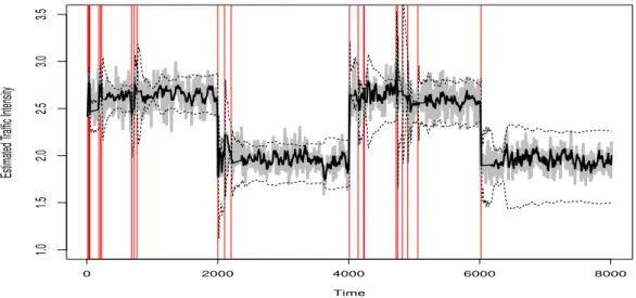
To illustrate the proposed normalized EWMA estimator and the correspond-ing control chart, we consider a particular real traffic trace collected from the In-dianapolis and Cleveland links of the Abilene backbone network. For simplicity, the trace was transformed into a time sequence of correlated arrival events as ex-pressed in 100 kilobytes per 1.5 seconds (see http://moat.nlanr.net/Images/Nvabar/ 2 MNA.html and Rolls et al. (2005) for a complete description of this data set).

The result of choosing c0 = 0.5, with the value of c being adjusted by (13), is

shown in Figure 2.

Note that in Figure 2, the lower bound (and initial value) of c is chosen to be

c0 = 0.5, which is a rule of thumb we obtained from a large number of

simula-tion trials. In addisimula-tion, the upper bound of the switching frequency is given by

p = 0.01 and the number of out-of-control signals used to estimate the ARL is

m = 3. As we can see from Figure 2, in the beginning of the first period (from time 0 to 2000) a few more out-of-control signals are generated for a relatively small value of c; while as time moves on, the value of c is automatically adjusted (increased) so that fewer out-of-control signals are generated in order to approach the preset frequency upper bound 0.01. In addition, the out-of-control signals were promptly generated right after time 2000, 4000, and 6000, where the inten-sity appears to have significant changes. For comparison purposes, we perform

a simple sensitivity analysis on the choice of the lower bound c0. The results for

choosing c0 = 0.3and c0 = 0.7are shown in Figure 3 and Figure 4, respectively.

As shown in Figure 3, a few more out-of-control signals (particularly in the

beginning) are generated by decreasing the lower bound c0 to 0.3. The result

is straightforward since the control chart becomes more sensitive on detecting small changes of the intensity. On the other hand, the control chart becomes less

sensitive on detecting small changes by increasing the lower bound c0 to 0.7. As

11 0 2000 4000 6000 8000 1.0 1.5 2.0 2.5 3.0 3.5 Time Estimated T raffic Intensity

Figure 2: An illustration of the proposed normalized EWMA estimator (black solid line) and the corresponding control limits (dashed lines) for the data (grey line) collected from the Abilene backbone network. Note that here c0 = 0.5, c is adjusted by (13), and the vertical lines represent

the times when the out-of-control signals are generated.

0 2000 4000 6000 8000 1.0 1.5 2.0 2.5 3.0 3.5 Time Estimated T raffic Intensity

Figure 3: An illustration of the proposed normalized EWMA estimator (black solid line) and the corresponding control limits (dashed lines) for the data (grey line) collected from the Abilene backbone network. Note that here c0 = 0.3, c is adjusted by (13), and the vertical lines represent

(11)

9

with various types of input traffic, say, fractional Brownian input traffic, randomly modulated compound Poisson input processes, and real traffic traces from internet. Numerical results show that the proposed method can significantly improve the QoS measures such as average delay and the 95th_{percentile of delays with a significant}

reduction on the computational/operational costs. It is worth noting that the proposed framework is novel and superior to the existing methods from the following perspectives: (i) it is purely measurement based and adaptive to any types of input traffic flow; (ii) it can be applied to any stochastic systems having similar flow analogies and control schemes (i.e., systems wherein the control can be written as a function of flow intensities); (iii) it is the first attempt to integrate the statistical online estimation, monitoring strategies, and operating costs into the control formulation of stochastic systems. We are currently investigating its performance when applied to the control problems for a variety of stochastic systems.

參考文獻

changed (recall that the control policy is designed to be responsive to instanta-neous traffic fluctuations). However, the performance of the proposed method for such systems needs to be further investigated.

4. Concluding Remarks

In this paper we propose a general framework for measuring and monitoring the flow intensities of stochastic systems. The framework employs an Exponential Weighted Moving Average (EWMA) process to estimate the traffic intensity and monitor its “significant” shifts over time. Based on the framework, an adaptive control policy can be easily developed so as to improve the performance mea-sures of interest without requiring high operating costs. To illustrate the proposed framework, we introduce a fluid control problem for a canonical queueing model. Extensive simulation results show that the proposed framework exhibits a good performance in terms of both delay and operating costs for a number of scenar-ios. It is worth noting that the proposed framework is novel and superior to the existing methods from the following perspectives: (i) it is purely measurement based and adaptive to any types of input traffic flow; (ii) it can be applied to any stochastic systems having similar flow analogies and control schemes (i.e., sys-tems wherein the control can be written as a function of flow intensities); (iii) it is the first attempt to integrate the statistical online estimation, monitoring strate-gies, and operating costs into the control formulation of stochastic systems. We are currently investigating its performance when applied to the control problems for a variety of stochastic systems.

Acknowledgement

The authors would like to thank the two anonymous reviewers for their helpful comments. This work was supported by the research grant NSC 100-2118-M-004-005.

References

[1] Aktekin T, Soyer R. Bayesian modeling of queues in call centers. The George Washington University, Technical Report TR-2010-3, 2010.

[2] Aktekin T, Soyer R. Call center arrival modeling: A Bayesian state-space ap-proach. Naval Research Logistics 2011;58: 2842. DOI: 10.1002/nav.20436.

25

[3] Armony M, Bambos N. Queueing dynamics and maximal throughput scheduling in switched processing systems. Queueing Systems: Theory and Applications 2003;44: 209-252. DOI: 10.1023/A:1024714024248.

[4] Asmussen S. Exponential families and regression in the Monte Carlo stud of queues and random walks. Annals of Statistics 1990; 18: 1851-1867. DOI: 10.1214/aos/1176347883.

[5] Baccelli F, Bremaud P. Elements of Queueing Theory (2nd edn), Springer, 2003.

[6] Bassamboo A, Randhawa RS. On the accuracy of fluid models for capacity sizing in queueing systems with impatient customers. Operations Research 2010;58: 1398-1413. DOI: 10.1287/opre.1100.0815.

[7] Bellizzi S, Bouc R. Adaptive sub-optimal parametric control for non-linear stochastic systems. Application to semi-active isolators. Probability Meth-ods in Applied Physics 1995; 451: 223-238. DOI: 10.1007/3-540-60214-3 58.

[8] Björklund E, Matinlauri I, Tierens A, Axelsson S, Forestier E, Jacobsson S, Ahlberg AJ, Kauric G, Mäntymaa P, Osnes L, Penttilä TL, Marquart H, Savolainen ER, Siitonen S, Torikka K, Mazur J, Porwit A. Quality control of flow cytometry data analysis for evaluation of minimal residual disease in bone marrow from acute leukemia patients during treatment. Journal of Pediatric Hematology/Oncology 2009;31:406-415. PMID: 19648789. [9] Le Boudec JY. Application of network calculus to guaranteed service

net-works. IEEE Transactions on Information Theory 1998; 44: 1087-1096. DOI: 10.1109/18.669170.

[10] Chan LK, Heng JC. Skewness correction ¯X and R charts for skewed distributions. Naval Research Logistics 2003; 50: 555-573. DOI: 10.1002/nav.10077.

[11] Cheng RCH, Kleijnen JPC. Improved design of queueing simulation experi-ments with highly heteroscedastic responses. Operations Research 1999;47: 762-777. DOI: 10.1287/opre.47.5.762.

(12)

10

26

[12] Cox DR. Prediction by exponentially weighted moving averages and related methods. Journal of the Royal Statistical Society. Series B 1961; 23: 414-442.

[13] Dai JG. On positive harris recurrence of multiclass queueing networks: A unified approach via fluid limit models. Annals of Applied Probability 1995; 5: 49-77. DOI: 10.1214/aoap/1177004828.

[14] Dai JG. Stability of fluid and stochastic processing networks. MaPhySto Mis-cellanea Publication, No. 9, Denmark, 1999.

[15] Dai JG, Meyn SP. Stability and convergence of moments for multi-class queueing networks via fluid limit models. IEEE Transactions on Automatic Control 1994;40: 1889-1904. DOI: 10.1109/9.471210.

[16] D’hautcourt JL. Quality control procedures for flow cytometric applications in the hematology laboratory. Hematology and Cell Therapy 1997;38: 467-470. DOI: 10.1007/s00282-996-0467-0.

[17] Duffield N. Sampling for passive internet measurement: A review. Statistical Science 2004;19: 472-498. DOI: 10.1214/088342304000000206.

[18] Egbelu PJ, Roy N. Material flow control in AGV/unit load based production lines. International Journal of Production Research 1988; 26: 81-94. DOI: 10.1080/00207548808947842.

[19] Harrison JM. The BIGSTEP approach to flow management in stochastic pro-cessing networks. In Stochastic Networks: Theory and Applications. Kelly F, Zachary S, Ziendins I (eds). Oxford University Press, 1996; 57-90. [20] Harrison JM. Heavy traffic analysis of a system with parallel servers:

asymp-totic optimality of discrete-review policies. Annals of Applied Probability 1998;8: 822-848. DOI: 10.1214/aoap/1028903452.

[21] Hayel Y, Ouarraou M, Tuffin B. Optimal measurement-based pricing for an M/M/1 queue. Networks and Spatial Economics 2007; 7: 177-195. DOI: 10.1007/s11067-006-9001-8.

[22] Hung YC, Michailidis G. Improving quality of service for switched process-ing systems. Proceedprocess-ings of 11th Intl. Workshop on Computer-Aided Mod-eling, Analysis and Design of Communication Links and Networks 2006; 46-53. DOI: 10.1109/CAMAD.2006.1649717.

(13)

11

[23] Hung YC, Michailidis G. A measurement based dynamic policy for switched processing systems. Proceedings of IEEE International Conference on Com-munications 2007; 301-306. DOI: 10.1109/ICC.2007.57.

[24] Hung YC, Michailidis G. Modeling, scheduling, and simulation of switched processing systems. ACM Transactions on Modeling and Computer Simula-tion 2008;18: Article 12. DOI: 10.1145/1371574.1371578.

[25] Hung YC, Michailidis G, Bingham DR. Developing efficient sim-ulation methodology for complex queueing networks. Proceedings of the Winter Simulation Conference 2003; 1: 512-519. DOI: 10.1109/WSC.2003.1261463.

[26] Kallitsis MG, Michailidis G, Devetsikiotis M. Measurement-based optimal resource allocation for network services with pricing differentiation. Perfor-mance Evaluation 2009;66: 505-523. DOI: 10.1016/j.peva.2009.03.003. [27] Kleijnen JPC. Regression metamodels for simulation with common random

numbers: comparison of validation tests and confidence intervals. Manage-ment Science 1992;38: 1164-1185. DOI: 10.1287/mnsc.38.8.1164.

[28] Leland WE, Taqqu MS, Willinger W, Wilson DV. On the self-similar nature of Ethernet traffic (extended version). IEEE/ACM Transactions on Network-ing 1994;2: 1-15. DOI: 10.1109/90.282603.

[29] Lowry CA, Woodall WH. A multivariate exponentially weighted moving av-erage control chart. Technometrics 1992;34: 46-53. DOI: 10.2307/1269551. [30] Meyn SP, Tweedie RL. Markov Chains and Stochastic Stability.

Springer-Verlag, 1993.

[31] Meyn SP, Tweedie RL. Criteria for stability of Markovian processes III: Foster-Lyapunov criteria for continuous time processes. Advances in Applied Probability 1993;25: 518-548. DOI: 10.2307/1427522.

[32] Montgomery DC, Mastrangelo CM. Some statistical process control meth-ods for autocorrelated data. Journal of Quality Technology 1991; 23: 179-193.

[33] Norros I. A storage model with self-similar input. Queueing Systems: Theory and Applications 1994;16: 387-396. DOI: 10.1007/BF01158964.

28

[34] Norros I. On the use of fractional Brownian motion in the theory of con-nectionless networks. IEEE Journal on Selected Areas in Communications 1995;13: 953-962. DOI: 10.1109/49.400651.

[35] Ramjee R, Crato N, Ray BK. A note on moving average forecasts of long memory processes with an application to quality control. International Jour-nal of Forecasting 2002;18: 291-297. DOI: 10.1016/S0169-2070(01)00159-5.

[36] Rolls DA, Michailidis G, Hernandez-Campos F. Queueing analysis of net-work traffic: methodology and visualization tools. Computer Netnet-works 2005;48: 447-473. DOI: 10.1016/j.comnet.2004.11.016.

[37] Ross K, Bambos N. Local search scheduling algorithms for maximal throughput in packet switches. Proceedings of IEEE INFOCOM 2004; 2: 1158-1169. DOI: 10.1109/INFCOM.2004.1357002.

[38] Ross K, Bambos N. Dynamic quality of service control in packet switch scheduling. Proceedings of IEEE International Conference on Communica-tions 2005;1: 396-401. DOI: 10.1109/ICC.2005.1494382.

[39] Seamer LC, Kuckuck F, Sklar LA. Sheath fluid control to permit stable flow in rapid mix flow cytometry. Cytometry 1999;35: 75-79.

[40] Sorte DD, Reali G. Resource allocation rules for providing performance guarantees to traffic aggregates in a DiffServ environment. Computer Com-munications 2002;25: 846-862. DOI: 10.1016/S0140-3664(01)00429-7. [41] Stolyar AL. MaxWeight scheduling in a generalized switch: state space

col-lapse and workload minimization in heavy traffic. Annals of Applied Proba-bility 2004;14: 1-53. DOI: 10.1214/aoap/1075828046.

[42] Walrand J. Introduction to Queueing Networks, Prentice Hall: Englewood Cliffs, NJ, 1988.

[43] Wasserman KM, Michailidis G, Bambos N. Optimal processor allocation to differentiated job flows. Performance Evaluation 2006; 63: 1-14. DOI: 10.1016/j.peva.2004.11.001.

(14)

12

[34] Norros I. On the use of fractional Brownian motion in the theory of

con-nectionless networks. IEEE Journal on Selected Areas in Communications 1995;13: 953-962. DOI: 10.1109/49.400651.