偏斜常態分配下損失管制圖之設計 - 政大學術集成
108
0
0
全文
(2) 謝辭 感謝 楊素芬 博士擔任我的論文指導老師,在她的指導下我的研究論文可以 順利完成。素芬老師提供我許多方向去研究、並且指導我如何解釋計算以及發現 數值分析結果的價值,在撰寫論文的過程中讓我受益良多。也感謝素芬老師對我 們的關心,時常告訴我們在未來職場如何培養正確的心態,讓我們不會膽怯。 感謝我的家人,在碩班兩年中總在我背後提供最好的支柱。感謝爸爸、媽媽 總是支持我每一項重大的決定,給我機會以及支柱去追求自己的理想。 感謝政大統研所的老師們的授教和每一次的指正,在碩班兩年讓我建立良好. 政 治 大. 的統計分析能力。感謝老師們總是這麼親和地回答我所有的統計疑問。. 立. 感謝政大統研所的同學們,感謝有你們在研究室的美好氣氛化解了寫論文和. ‧ 國. 學. 課業的壓力,提供我許多動力可以繼續努力下去。感謝我的研究夥伴 嘉煒 ,每 當研究遇上任何困難我都可以第一個找你討論。最後,謹以此文感謝我身邊所有. ‧. Nat. y. 的朋友們。. sit. 本研究承蒙行政院國家科學委員會補助,計畫編號 NSC‐102‐2118‐M‐004‐. n. al. er. io. 005‐MY2 補助,特此感謝。. Ch. engchi. 2. i n U. v. 盧尚文 謹致 一百零三年六月.
(3) ABSTRACT. In this study we construct loss-based control charts under skew-normal population. When the underlying distribution is skewed, we proposed a median loss control chart to simultaneously monitor the change of difference to process mean and target and the change of variance. An unbiased-ARL1 adjustment to the median loss chart is discussed. We also construct an average loss control chart under skew-normal population, and compare with the median loss control chart. Moreover, the EWMA or VSI charts are considered to improve the detection ability of the median loss or the. 治 政 average loss control charts. Out-of-control detection 大 ability comparison among the 立 median loss, average loss and some existed control charts for skewed population is ‧. ‧ 國. 學. io. sit. y. Nat. n. al. er. discussed.. Ch. engchi. 3. i n U. v.
(4) CONTENTS Chapter 1.. Introduction ............................................................................................... 2. 1.1 Research Motivation .......................................................................................... 2 1.2 Literature Review .............................................................................................. 2 1.3 Research Method ............................................................................................... 5 Chapter 2. The Sampling Distribution of the Median Loss for Skew Normal Population ............................................................................................................... 6 2.1 Derivation the Distribution of the Sample Median Loss ................................... 6 2.1.1 The probability density and the distribution function of the skew-normal random variable ........................................................................................ 6 2.1.2 The pdf and cdf of Taguchi Loss ............................................................... 8. 政 治 大. 2.1.3 The pdf and cdf of the Median Loss ......................................................... 9 2.2 Cumulative Distribution Function derivation of the Sample Median Loss ..... 10. 立. Chapter 3. Constructions of the Median Loss, EWMA and Optimal VSI Median Loss. ‧ 國. 學. Control Charts ....................................................................................................... 13 3.1 Construction of the Median Loss Control Chart.............................................. 13 3.1.1 Control limits of the Median Loss chart ................................................. 13. ‧. 3.1.2 Performance Measurement of the Median Loss chart ............................ 16 3.2. An EWMA Median Loss Chart....................................................................... 44. y. Nat. sit. 3.2.1 Construction of the EWMA-ML Chart ................................................... 44. io. er. 3.2.2 The out-of-control detection Performance Measurement of the EWMA-ML Chart................................................................................... 47. al. n. v i n C EWMA Median Loss Median Loss and the h e n g c h i U Charts ................................ 49. 3.2.3 The Out-of-Control Detection Performance Comparison between the. 3.3. An Optimal Variable Sampling Interval Median Loss Chart .......................... 51 3.3.1 Construction of the Optimal VSI Median Loss Chart ............................. 52 3.3.2 Performance Measurement of the VSI Median Loss Chart .................... 53 3.3.3 ATS1s Comparison among the Median Loss Chart, specified VSI Median Loss Chart and the Optimal VSI Median Loss Chart ............................. 56 Chapter 4. Constructions of the AL, EWMA-AL, Optimal VSI-AL Control Charts under Skew normal distribution ............................................................................ 60 4.1 Construction of the Average Loss Chart .......................................................... 61 4.1.1 Approximate Distribution of Average Loss by Using Edgeworth Expansion Method .................................................................................. 61 4.1.2 Control Limits of the Average Loss Chart .............................................. 65 4.1.3 Out-of-Control Detection Performance Measurement of the AL Chart .. 68 II.
(5) 4.2. An EWMA Average Loss Chart ...................................................................... 73 4.2.1 Construction of the EWMA-AL Chart .................................................... 73 4.2.2 Out-of-Control Detection Performance Measurement of the EWMA-AL Chart ....................................................................................................... 74 4.2.3 Out-of-Control Detection Performance Comparison among the AL and the EWMA-AL Chart ............................................................................. 75 4.3. An Optimal Variable Sampling Interval Average Loss Chart ......................... 77 4.3.1 Construction of the Optimal VSI Average Loss Chart ............................ 77 4.3.2 Out-of-control Detection Performance Measurement of the Optimal VSI Average Loss Chart ................................................................................. 79 4.3.3 ATS1s Comparison among the AL Chart, specified VSI-AL Chart and the Optimal VSI-AL Chart ........................................................................... 79. 政 治 大. Chapter 5. ATS1 Comparison among all Proposed Loss Control Charts and Other Existed Control Charts .......................................................................................... 84. 立. 5.1 Introduction of Some Existed Control Charts ................................................. 84. ‧ 國. 學. 5.2 ATS1 Comparison among all Proposed Loss Control Charts and Other Existed Control Charts ........................................................................................................ 87 Chapter 6. Conclusions and Future Study.................................................................... 98. ‧. Reference ..................................................................................................................... 99. n. er. io. sit. y. Nat. al. Ch. engchi. III. i n U. v.
(6) LIST OF TABLES Table 2-1 The skewness of the skew-normal distribution ............................................. 7 Table 3-1.1 Control limits of the ML Chart ................................................................ 14 Table 3-1.1 (Continued) .............................................................................................. 15 Table 3-1.2 Control limits of ML Chart ...................................................................... 15 Table 3-2.1 ARL1 of ML Chart ( 0.0027 , n 5 , 0 0 , 0 1 , b 500, 0, 500 ) ................................. 18 Table 3-2.1 (Continued) .............................................................................................. 19 Table 3-2.1 (Continued) .............................................................................................. 20 Table 3-2.2 ARL1 of ML Chart ( 0.0027 , n 5 , 0 0 , 0 1 , b 2, 0, 2 ) ......................................... 21. 政 治 大 Table 3-14 Control Limits 立 of the Unbiased-ARL ML chart under. Table 3-3 Response table for ARL1 of ML chart ...................................................... 28 1. b 0 and 3 0. .............................................................................................................................. 34. ‧ 國. 學. Table 3-15 Values of ( L1 , L2 ) and the combination of 1 and 2 such that ARL1 < ARL0 ....................................................................................................... 36. ‧. Table 3-16 The Feasible Values of ( L1, L2 ) for Various Combinations of n, 1 , 2 , 3 and b such that ARL1 < ARL0 ..................................................................... 38. Nat. sit. y. Table 3-16 (Continued) ............................................................................................... 39. er. io. Table 3-17 The ARL1 comparison between ARL1-biased and unbiased ML charts ( n 5 , 0 0 , 0 1 , 0.0027 ) .................................................................... 42. al. n. v i n Ch .............................................................................................................................. 43 engchi U Table 3-19 Control limits of the EWMA-ML chart Table 3-18 The Comparison Among the Three ARL-unbiased and -unbiased Methods.. ( n 5 , 0 0 , 0 1 , ARL0 370.4 and 3 1 ) ........................................... 47 Table 3-20.1 ARL1s of the EWMA-ML chart ( 0.05 ) and the ML chart .............. 50 Table 3-20.2 ARL1s of the EWMA-ML chart ( 0.05 ) and the ML chart .............. 51 Table 3-20 ATS1s of optimal VSI-ML chart, specified VSI-ML chart and the ML chart .............................................................................................................................. 57 Table 3-20 (Continued) ............................................................................................... 58 Table 3-20 (Continued) ............................................................................................... 59 Table 4-1 The Hermite polynomial ............................................................................. 62 Table 4-2 The cumulants of L ( X T )2 ................................................................. 62 Table 4-3 P-value of the Pearson 2 goodness-of-fit test for Edgeworth expansion .............................................................................................................................. 64 Table 4-4.1 Control limits of the AL Chart ................................................................. 66 IV.
(7) Table 4-4.1 (Continued) .............................................................................................. 67 Table 4-4.2 Control limits of AL Chart ....................................................................... 68 Table 4-5.1 The ARL1 of the AL chart ........................................................................ 69 Table 4-5.1 (Continued) .............................................................................................. 70 Table 4-5.2 The ARL1 of the AL chart ........................................................................ 71 Table 4-6 The response table for ARL1 of the AL chart ........................................... 72 Table 4-7 The control limits of the EWMA-AL chart ( n 5 , ARL0 370.4 ) ......... 74 Table 4-8.1 The ARL1s comparison of the EWMA-AL and the AL charts ................. 76 Table 4-8.2 The ARL1s comparison of the EWMA-AL and the AL charts ................. 77 Table 4-10 ATS1s of optimal VSI-AL chart, specified VSI-AL chart and the AL chart .............................................................................................................................. 81. 政 治 大. Table 4-10 (Continued) ............................................................................................... 82 Table 4-10 (Continued) ............................................................................................... 83. 立. Table 5-1 Chart parameters for WV Method ............................................................... 85. ‧ 國. 學. Table 5-2 Chart parameters for SC Method ................................................................ 87 Table 5-3 The ATS1s comparison among the 8 methods when b 500 and 3 0. ‧. .............................................................................................................................. 88 Table 5-4 The ATS1s comparison among the 8 charts when b 0 and 3 0 ........ 90 Table 5-5 The ATS1s among the 8 charts when b 500 and 3 0 ....................... 91. y. Nat. Table 5-6 The ATS1s comparison among the 8 charts when b 500 and 3 1 .. 92. sit. Table 5-7 The ATS1s comparison among the 8 methods when b 0 and 3 1 .... 93. n. al. er. io. Table 5-8 The ATS1s among the 8 charts when b 500 and 3 1 ....................... 94. i n U. v. Table 5-9 The performance comparison among the eight charts ................................ 97. Ch. engchi. V.
(8) LIST OF FIGURES Fig. 2-1 The pdfs of skew-normal distribution .............................................................. 7 Fig. 3-1 b 500 , 2 =1 ........................................................................................... 22 Fig. 3-2 b 0 , 2 =1 ................................................................................................. 22 Fig. 3-3 b 500 , 2 =1 ............................................................................................. 23 Fig. 3-4 b 500 , 1 =0 ............................................................................................ 23 Fig. 3-5 b 0 , 1 =0 .................................................................................................. 24 Fig. 3-6 b 500 , 1 =0 .............................................................................................. 24 Fig. 3-7 b 500 , 2 3 ......................................................................................... 25 Fig. 3-8 b 0 , 2 =3 ................................................................................................. 25 Fig. 3-9 b 500 , 2 3 ........................................................................................... 25 Fig. 3-10 b 500 , 1 =3 .......................................................................................... 27 Fig. 3-11 b 0 , 1 =3 ................................................................................................ 27. 政 治 大. Fig. 3-12 b 500 , 1 =3 ............................................................................................ 27. 立. Fig. 3-13 Response diagram for ARL1 of ML chart .................................................. 28. ‧ 國. 學. Fig. 3-14 Biased ARL of the ML chart ........................................................................ 30. ‧. Fig. 3-15 The ARL of ARL1-unbiased ML chart ( 0.0027 , 0 0 , 0 1 , 3 0 and b 0 ) ......................................... 35. Nat. Fig. 4-1 The approximated cdf of AL by Edgeworth expansion. y. Fig. 3-17 A visualization of the VSI-ML chart ............................................................ 52. er. io. sit. ( m 50000 for the simulated cdf of AL) ........................................................... 65. al. Fig. 4-2 Response diagram for ARL1 of the AL chart ............................................... 72. n. v i n VSI-AL ........................................................... 78 Fig. 4-3 The visualization of theC h e nchart gchi U Fig. 5-1 The response diagram of the ATS1 s for the eight charts when b 500 and 3 0 ............................................................................... 89 Fig. 5-2 The response diagram of the ATS1 s for the eight charts when b 0 and 3 0 ..................................................................................... 90 Fig. 5-3 The response diagram of the ATS1 s for the eight charts when b 500 and 3 0 ................................................................................. 91 Fig. 5-4 The response diagram of the ATS1 s for the eight charts when b 500 and 3 1 ............................................................................... 92 VI.
(9) Fig. 5-5 The response diagram of the ATS1 for the eight methods when b 0 and 3 1 ..................................................................................... 93 Fig. 5-6 The response diagram of the ATS1 s for the eight charts when b 500 and 3 1 ................................................................................. 94. 立. 政 治 大. ‧. ‧ 國. 學. n. er. io. sit. y. Nat. al. Ch. engchi. VII. i n U. v.
(10) Chapter 1.. Introduction. 1.1 Research Motivation Sample median is a statistic better than the sample average to measure the population center when the underlying distribution is skewed, since its robustness to the outliers, see Graham, et al. (2010). When we are dealing with process control, in reality the distribution of the quality characteristic may be skewed, therefore it is reasonable to use median type control charts for process monitoring.. 政 治 大. The Taguchi loss function, which is an important indicator in many industries, is. 立. a useful tool to measure the loss caused by deviation of the quality characteristic from. ‧ 國. 學. its target value. The expectation of Taguchi loss consists of the population variance and the squared difference between population mean and the target value. Therefore it. ‧. can be used for process control for change of variance and the difference between. y. Nat. n. er. io. al. sit. process mean and the target value.. i n U. v. So we consider using median loss (ML) statistic to construct several ML related. Ch. engchi. control charts to monitor the change of process mean and variance simultaneously, assuming that the underlying distribution of the quality characteristic is skewed. We also construct sample average loss (AL) related control charts in order to compare the performance with those of the ML type control charts, and we will discuss the advantages and disadvantages of those proposed control charts, respectively.. 1.2 Literature Review Control charts are widely used in monitoring and improving a process. Control charts based on normal assumption of the quality characteristics have been widely 2.
(11) studied. When the distribution of the quality characteristic is skewed, the use of those control charts may be misleading. Bai and Choi (1995) proposed a weighted variance (WV) X and R charts using the in-control probability that X smaller than its population mean to adjust the control limits of Shewhart type X and R charts when the distribution is skewed. Chan and Cui (2007) proposed a skewness correction (SC) method for constructing X and R chart taking into consideration the degree of skewness of the process distribution, with no assumptions on the distribution. They found that when the process distribution is Weibull, lognormal, Burr or binomial. 政 治 大 to its theoretical value than the WV and Shewhart type charts. 立. distribution, simulation shows that the SC control chart has real false alarm rate closer. ‧ 國. 學. Graham, Human & Chakraborti (2010) proposed a nonparametric median type. ‧. control chart. The monitoring statistic for each sample is the count of Xi less than the pooled median. The pooled median is an estimator of population median calculated. y. Nat. er. io. sit. from in-control samples during Phase I. They found that the median chart has in-control robustness to the outliers while X chart does not when the underlying. al. n. v i n distribution is skewed. They also right-skewed distributions the median Cfound h e nthatgfor h c i U chart may perform better for positive shifts of process location. However, the median chart has poorer detection ability for shift of process location than the X chart when the distribution is symmetric. Yang, Pai, & Wang (2010) compare some median type. ~ ~ ~ control charts, such as median ( X ) chart, EWMA- X chart and the CUSUM- X chart, to those of the X type control charts under normality assumption. They also found that the median control charts are robust to outliers while mean control charts are very sensitive to outliers.To measure the performance of a control chart, average run length (ARL) is widely used. ARL is unbiased for symmetrically distributed 3.
(12) monitoring statistic. However, the ARL1 of the control chart may exceed ARL0 when the underlying distribution is skewed. Pignatiello, Acosta, and Rao (1995) defined the concept of an ARL-unbiased control chart. That is, the control chart is said to be ARL-unbiased if its ARL curve achieves its maximum when the process parameter is equal to its in-control value. Sven and Manuel (2013) proposed an ARL-unbiased S 2 chart and an EWMA- S 2 chart to monitor process dispersion. Pascual (2013) proposed combined individual and moving range charts with ARL-unbiasedness for monitoring changes in either the Weibull scale or shape parameter.. 治 政 The Taguchi loss function is developed by Taguchi 大(1986) to measure the loss 立 caused by deviation of the quality characteristic from its target value. Yang (2013a) ‧ 國. 學. proposed an average loss chart to simultaneously monitor the process mean and the. ‧. variability. Yang (2013b) proposed an EWMA average loss chart with variable sampling intervals (VSI) to monitor the changes in the difference of process mean and. y. Nat. er. io. sit. target and process variance. The out-of-control process diagnosis approach is also discussed. However, those charts were based on the normality assumption of the. al. n. v i n quality characteristic, and a lossCcontrol chart under skewed distribution has yet been hengchi U discussed.. A control chart with VSI is a control technique that can reduce the out-of-control detection time when the process going out-of-control. The properties of the VSI X chart were first studied by Reynolds et al. (1988). Their work has been inspired for several other papers, for example Costa (1995) proposed a X chart with Variable Sample Sizes and Sampling Intervals (VSSI). Yang (2013b) proposed an optimal VSI-EWMA Average Loss Chart which minimizes the average time to signal when. 4.
(13) process going out-of-control. Some other adaptive control schemes related literatures may refer to Yang (2013b).. 1.3 Research Method In this study we propose some median loss (ML) type control charts, assuming that the distribution of the quality characteristic (X) follows skew-normal distribution. And we consider the distribution to be right-skewed, symmetric or left-skewed.. For fixed sampling interval (FSI) of the chart, we propose ML and EWMA-ML. 治 政 charts respectively to detect the process change of mean 大and variance simultaneously 立 under skew-normal assumption. However, if the sampling intervals of the chart can be ‧ 國. 學. variable, an optimal VSI-ML chart is proposed to save the detection time when. ‧. process going out-of-control. We also propose some average loss (AL) type control charts, including AL, EWMA-AL,optimal VSI-AL charts to compare the performance. y. Nat. n. al. er. io. sit. with ML type charts.. Ch. engchi. 5. i n U. v.
(14) Chapter 2. The Sampling Distribution of the Median Loss for Skew Normal Population The control charts we proposed in this study are all assumed that the quality characteristic X follows skew-normal distribution. The skew normal distribution is first introduced by O’Hagan and Leonard (1976). Azzalini (1985, 1986) discussed some properties about this distribution.. 2.1 Derivation the Distribution of the Sample Median Loss. 政 治 大. 2.1.1 The probability density and the distribution function of the skew-normal random variable. 立. ‧ 國. 學. Denote random variable X has skew-normal distribution with location parameter. 0 ( , ) , scale parameter a0 (0, ) and shape parameter b ( , ) . That. ‧. is, X ~ SN (0 , a0 , b) . From Azzalini (1985), the probability density function (pdf). er. io. sit. y. Nat. of X is. aa2l ( x a )(b x a ) , xiv(, ) n Ch U engchi. f X ( x) . n. 0. 0. 0. 0. (2-1). 0. where () and () are respectively the pdf and cumulated distribution function (cdf) of the standard normal distribution. In (2-1), we know that if b 0 the skew-normal distribution will reduce to normal with mean 0 and standard deviation. a0 .. The skewness of the skew-normal distribution is uniquely determined by the shape parameter b , which is in the form of. 6.
(15) k3 ( X ) . 2 ( 4 )b 3. (2-2). ( 2)b . 2 3/ 2. From (2-2) it shows that the skewness is bounded by (0.9953, 0.9953) . Furthermore, when b , the skew-normal tends to the half-normal distribution. Table 2-1 gives the values of b and the corresponding skewness of the distribution.. Table 2-1 The skewness of the skew-normal distribution b. 政 治 大 -0.9953. -5. -0.851. -2. -0.4538. 0. 0. 2. 0.4538. 5. 0.851. 500. 0.9953. ‧. -500. 學. ‧ 國. 立. K3(X). y. Nat. sit. Figure 2-1 shows the pdfs of skew-normal distribution with 0 0 , a0 1 , and. n. al. er. io. with b 500, 2, 0, 2, 500 respectively.. Ch. engchi. i n U. v. Fig. 2-1 The pdfs of skew-normal distribution. 7.
(16) The cdf of the skew normal random variable X is. x 0 1 b FX ( x ) a0 0. exp{. 1 x 0 2 ( ) (1 y 2 )} 2 a0 dy , 1 y2. x (, ) .. (2-3). The expectation ( 0 ) and variance ( 02 ) of X are. 0 0 a0. b. 2. 1 b2. . . , 02 a02 1 . 2b2 . (1 b2 ) . So if we know 0 , 02 and shape b , we can obtain. 政 治 大 2b , a. 立 (1 b ) 2b. 0 0 . 0. 2. 2. 0. .. ‧ 國. 學. 2b 2 1 (1 b2 ). ‧. We are proceed to derive the distribution of sample median loss, when the process is in-control and X follows SN (0 , a0 , b) .. sit. y. Nat. n. al. er. io. 2.1.2 The pdf and cdf of Taguchi Loss. Ch. The Taguchi loss function is defined as. engchi. v i n L k( X T ) U. 2. . Without loss of. generality, we set k 1 . When X follows skew-normal distribution, The cdf of ( X T )2 can be found by. F( X T )2 (t ) P(( X T ) 2 t ) P( t X T t ) FX ( t T ) FX ( t T ) t T 0 T t 0 1 a0 a0 . . b. e. 1 T t 0 2 ( ) (1 y 2 ) 2 a0. 1 t T 0 2 ( ) (1 y 2 ) 2 a0. e 1 y2. 0. where t 0 .. 8. dy ,. (2-4).
(17) The pdf of ( X T )2 may be derived by. f ( X T )2 (t ) . . 1 a0. . . d 1 F( X T )2 (t ) f X ( t T ) f X ( t T ) dt 2 t. t T 0 t T 0 t T 0 t T 0 . ) ( b ) ( ) ( b ) ( a0 a0 a0 a0 t . (2-5). 2.1.3 The pdf and cdf of the Median Loss Let X 1 , X 2 , ..., X n be an independent and identically distributed (i.i.d) sample from. 政 治 大 n is odd, the sample median loss is ML ( X T ) . Follow the inference of order 立. th SN ( , a, b) . Then the i sample loss is Li ( X i T ) 2 , i=1,…,n . When sample size 2 n 1 ) 2. 學. ‧ 國. (. statistic, for example see Jean and Subhabrata (2011), the pdf of ML is. . . ‧. f ML (t ) . (2-6). er. io. sit. y. Nat. n 1 n! F( X T )2 (t )[1 F( X T )2 (t )] 2 f ( X T )2 (t ) , n 1 2 [( )! ] 2. t 0 , where F( X T )2 () and f ( X T ) () are in forms of (2-4) and (2-5). Otherwise. n. al. 2. Ch. i n U. v. when n is even, the sample median loss is ML2 L( n / 2) L( n / 21) / 2 , the pdf of ML2. engchi. is. . 1 1 2 n! 2 2 f ML2 (t ) [ F [ 1 F f ( X T )2 (2t v ) f ( X T )2 (v )dv 2 ( 2t v )] 2 ( v )] ( X T ) ( X T ) n [( 1)! ]2 t 2 n. n. 9. (2-7).
(18) 2.2 Cumulative Distribution Function derivation of the Sample Median Loss In this section we proceed to derivate the cdf of median loss. When sample size is odd, the sample median loss is ML ( X T ) 2n1 , then we have (. t. FML (t ) f M (u)du 0. . . n! n 1 2 [( )! ] 2. . F. ( X T ) 2. ). n 1 n 1 n! 2 2 F ( u ) [ 1 F ( u )] f ( X T )2 (u)du ( X T ) 2 n 1 2 0 ( X T )2 [( )! ] 2 t. (t ). F( X T )2 (u). 0. n 1 1 2. n! n 1 n 1 B( F( X T )2 (t ), , ) n 1 2 2 2 [( )! ] 2. 立. [1 F( X T )2 (u )]. n 1 1 2. d ( F( X T )2 (u)). 政 治 大. 1 n! t T 0 t T 0 t T 0 t T 0 B ( ) ( b ) ( ) ( b ) , n 1 2 a0 a0 a0 a0 [( )! ] a0 t 2 n 1 n 1 , , 2 2 . t 0,. ‧. ‧ 國. 學. . 2. Nat. y. (2-8). x. sit. where B( x, a, b) t a 1 (1 t )b1 dt is the incomplete beta function. 0. io. er. When sample size is even, the sample median loss denote ML2 L( n / 2) L( n / 21) / 2 ,. n. al. the cdf of ML2 t. i n C is derived by the following h e n gprocedure chi U. FML2 (t ) f ML2 (u )du 0. . 2 n! n [( 1)! ]2 2. t . n. 1. v. n. 1. F( X T )2 (2u v) 2 [1 F( X T )2 (v)]2 f( X T )2 (2u v) f( X T )2 (v)dvdu 0 u. t v n n 1 1 2 n! 2 2 F [ 1 F f ( X T )2 (2u v ) f ( X T )2 (v )dudv 2 ( 2u v ) 2 ( v )] ( X T ) ( X T ) n [( 1)! ]2 0 0 2. n n 1 1 F( X T )2 (2u v ) 2 [1 F( X T )2 (v )] 2 f ( X T )2 (2u v ) f ( X T )2 (v )dudv , t 0 t. 10. (2-9).
(19) where the first part of (2-9) can be rearranged as follows t v. n. n. 1. 1. F( X T )2 (2u v) 2 [1 F( X T )2 (v)]2 f( X T )2 (2u v) f( X T )2 (v)dudv 0 0. t. [1 F( X T )2 (v )]. n 1 2. n 1 v f ( X T )2 (v ) F( X T )2 (2u v ) 2 f ( X T )2 (2u v )du dv 0 . n 1 2. n 1 1 F( X T )2 ( v ) f ( X T )2 (v ) F( X T )2 (2u v ) 2 d ( F( X T )2 (2u v )) dv F ( v) 2 ( X T ) 2 . 0. t. [1 F( X T )2 (v )] 0. t n n n 1 1 [1 F( X T )2 (v )] 2 f ( X T )2 (v ) F( X T )2 (v ) 2 F( X T )2 ( v ) 2 dv 0 n . 政 治 大. 立. n. n. ‧. ‧ 國. 學. 11 1 1 F 2 (t ) 1 n n ( X T ) F( X T )2 (v ) 2 [1 F( X T )2 (v )] 2 d ( F( X T )2 (v )) B( F( X T )2 (t ), 1, ) 0 n n 2 2. (2u v ). [1 F( X T )2 (v )]. io. n. al. f ( X T )2 (2u v ) f ( X T )2 (v )dudv. sit. ( X T )2. t 0. n 1 2. er. F. n 1 2. Nat. t. y. The second part of (2-9) can be rearranged as. v. n n 1 1 t [1 F( X T )2 (v )] 2 f ( X T )2 (v ) F( X T )2 (2u v ) 2 f ( X T )2 (2u v )du dv t 0 . Ch. engchi. i n U. n n 1 1 1 F 2 ( 2 t v ) [1 F( X T )2 (v )] 2 f ( X T )2 (v ) ( X T ) F( X T )2 (2u v ) 2 d ( F( X T )2 (2u v )) dv F ( v) 2 ( X T ) 2 t. n n n 1 1 [1 F( X T )2 (v )] 2 f ( X T )2 (v ) F( X T )2 (2t v ) 2 F( X T )2 ( v ) 2 dv t n . . n. n. 1 1 F( X T )2 (2t v ) 2 [1 F( X T )2 (v )] 2 f ( X T )2 (v )dv nt. 2t. n. n. 1 1 F( X T )2 (2t v ) 2 [1 F( X T )2 (v )] 2 f ( X T )2 (v )dv nt. 11. (since F( X T )2 ( v) 0 for v 0 ).
(20) Finally, combine the two parts in above equations the cdf of ML2 is. FML2 (t ) . 2t n n 1 2 (n 1)! n n 2 2 B ( F ( t ), 1 , ) F ( 2 t v ) [ 1 F ( v )] f ( X T )2 (v )dv ,(2-10) 2 2 2 ( X T ) ( X T ) ( X T ) n 2 2 t [( 1)! ]2 2. where F( X T )2 () and f ( X T )2 () are in forms of (2-4) and (2-5).. 立. 政 治 大. ‧. ‧ 國. 學. n. er. io. sit. y. Nat. al. Ch. engchi. 12. i n U. v.
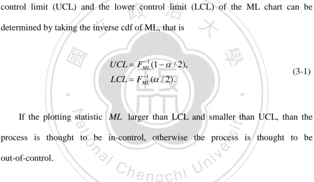
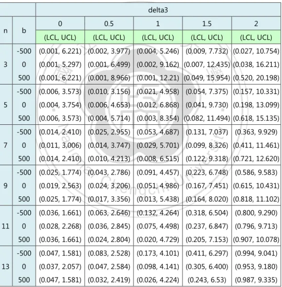
(21) Chapter 3. Constructions of the Median Loss, EWMA and Optimal VSI Median Loss Control Charts 3.1 Construction of the Median Loss Control Chart 3.1.1 Control limits of the Median Loss chart. Since the statistic of sample median loss depends on sample size be odd or even, for simplicity we only consider odd sample size in this study. From (2-8), we may construct the Median Loss (ML) control chart with false alarm rate . The upper. 政 治 大 determined by taking the inverse cdf of ML, that is 立. 學. ‧ 國. control limit (UCL) and the lower control limit (LCL) of the ML chart can be. 1 UCL FML (1 / 2),. (3-1). ‧. 1 LCL FML ( / 2).. y. Nat. sit. If the plotting statistic ML larger than LCL and smaller than UCL, than the. al. n. out-of-control.. er. io. process is thought to be in-control, otherwise the process is thought to be. Ch. engchi. i n U. v. Let 3 denote the dispersion parameter which satisfies 0 T 3 0 . Without loss of generality we set 3 0 . Table 3-1.1 gives the control limits of ML chart for various combinations of n 3, 5, ..., 51 , 3 0, 0.5, ..., 2 and b 500, 0, 500 under 0.0027 , 0 0 and 0 1 .. Table 3-1.2 gives the control limits of ML chart for various combinations of n 5, 10, 20 , 3 0, 1, 2 and b 2, 0, 2 under 0.0027 , 0 0 and 0 1 .. 13.
(22) From both Table 3-1.1 and Table 3-1.2 we can see that the width of the control limits are narrower when sample size increases. Under the cases 3 0 , the ML chart control limits when b 500 (2) are the same with b 500 ( 2 ). When 3 is greater than zero, the control limits when right-skewed are the widest, and left-skewed are the narrowest.. Table 3-1.1 Control limits of the ML Chart delta3. 13. 2. (LCL, UCL). (LCL, UCL). (LCL, UCL). (LCL, UCL). (LCL, UCL). 立. -500. (0.001, 6.221) (0.002, 3.977) (0.004, 5.246) (0.009, 7.732) (0.027, 10.754). 0. (0.001, 5.297) (0.001, 6.499) (0.002, 9.162) (0.007, 12.435) (0.038, 16.211). 500. (0.001, 6.221) (0.001, 8.966) (0.001, 12.21) (0.049, 15.954) (0.520, 20.198). -500. (0.006, 3.573) (0.010, 3.156) (0.021, 4.958) (0.054, 7.375) (0.157, 10.331). 0. (0.004, 3.754) (0.006, 4.653) (0.012, 6.868) (0.041, 9.730) (0.198, 13.099). 500. (0.006, 3.573) (0.004, 5.714) (0.003, 8.354) (0.082, 11.494) (0.618, 15.135). -500. (0.014, 2.410) (0.025, 2.955) (0.053, 4.687) (0.131, 7.037) (0.363, 9.929). 0. (0.011, 3.006) (0.014, 3.747) (0.029, 5.701) (0.099, 8.326) (0.411, 11.461). 500. (0.014, 2.410) (0.010, 4.213) (0.008, 6.515) (0.122, 9.318) (0.721, 12.620). -500. (0.025, 1.774) (0.043, 2.786) (0.091, 4.457) (0.223, 6.748) (0.586, 9.583). 0. y. sit. er. al. v i n C 3.206) (0.051, 4.986)U(0.167, 7.451) (0.024, h engchi. n. 11. 1.5. io. 9. 1. Nat. 7. 0.5. ‧. 5. 政 治 大. 0. 學. 3. b. ‧ 國. n. (0.019, 2.563). (0.615, 10.431). 500. (0.025, 1.774) (0.017, 3.356) (0.013, 5.438) (0.164, 8.020) (0.818, 11.102). -500. (0.036, 1.661) (0.063, 2.646) (0.132, 4.264) (0.318, 6.504) (0.800, 9.290). 0. (0.028, 2.268) (0.036, 2.845) (0.075, 4.498) (0.237, 6.847) (0.796, 9.713). 500. (0.036, 1.661) (0.024, 2.804) (0.020, 4.729) (0.205, 7.153) (0.907, 10.078). -500. (0.047, 1.581) (0.083, 2.528) (0.173, 4.101) (0.411, 6.297) (0.994, 9.041). 0. (0.037, 2.057) (0.047, 2.584) (0.098, 4.141) (0.305, 6.400) (0.953, 9.180). 500. (0.047, 1.581) (0.032, 2.419) (0.026, 4.224). 14. (0.243, 6.53). (0.987, 9.335).
(23) Table 3-1.1 (Continued) delta3 2. (LCL, UCL). (LCL, UCL). (LCL, UCL). (LCL, UCL). (LCL, UCL). -500. (0.058, 1.514) (0.102, 2.429) (0.213, 3.962) (0.498, 6.120) (1.168, 8.828). 0. (0.045, 1.897) (0.058, 2.387) (0.121, 3.867) (0.369, 6.054) (1.090, 8.764). 500. (0.058, 1.514) (0.039, 2.135) (0.032, 3.846) (0.280, 6.058) (1.059, 8.769). -500. (0.079, 1.408) (0.139, 2.270) (0.286, 3.739) (0.655, 5.832) (1.462, 8.479). 0. (0.062, 1.671) (0.079, 2.107) (0.164, 3.471) (0.482, 5.549) (1.317, 8.154). 500. (0.079, 1.408) (0.053, 1.744) (0.043, 3.315) (0.346, 5.386) (1.185, 7.956). -500. (0.088, 1.365) (0.156, 2.206) (0.320, 3.647) (0.725, 5.714) (1.587, 8.336). 0. (0.069, 1.587) (0.089, 2.003) (0.184, 3.322) (0.533, 5.358) (1.412, 7.921). 政 治 大. 500. (0.088, 1.365). (0.06, 1.604). -500. (0.106, 1.293) (0.186, 2.098) (0.381, 3.493) (0.848, 5.514) (1.802, 8.092). 0. (0.084, 1.457) (0.107, 1.841) (0.221, 3.087) (0.622, 5.052) (1.574, 7.548). 500. (0.106, 1.293) (0.072, 1.389) (0.058, 2.818) (0.430, 4.747) (1.336, 7.175). -500. (0.122, 1.236) (0.214, 2.012) (0.435, 3.368) (0.954, 5.350) (1.981, 7.892). 0. (0.096, 1.359) (0.123, 1.719) (0.254, 2.909) (0.699, 4.817) (1.708, 7.260). 500. (0.122, 1.236) (0.083, 1.233) (0.067, 2.593) (0.478, 4.454) (1.419, 6.814). 立. (0.049, 3.120) (0.376, 5.137) (1.239, 7.653). ‧. 29. 1.5. 學. 25. 1. Nat. y. 21. 0.5. io. sit. 19. 0. Table 3-1.2 Control limits of ML Chart. n. al. er. 15. b. ‧ 國. n. n. 5. 11. 21. Ch. v. 1. 2. (LCL, UCL). (LCL, UCL). (LCL, UCL). -2. (0.004, 3.707). (0.016, 6.190). (0.176, 12.086). 0. (0.004, 3.754). (0.012, 6.868). (0.198, 13.099). 2. (0.004, 3.707). (0.009, 7.546). (0.283, 14.040). -2. (0.027, 2.192). (0.102, 4.374). (0.814, 9.463). 0. (0.028, 2.268). (0.075, 4.498). (0.796, 9.713). 2. (0.027, 2.192). (0.054, 4.542). (0.855, 9.802). -2. (0.069, 1.534). (0.248, 3.402). (1.520, 7.976). 0. (0.069, 1.587). (0.184, 3.322). (1.412, 7.921). 2. (0.069, 1.534). (0.136, 3.168). (1.383, 7.721). b. 0. e n gdelta3 chi. i n U. 15.
(24) 3.1.2 Performance Measurement of the Median Loss chart 3.1.2.1 Biased ARL. In this section, we use Average Run Length (ARL) to measure the performance of ML chart. ARL is the average number of samples before the control chart produces a signal, which is the most popular performance measure for a control chart. The in-control process ARL (ARL0) is always fixed in a request level, for example 370.4, while the out-of-control process ARL (ARL1) is as small as better.. The ARL0 for the ML chart is. 立. 政 治 大. ‧ 國. 1. . ,. (3-2). 學. ARL0 . ‧. where P( LCL ML UCL | in control ML) is the false alarm rate.. y. Nat. er. io. sit. We are going to derive the out-of-control distribution of the sample median loss to calculate ARL1 values of the ML chart. Suppose that X * is the quality. n. al. characteristic when process. i n going out-of-control, and C hengchi U. v. X * ~ SN ( * , a * , b) with. expectation 1 0 1 0 , 1 0 , and standard deviation 1 2 0 , 2 1 , then we have:. * 0 1 0 . 2b 2 0 (1 b2 ) 2b2. * , a . 16. 2 0 2b2 1 (1 b2 ). ..
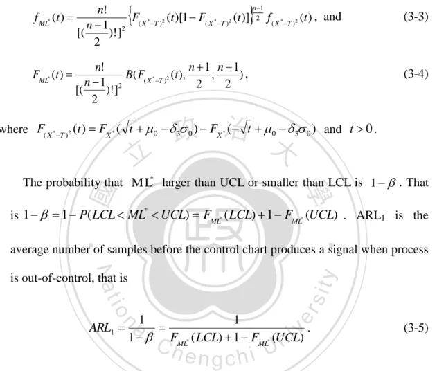
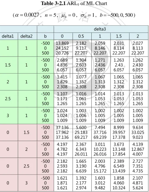
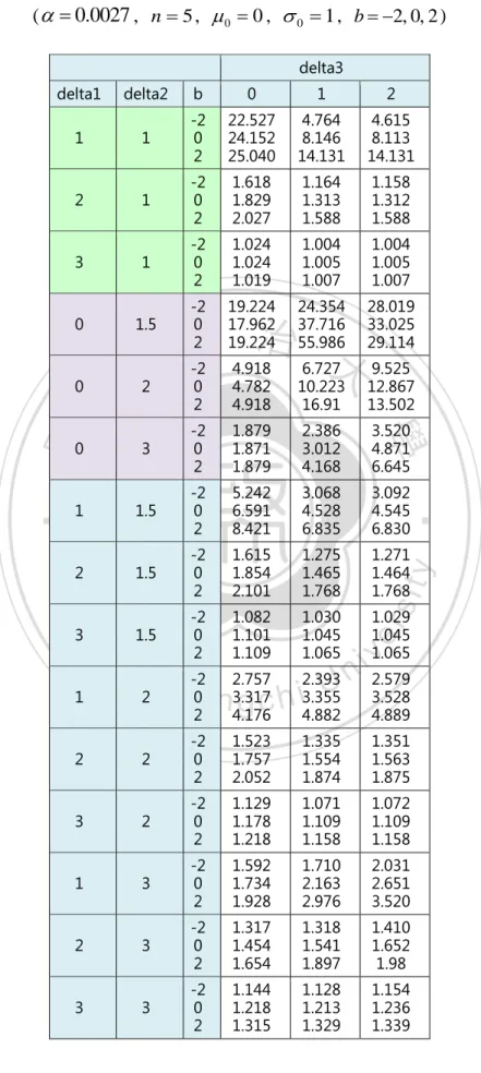
(25) When sample size is odd, the out-of-control median loss is ML* ( X * T ) 2n1 . (. 2. ). Following the same proving procedure in section 3.1 and 3.2, we can obtain the pdf and cdf of ML* as. f ML* (t ) . FML* (t ) . . . n 1 n! F( X * T )2 (t )[1 F( X * T )2 (t )] 2 f ( X * T )2 (t ) , and n 1 2 [( )! ] 2. n! n 1 n 1 B( F( X * T )2 (t ), , ), n 1 2 2 2 [( )! ] 2. (3-3). (3-4). 政 治 大. where F( X * T )2 (t ) FX * ( t 0 3 0 ) FX * ( t 0 3 0 ) and t 0 .. 立. ‧ 國. 學. The probability that ML* larger than UCL or smaller than LCL is 1 . That * is 1 1 P( LCL ML UCL) FML* ( LCL) 1 FML* (UCL) . ARL1 is the. ‧. average number of samples before the control chart produces a signal when process. y. Nat. 1 1 a v) . i 1 l F ( LCL) 1 F (UCL n Ch engchi U. n. ARL1 . er. io. sit. is out-of-control, that is. ML*. (3-5). ML*. Table 3-2.1 gives the ARL1s of the ML chart for all the combinations of 1 =0.5, 1.0, 1.5, 2.0, 2.5, 3.0, 2 =1.5, 2.0, 2.5, 3.0 and 3 =0.0, 0.5, 1.0, 1.5, 2.0 under. 0.0027 , n=5, 0 1 and b 500, 0, 500 respectively. Table 3-2.2 gives the ARL1s of the ML chart for all the combinations of 1 =1.0, 2.0, 3.0, 2 =1.5, 2.0, 3.0 and 3 =0.0, 1.0, 2.0 under 0.0027 , n=5, 0 1 and b 2, 0, 2 respectively.. 17.
(26) From both Table 3-2.1 and Table 3-2.2 we can see that, for 1 0 , 2 1 and. 3 0 , the ARL1 are smaller when left-skewed than when right-skewed, suggesting that ML chart performs better when the distribution of X is left-skewed. In most of the cases the ARL1 of the ML chart increases when 1 and/or 2 increase. When large shift of 1 ( 1 2 ) and moderate to large shift of 2 ( 2 1.5 ), the ARL1 values have no much difference no matter the values of b .. Table 3-2.1 ARL1 of ML Chart. 政 治 大. ( 0.0027 , n 5 , 0 0 , 0 1 , b 500, 0, 500 ) delta3. 0. 0.5. 1. 1.5. 2. 1. -500 0 500. 13.869 24.152 20.726. 2.182 9.117 22.207. 2.059 8.146 22.207. 2.031 8.114 22.207. 2.027 8.113 22.207. 1. -500 0 500. 2.689 4.836 6.057. 1.304 2.603 6.057. 1.271 2.436 6.057. 1.263 2.43 6.057. 1.262 2.430 6.057. 1. -500 0 500. 1.415 1.829 2.308. 1.077 1.352 2.308. 1.067 1.313 2.308. 1.065 1.312 2.308. 1.065 1.312 2.308. 2.5. 1. -500 0 500. 1.107 1.171 1.265. 1.016 1.061 1.265. 1.014 1.053 1.265. 1.013 1.053 1.265. 1.013 1.053 1.265. 3. 1. -500 0 500. 1.009. 1.009. 1.009. 1.002 1.005 1.009. 1.002 1.005 1.009. 0. 1.5. -500 0 500. 37.136 17.962 37.136. 5.600 25.183 69.217. 7.494 37.716 69.239. 8.999 39.957 17.378. 9.634 33.025 9.023. 0. 2. -500 0 500. 4.197 4.782 4.197. 2.367 6.343 26.011. 3.011 10.223 26.016. 3.673 13.148 17.854. 4.139 12.867 4.007. 0. 2.5. -500 0 500. 2.182 2.593 2.182. 1.665 3.190 6.639. 2.003 4.796 15.172. 2.389 6.549 13.439. 2.727 7.351 4.735. 0. 3. -500 0 500. 1.621 1.871 1.621. 1.392 2.177 2.974. 1.603 3.012 9.482. 1.858 4.060 10.324. 2.107 4.871 5.624. n. y. i n 1.002 U. C h1.024 1.003 e n g1.006 1.024 c h i 1.005. 18. sit. io. al. er. Nat. 2. ‧. 1.5. 學. b. 1. delta2. ‧ 國. delta1. 立. v.
(27) Table 3-2.1 (Continued) delta3 delta1. delta2. b. 0. 0.5. 1. 1.5. 2. 0.5. 1.5. -500 0 500. 8.113 13.207 24.349. 2.716 10.931 24.44. 3.002 11.842 24.475. 3.192 12.109 21.656. 3.270 11.973 21.656. 1. 1.5. -500 0 500. 3.325 6.591 9.799. 1.727 4.607 9.826. 1.781 4.528 9.878. 1.817 4.546 9.880. 1.831 4.545 9.880. 1.5. 1.5. -500 0 500. 1.933 3.215 4.537. 1.318 2.340 4.557. 1.326 2.269 4.558. 1.334 2.269 4.558. 1.337 2.269 4.558. 2. 1.5. -500 0 500. 1.401 1.854 2.447. 1.135 1.498 2.447. 1.135 1.465 2.447. 1.136 1.464 2.447. 1.137 1.464 2.447. 2.5. 1.5. -500 0 500. 1.171 1.314 1.543. 1.054 1.171 1.543. 1.052 1.158 1.543. 1.052 1.157 1.543. 1.052 1.157 1.543. 3. 1.5. -500 0 500. 1.069 1.101 1.152. 1.019 1.050 1.152. 1.018 1.045 1.152. 1.018 1.045 1.152. 1.018 1.045 1.152. 2. -500 0 500. 2.778 4.316 6.922. 1.802 4.587 12.845. 2.060 5.773 12.849. 2.287 6.445 10.257. 2.430 6.511 6.517. 2. -500 0 500. 2.010 3.317 6.86. 1.467 3.066 6.865. 1.576 3.355 6.867. 1.664 3.503 6.452. 1.714 3.528 6.452. -500 0 500. 1.577 2.389 3.982. 1.267 2.098 3.984. 1.314 2.151 3.985. 1.350 2.185 3.988. 1.369 2.191 3.988. io 2. 2.5. 2. 3. y. 1.327 1.148 1.168 1.183 a-500 0 1.757 1.553 1.554 v 1.562 l C 2.519 2.520 2.522n i 2.522 500 U 1.093 -500 h 1.181 i 1.086 e n g1.078 h c 0 1.383 1.262 1.255 1.257. n. 2. sit. 2. er. ‧ 國 Nat. 1.5. ‧. 1. 學. 0.5. 立. 政 治 大. 1.191 1.563 2.522. 500. 1.744. 1.745. 1.745. 1.745. 1.096 1.257 1.745. 2. -500 0 500. 1.096 1.178 1.326. 1.039 1.114 1.326. 1.042 1.109 1.326. 1.045 1.109 1.326. 1.046 1.109 1.326. 0.5. 2.5. -500 0 500. 1.824 2.486 2.667. 1.462 2.765 8.985. 1.653 3.595 8.986. 1.851 4.306 8.268. 2.008 4.608 3.734. 1. 2.5. -500 0 500. 1.565 2.217 3.297. 1.314 2.271 5.605. 1.422 2.643 5.606. 1.527 2.913 5.293. 1.604 3.019 4.119. 1.5. 2.5. -500 0 500. 1.381 1.893 3.689. 1.208 1.840 3.690. 1.270 1.992 3.690. 1.325 2.092 3.546. 1.364 2.128 3.529. 2. 2.5. -500 0 500. 1.251 1.599 2.567. 1.134 1.520 2.567. 1.169 1.577 2.568. 1.199 1.613 2.568. 1.219 1.626 2.568. 19.
(28) Table 3-2.1 (Continued) delta3 delta2. b. 0. 0.5. 1. 1.5. 2. 2.5. 2.5. -500 0 500. 1.162 1.374 1.892. 1.084 1.303 1.892. 1.103 1.322 1.893. 1.119 1.335 1.893. 1.129 1.339 1.893. 3. 2.5. -500 0 500. 1.101 1.217 1.480. 1.050 1.166 1.481. 1.061 1.171 1.481. 1.069 1.175 1.481. 1.074 1.177 1.481. 0.5. 3. -500 0 500. 1.476 1.834 1.795. 1.296 2.029 3.650. 1.438 2.583 7.176. 1.597 3.169 6.913. 1.742 3.563 4.293. 1. 3. -500 0 500. 1.358 1.734 1.996. 1.220 1.83 4.499. 1.313 2.163 4.925. 1.414 2.469 4.786. 1.500 2.651 3.304. 1.5. 3. -500 0 500. 政 治 大. 1.264 1.598 2.218. 1.159 1.626 3.509. 1.221 1.811 3.509. 1.284 1.963 3.434. 1.335 2.046 2.921. 2. 3. 1.191 1.454 2.449. 1.113 1.444 2.599. 1.153 1.541 2.599. 1.192 1.615 2.556. 1.223 1.652 2.505. 1.128 1.382 2.002. 1.146 1.398 2.002. 1.083 1.229 1.610. 1.094 1.236 1.610. 1.135 1.324 2.004. 1.078 1.298 2.004. 1.104 1.347 2.004. 3. -500 0 500. 1.094 1.218 1.610. 1.053 1.19 1.610. 1.069 1.213 1.610. n. al. er. io. sit. y. -500 0 500. Nat. 3. ‧. 3. -500 0 500. ‧ 國. 2.5. 立. 學. delta1. Ch. engchi. 20. i n U. v.
(29) Table 3-2.2 ARL1 of ML Chart ( 0.0027 , n 5 , 0 0 , 0 1 , b 2, 0, 2 ) delta3 delta1. delta2. b. 0. 1. 2. 1. 1. -2 0 2. 22.527 24.152 25.040. 4.764 8.146 14.131. 4.615 8.113 14.131. 2. 1. -2 0 2. 1.618 1.829 2.027. 1.164 1.313 1.588. 1.158 1.312 1.588. 3. 1. -2 0 2. 1.024 1.024 1.019. 1.004 1.005 1.007. 1.004 1.005 1.007. 0. 1.5. -2 0 2. 19.224 17.962 19.224. 24.354 37.716 55.986. 28.019 33.025 29.114. -2 0 2. 4.918 4.782 4.918. 6.727 10.223 16.91. 9.525 12.867 13.502. 立. 2. -2 0 2. 1.879 1.871 1.879. 2.386 3.012 4.168. 3.520 4.871 6.645. 1. 1.5. -2 0 2. 5.242 6.591 8.421. 3.068 4.528 6.835. 3.092 4.545 6.830. 1.5. -2 0 2. 1.615 1.854 2.101. 1.275 1.465 1.768. 1.271 1.464 1.768. 1.5. -2 0 2. 1.082 1.101 1.109. 1.030 1.045 1.065. 1.029 1.045 1.065. 2. 4.176. 4.882. 4.889. io 1. al. n. 3. y. sit. Nat 2. ‧. ‧ 國. 3. 學. 0. er. 0. 政 治 大. v i n C -2 2.757 2.393 2.579 U i 2 he 0 n3.317 3.355 3.528 h gc. 2. 2. -2 0 2. 1.523 1.757 2.052. 1.335 1.554 1.874. 1.351 1.563 1.875. 3. 2. -2 0 2. 1.129 1.178 1.218. 1.071 1.109 1.158. 1.072 1.109 1.158. 1. 3. -2 0 2. 1.592 1.734 1.928. 1.710 2.163 2.976. 2.031 2.651 3.520. 2. 3. -2 0 2. 1.317 1.454 1.654. 1.318 1.541 1.897. 1.410 1.652 1.98. 3. 3. -2 0 2. 1.144 1.218 1.315. 1.128 1.213 1.329. 1.154 1.236 1.339. 21.
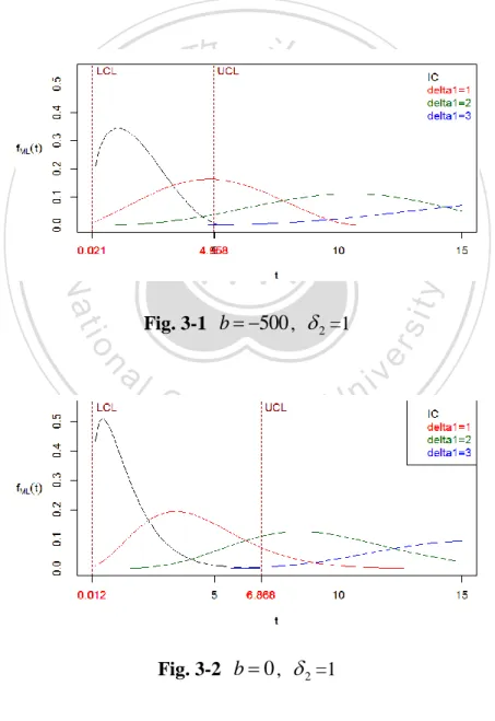
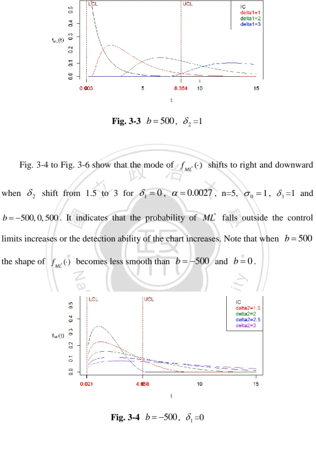
(30) Fig. 3-1 to Fig. 3-3 show the control limits of the ML chart and various pdfs of. ML* for 1 1, 2, 3 and 2 1 under 0.0027 , n=5, 0 1 , 3 =1 and b 500, 0, 500 respectively. The black curve is the in-control pdf of ML. Fig. 3-1 to. Fig. 3-3 show that the mode of f ML () shifts to right and downward when 1 goes *. from 1 to 3 under 2 1 , no matter what values of b . It indicates that the probability of ML* falls outside the control limits increases or the detection ability of the chart increases.. 立. 政 治 大. ‧. ‧ 國. 學. n. al. er. io. sit. y. Nat. Fig. 3-1 b 500 , 2 =1. Ch. engchi. i n U. Fig. 3-2 b 0 , 2 =1. 22. v.
(31) Fig. 3-3 b 500 , 2 =1. Fig. 3-4 to Fig. 3-6 show that the mode of f ML* () shifts to right and downward when 2. 政 治 大 shift from 1.5 立 to 3 for 0 , 0.0027 , n=5, 1. 0 1 , 3 =1 and. ‧ 國. 學. b 500, 0, 500 . It indicates that the probability of ML* falls outside the control. limits increases or the detection ability of the chart increases. Note that when b 500. ‧. the shape of f ML () becomes less smooth than b 500 and b 0 . *. n. er. io. sit. y. Nat. al. Ch. engchi. i n U. Fig. 3-4 b 500 , 1 =0. 23. v.
(32) Fig. 3-5 b 0 , 1 =0. 立. 政 治 大. ‧. ‧ 國. 學. Nat. n. sit er. io. al. y. Fig. 3-6 b 500 , 1 =0. i n U. v. Fig. 3-7 to Fig. 3-9 show that the mode of f ML () shifts rightward and. Ch. engchi. *. downward when 1 shifts from 1 to 3 for 2 3 , 0.0027 , n=5, 0 1 , 3 =1 and b 500, 0, 500 . It indicates that the probability of ML* fall outside the control limits increases, hence increases the detection ability.. 24.
(33) Fig. 3-7 b 500 , 2 3. 立. 政 治 大. ‧. ‧ 國. 學. Nat. n. sit er. io. al. y. Fig. 3-8 b 0 , 2 =3. Ch. engchi. i n U. Fig. 3-9 b 500 , 2 3. 25. v.
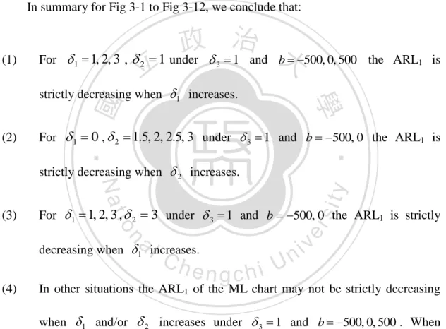
(34) Fig. 3-10 to Fig. 3-12 show that the mode of f ML () shifts leftward and *. downward when 2 shifts from 1.5 to 3 for 1 3 , 0.0027 , n 5 , 0 1 ,. 3 1 and b 500, 0, 500 . However, since the detection ability of the ML chart increases when the mode of f ML () goes rightward rather than leftward. It causes *. some ARL1 values not strictly decreasing while 2 increases. When either 1 or. 2 is large, the ARL1 values are all close to 1 and have no much difference. In summary for Fig 3-1 to Fig 3-12, we conclude that:. (1). For 1. 政 治 大 1, 2, 3 , 1 under 1 and b 500, 0, 500 立 2. 3. ‧ 國. (2). 學. strictly decreasing when 1 increases.. ‧. For 1 0 , 2 1.5, 2, 2.5, 3 under 3 1 and b 500, 0 the ARL1 is. sit. y. Nat. strictly decreasing when 2 increases.. n. al. er. For 1 1, 2, 3 , 2 3 under 3 1 and b 500, 0 the ARL1 is strictly. io. (3). decreasing when 1 increases. (4). the ARL1 is. Ch. engchi. i n U. v. In other situations the ARL1 of the ML chart may not be strictly decreasing when 1 and/or 2 increases under 3 1 and b 500, 0, 500 . When either 1 or 2 is large, the ARL1 values are all very close to 1.. 26.
(35) Fig. 3-10 b 500 , 1 =3. 立. 政 治 大. ‧. ‧ 國. 學. Nat. n. sit er. io. al. y. Fig. 3-11 b 0 , 1 =3. Ch. engchi. i n U. Fig. 3-12 b 500 , 1 =3. 27. v.
(36) To find how the ARL1 is influenced by 1 , 2 , 3 or b , the response table and diagram of average values of ARL1 ( ARL1 ) verses 1 , 2 , 3 or b are obtained in Table 3-3 and in Figure 3-13 based on the ARL1s for various combinations of 1 , 2 , 3 or b in Table 3-2. We found that, the ARL1 decreases when 1 or. 2 increases, and increases when b increases. The ARL1 is sensitive to the change of 1 and 2 , but is not sensitive to the change of 3 .. 政 治 大. Table 3-3 Response table for ARL1 of ML chart delta1. delta2. delta3. 1. 6.484. 4.278. 2.767. 1.460. 2. 3.747. 2.774. 2.803. 2.555. 3. 2.429. 2.282. 2.950. 4.493. 4. 1.759. 2.009. 2.913. -. 5. 1.397. -. 2.746. -. 1.198. -. -. n. al. Difference. C5.286 0.204 h e n 2.270 gchi U. y. sit. er. io 6. b. ‧. Nat. level. 學. ‧ 國. 立. vi n. 3.034. Fig. 3-13 Response diagram for ARL1 of ML chart 28.
(37) 3.1.2.2 Unbiased ARL Calculation for the Median Loss Chart. Pignatiello, et al. (1995) defined the concept of an ARL-unbiased control chart, as they state “the control chart is said to be ARL-unbiased if its ARL curve achieves its maximum when the process parameter is equal to its in-control value”. That is, the unbiased-ARL1 is always smaller than ARL0 even for asymmetric distributed monitoring statistics. However, the biased ARL1 do not have the reasonable property. Knoth and Morais (2013) proposed an ARL-unbiased S 2 chart and a EWMA- S 2 chart to monitor process dispersion, based on the concept of Pignatiello, et al. (1995).. 政 治 大. Pascual (2013) proposes combined individual and moving range charts based on. 立. ARL-unbiasedness for monitoring changes in either the Weibull scale or shape. ‧ 國. 學. parameter. So far using a single chart to joint monitor process mean and variance based on unbiased ARL has yet not been studied.. ‧ sit. y. Nat. Fig 3.14 shows the ARLs of the ML chart in (3-1). We can see that the ARL1s of. al. n. ARL1s are biased.. er. io. the ML chart are larger than ARL0 =370.4 for 2 1 2 and 2 1 . Hence the. Ch. engchi. 29. i n U. v.
(38) Fig. 3-14 Biased ARL of the ML chart. 政 治 大. ( 0.0027 , 0 0 , 0 1 , 3 0 and b 500 ). 立. ‧ 國. 學. To let the ML chart have reasonable ARL1 when 1 0 and/or 2 1 , we. ‧. need to adjust its control limits using the ARL-unbiased approach proposed by Sven. y. Nat. and Manuel (2013). Let ML and ML be the in-control mean and standard. n. al. UCL ML L2 ML. CLCLh L engchi ML. 1. ML. er. io. sit. deviation of ML, we redefine the control limits of the ML chart as. i n U. .. v. (3-5). The ML and ML in (3-5) can be calculated by letting. . . 0. 0. 2 ML t f ML (t | 0 , a0 , b , n, 3 )dt and ML (t ML ) 2 f ML (t | 0 , a0 , b , n, 3 )dt .. Consider the out-of-control process with 1 0 1 0 , 1 0 and 1 2 0 , 2 1 . Therefore the ARL-unbiased control limits coefficients L1 and L2 in (3-5). should satisfy the following three equations. 30.
(39) ARL0 1 ARL0 2. L1 , L2. 0,. (3-6). L1 , L2. 0,. (3-7). ARL0 L , L 1. 2. 1. . .. (3-8). The equation (3-8) ensures that the in-control ARL of the ARL-unbiased ML chart is 1 / , and the equations (3-6) and (3-7) are necessary conditions to let ARL0 is a local maximum.. 政 治 大. The Second Partial Derivative Test, for example see J. Stewart (2005), is applied. 立. to check whether the ( L1 , L2 ) values let ARL0 be a local maximum. Let D(0, 1) L , L 1 2. ‧ 國. 學. denotes the determinant of the Hessian matrix when critical point (1 , 2 ) (0, 1) , that. Nat 2. .. io. sit. 1. 2. (3-9). L1 , L2. er. D(0, 1) L , L. 2 2 2 ARL0 2 ARL0 ARL0 2 1 2 1 2 . y. ‧. is,. n. al. Ch. engchi. i n U. v. To check that the ARL0 is a local maximum, the Second Partial Derivative Test asserts 2 If D(0, 1) L , L 0 and 2 ARL0 1. 2. 1. 0.. (3-10). L1 , L2. We need to find the possible values of ( L1 , L2 ) satisfying (3-6), (3-7), (3-8) to let ARL0 be a local maximum. The computation procedures steps to find the final feasible values of ( L1 , L2 ) are described as below. 31.
(40) Step 1.. Since ARL0 . 1 1 is a function FML ( ML L1 ML ) 1 FML ( ML L2 ML ) . of ( L1 , L2 ) . From this equation one can obtain 1 FML ( ML L1 ML ) 1 ML FML. L2 . Step 2.. ML. .. (3-11). From (3-11) we can see that 0 FML ( ML L1 ML ) 1 1 . Then a nature domain of L1 is founded by 1 ML FML ( ) L1 ML . ML ML. 立. L2 .. ‧. ML. 學. 1 FML (1 ) ML. 1 For computation, we set ML FML ( ) L1 ML to find a large set of ML ML. er. io. sit. y. Nat. Step 4.. (3-12). Substitute (3-12) into (3-11) we obtain a nature domain of L2 given by. ‧ 國. Step 3.. 政 治 大. solutions of ( L1 , L2 ) such that ARL0 1 , and then screen out the . n. al. Ch. i e n gc hARL. solutions of ( L1 , L2 ) satisfying. 1. i n U . 0. . v. 2. ARL0 0 . A numerical. approach of these constraint is to satisfy ARL (1 e1 , 2 1) ARL (1 e1 , 2 1) ARL0 103 and 1 2e1. ARL (1 0, 2 1 e2 ) ARL (1 0, 2 1 e2 ) ARL0 103 . 2 2e2. The solutions of ( L1 , L2 ) were calculated by “nsga2” subroutine of R software. 32.
(41) From the values of ( L1 , L2 ) found in Step 4, we screen out the ( L1 , L2 ) values which can satisfy the following condition 2 ARL0 12. D(0, 1) L , L 0 and 1. 2. 0 L1 , L2. (the Second Partial Derivative Test represents that the ARL0 is a local maximum when 1 within 1 and 2 within 1 2 , 1 , 2 0 ). The D(0, 1) L , L is calculated by equation (3-9) with 1. 2. 政 治 大 ARL ( e e , 1) ARL ( e e , 立 2e. ARL ( 1 e3 e1 , 2 1) ARL ( 1 e3 e1 , 2 1) 2 ARL 0 2 2e1 1 1. 3. 1. 2. 1. 3. 1. 2. 1. 1) / 2 e3 , . 學. ‧ 國. ARL ( 1 0, 2 1 e4 e2 ) ARL ( 1 0, 2 1 e4 e2 ) 2 ARL0 2 2e1 2 ARL ( 1 0, 2 1 e4 e2 )) ARL ( 1 0, 2 1 e4 e2 ) / 2e4 , 2e1 . ‧. . io. sit. y. Nat. ARL ( 1 e1 , 2 1 e5 ) ARL ( 1 e1 , 2 1 e5 ) ARL0 1 2 2e1 2. . n. al. ARL ( 1 e1 , 2 1 e5 ) ARL ( 1 e1 , 2 1 e5 ) / 2e5 , 2e1 . er. Step 5.. Ch. engchi. i n U. v. where e1 e2 e3 e4 e5 104 .. Consider n 3 -51, 0 1 , 0.0027 , 3 0 , 1 and b 500 , 0, 500 respectively. The results are shown in Table 3-14. We found that the solutions of ( L1 , L2 ) can be obtained only when b 0 and 3 0 . However, in the cases with either b 500, 500 or 3 1 there is no solution.. 33.
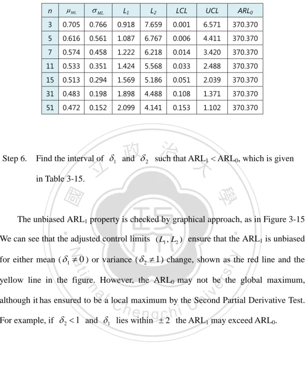
(42) Table 3-14 Control Limits of the Unbiased-ARL1 ML chart under b 0 and 3 0. Step 6.. n. ML. ML. L1. L2. LCL. UCL. ARL0. 3. 0.705. 0.766. 0.918. 7.659. 0.001. 6.571. 370.370. 5. 0.616. 0.561. 1.087. 6.767. 0.006. 4.411. 370.370. 7. 0.574. 0.458. 1.222. 6.218. 0.014. 3.420. 370.370. 11. 0.533. 0.351. 1.424. 5.568. 0.033. 2.488. 370.370. 15. 0.513. 0.294. 1.569. 5.186. 0.051. 2.039. 370.370. 31. 0.483. 0.198. 1.898. 4.488. 0.108. 1.371. 370.370. 51. 0.472. 0.152. 2.099. 4.141. 0.153. 1.102. 370.370. 政 治 大. Find the interval of 1 and 2 such that ARL1 < ARL0, which is given in Table 3-15.. 立. ‧ 國. 學 ‧. The unbiased ARL1 property is checked by graphical approach, as in Figure 3-15. We can see that the adjusted control limits ( L1 , L2 ) ensure that the ARL1 is unbiased. y. Nat. io. sit. for either mean ( 1 0 ) or variance ( 2 1 ) change, shown as the red line and the. n. al. er. yellow line in the figure. However, the ARL0 may not be the global maximum,. Ch. i n U. v. although it has ensured to be a local maximum by the Second Partial Derivative Test.. engchi. For example, if 2 1 and 1 lies within 2 the ARL1 may exceed ARL0.. 34.
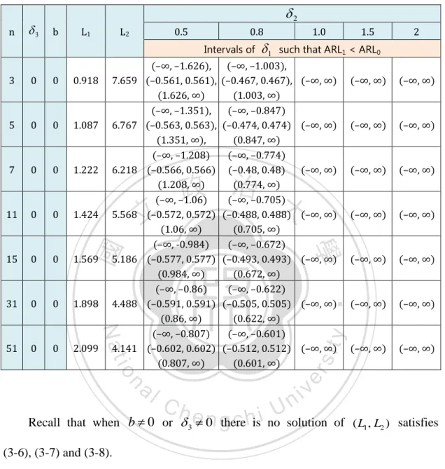
(43) (a) n 5. 立. 政 治 大(b). n 51. Fig. 3-15 The ARL of ARL1-unbiased ML chart. ‧ 國. 學. ( 0.0027 , 0 0 , 0 1 , 3 0 and b 0 ). ‧. y. Nat. Table 3-15 lists the ( L1 , L2 ) obtained in Table 3-14 and the corresponding. er. io. sit. interval of 1 such that ARL1 be unbiased under 0 0 , 0 1 , 3 0 , b 0 and. n. 2 0.5, 0.8, 1.0, 1.5, 2 respectively. We found the intervals a v of 1 in Table 3-15. i l C n h increases. becomes narrower when sample size engchi U. 35.
(44) Table 3-15 Values of ( L1 , L2 ) and the combination of 1 and 2 such that ARL1 < ARL0. L1. L2. 0.5. 0.8 Intervals of. 0.918. 5. 0. 0. 1.087. 7. 0. 0. 1.222. 11. 0. 0. 1.424. 15. 0. 0. 1.569. 31. 0. 0. 1.898. 51. 0. 0. 2.099. (–∞, –1.626), 7.659 (–0.561, 0.561), (1.626, ∞) (–∞, –1.351), 6.767 (–0.563, 0.563), (1.351, ∞), (–∞, –1.208) 6.218 (–0.566, 0.566) (1.208, ∞) (–∞, –1.06) 5.568 (–0.572, 0.572) (1.06, ∞) (–∞, -0.984) 5.186 (–0.577, 0.577) (0.984, ∞) (–∞, –0.86) 4.488 (–0.591, 0.591) (0.86, ∞) (–∞, –0.807) 4.141 (–0.602, 0.602) (0.807, ∞). 立. Nat. io. n. al. (–∞, –1.003), (–0.467, 0.467), (1.003, ∞) (–∞, –0.847) (–0.474, 0.474) (0.847, ∞) (–∞, –0.774) (–0.48, 0.48) (0.774, ∞) (–∞, –0.705) (–0.488, 0.488) (0.705, ∞) (–∞, –0.672) (–0.493, 0.493) (0.672, ∞) (–∞, –0.622) (–0.505, 0.505) (0.622, ∞) (–∞, –0.601) (–0.512, 0.512) (0.601, ∞). 政 治 大. ‧ 國. 0. Ch. engchi. 2. such that ARL1 < ARL0 (–∞, ∞). (–∞, ∞). (–∞, ∞). (–∞, ∞). (–∞, ∞). (–∞, ∞). (–∞, ∞). (–∞, ∞). (–∞, ∞). (–∞, ∞). (–∞, ∞). (–∞, ∞). (–∞, ∞). (–∞, ∞). (–∞, ∞). ‧. 0. 1.5. 學. 3. 1. 1.0. (–∞, ∞). (–∞, ∞). (–∞, ∞). (–∞, ∞). (–∞, ∞). y. b. (–∞, ∞). sit. 3. er. n. 2. i n U. v. Recall that when b 0 or 3 0 there is no solution of ( L1 , L2 ) satisfies (3-6), (3-7) and (3-8).. We may consider only the process mean change to preserve the unbiasedness of ARL1 of the ML chart, only (3-6) and (3-8) are applied. The new solutions of coefficients of control limits are called ( L1, L2 ) . The Second Derivative Test is applied to check ARL0 is a local maximum if only process mean change is considered.. 36.
(45) 2 The Second Derivative Test asserts that if 2 ARL0. 1. 0 , then ARL0 is a local L1 , L2. maximum when only mean change.. Table 3-16 lists the feasible values of ( L1, L2 ) by solving (3-6) and (3-8) and the corresponding intervals of 1 such that the ARL1 be unbiased for specified 2 under the combinations of n 3, 5, 7, 11, 15, 31, 51 , 0 0 , 0 1 , 0.0027 ,. 3 0, 0.5, 1 and b 500 , 0, 500 respectively. We found that the solutions of ( L1, L2 ) cannot be obtained when b 500 and. 政 治 大. n 51 , or when 3 0 and b 500 .. 立. ‧. ‧ 國. 學. n. er. io. sit. y. Nat. al. Ch. engchi. 37. i n U. v.
(46) Table 3-16 The Feasible Values of ( L1, L2 ) for Various Combinations of n, 1 , 2 ,. 3 and b such that ARL1 < ARL0. b. L 1’. L 2’. 0.5. 0.8 Intervals of. 0.920. 5.206. 5. 0. 0. 1.098. 4.889. 7. 0. 0. 1.253. 4.667. 11. 0. 0. 1.516. 4.371. 15. 0. 0. 1.740. 4.180. 31. 0. 0. 2.399. 3.793. 51. 0. 0. 2.926. 3.580. 3. 1. 0. 1.049. 5.732. 5. 1. 0. 1.231. 7. 1. 0. 1.374. (–∞, –1.228), (1.228, ∞) (–∞, –1.803), (1.803, ∞), (–∞, –1.005), (1.005, ∞) (–∞, –0.921) (0.921, ∞) (–∞, –0.876) (0.876, ∞) (–∞, –0.800) (0.800, ∞) (–∞, –0.765) (0.765, ∞) (–∞, –3.204), (–1.716, –0.284), (1.204, ∞) (–∞, –2.944), (–1.731, –0.269), (0.944, ∞), (–∞, –2.799) (–1.744, –0.256) (0.799, ∞) (–∞, –2.637) (–1.765, –0.235) (0.637, ∞) (–∞, –2.546) (–1.782, –0.218) (0.546, ∞) (–∞, –2.384) (–1.831, –0.169) (0.384, ∞) (–∞, –2.305) (–1.866, –0.134) (0.305, ∞). ‧ 國. 立. Nat. 5.286. io. 5.001. n. al. 11. 1. 0. 1.585. 4.648. 15. 1. 0. 1.733. 4.433. 31. 1. 0. 2.055. 4.018. 51. 1. 0. 2.243. 3.800. (–∞, –0.663), (0.663, ∞) (–∞, –0.627) (0.627, ∞) (–∞, –0.609) (0.609, ∞) (–∞, –0.591) (0.591, ∞) (–∞, –0.582) (0.582, ∞) (–∞, –0.568) (0.568, ∞) (–∞, –0.563) (0.563, ∞) (–∞, –2.633), (–1.843, –0.157), (0.633, ∞) (–∞, –2.489) (–1.870, –0.130) (0.489, ∞) (–∞, –2.411) (–1.866, –0.114) (0.411, ∞) (–∞, –2.325) (–1.906, –0.094) (0.325, ∞) (–∞, –2.277) (–1.919, –0.081) (0.277, ∞) (–∞, –2.196) (–1.946, –0.054) (0.196, ∞) (–∞, –2.157) (–1.962, –0.038) (0.157, ∞). 政 治 大. Ch. engchi U. 38. 2.0. (–∞, ∞). (–∞, ∞). (–∞, ∞). (–∞, ∞). (–∞, ∞). (–∞, ∞). (–∞, ∞). (–∞, ∞). (–∞, ∞). (–∞, ∞). (–∞, ∞). (–∞, ∞). (–∞, ∞). (–∞, ∞). (–∞, ∞). (–∞, ∞). (–∞, ∞). (–∞, ∞). (–∞, ∞). (–∞, ∞). (–∞, ∞). (–∞, ∞). (–∞, ∞). (–∞, ∞). (–∞, ∞). (–∞, ∞). (–∞, ∞). (–∞, ∞). (–∞, ∞). (–∞, ∞). (–∞, ∞). (–∞, ∞). (–∞, ∞). (–∞, ∞). (–∞, ∞). (–∞, ∞). (–∞, ∞). (–∞, ∞). (–∞, ∞). (–∞, ∞). (–∞, ∞). (–∞, ∞). er. 0. ‧. 0. 1.5. such that ARL1 < ARL0. 學. 3. 1. 1.0. y. 3. sit. n. 2. v ni.
(47) Table 3-16 (Continued). b. L 1’. L 2’. 0.5. 0.8 Intervals of. 5. 0.5 –500 1.467. 3.409. 7. 0.5 –500 1.592. 3.685. 11. 0.5 –500 1.777. 3.789. 15. 0.5 –500 1.906. 3.787. 31. 0.5 –500 2.189. 3.672. 51. 0.5 –500 2.353. 3.564. ‧ 國. 立. –500 1.429. 2.772. io. 1. Nat. 3. (–∞, –1.194), (–∞, –0.389), (–1.174, –0.449) (0.308, ∞) (0.698, ∞) (–∞, –1.466), (–∞, 0.118) (–1.218, 0.161) (0.344, ∞) (0.731, ∞) (–∞, –1.580), (–∞, 0.130) (–1.244, 0.171) (0.360, ∞) (0.726, ∞) (–∞, –1.650) (–∞, 0.123) (–1.282, 0.174) (0.591, ∞) (0.676, ∞) (–∞, –1.670), (–∞, 0.123) (–1.310, 0.181) (0.330, ∞) (0.637, ∞) (–∞, –1.670), (–∞, 0.130) (–1.371, 0.204) (0.292, ∞) (0.550, ∞) (–∞, –1.655), (–∞, 0.139) (–1.406, 0.223) (0.270, ∞) (0.502, ∞) (–∞, –2.191), (–∞, –0.013), (–1.713, –0.150) (0.303, ∞) (0.695, ∞) (–∞, –2.432), (–∞, –0.009), (–1.774, –0.143) (0.330, ∞) (0.698, ∞) (–∞, –2.525), (–∞, –0.015), (–1.826, –0.139) (0.326, ∞) (0.671, ∞) (–∞, –2.587), (–∞, –0.018), (–1.904, –0.123) (0.303, ∞) (0.613, ∞) (–∞, –2.600), (–∞, –2.328) (–1.959, –0.106) (–2.274, –0.015) (0.568, ∞) (0.282, ∞) (–∞, –2.585), (–∞, –2.427) (–2.076, –0.054) (–2.313, 0.002) (0.465, ∞) (0.232, ∞) (–∞, –2.558) (–∞, –2.452) (–2.143, –0.015) (–2.344, 0.016) (0.406, ∞) (0.203, ∞). n. al. 5. 1. –500 1.607. 3.175. 7. 1. –500 1.744. 3.339. 11. 1. –500 1.939. 3.445. 15. 1. –500 2.071. 3.464. 31. 1. –500 2.342. 3.420. 51. 1. –500 2.490. 3.362. 政 治 大. (–∞, ∞). (–∞, ∞). (–∞, ∞). (–∞, ∞). (–∞, ∞). (–∞, ∞). (–∞, ∞). (–∞, ∞). (–∞, ∞). (–∞, ∞). (–∞, ∞). (–∞, ∞). (–∞, ∞). (–∞, ∞). (–∞, ∞). (–∞, ∞). (–∞, ∞). (–∞, ∞). (–∞, ∞). (–∞, ∞). (–∞, ∞). (–∞, ∞). (–∞, ∞). (–∞, ∞). (–∞, ∞). (–∞, ∞). (–∞, ∞). (–∞, ∞). (–∞, ∞). (–∞, ∞). (–∞, ∞). (–∞, ∞). (–∞, ∞). (–∞, ∞). (–∞, ∞). (–∞, ∞). (–∞, ∞). (–∞, ∞). (–∞, ∞). (–∞, ∞). (–∞, ∞). (–∞, ∞). er. 2.781. Ch. engchi. 39. 2.0. such that ARL1 < ARL0. ‧. 0.5 –500 1.297. 1.5. 學. 3. 1. 1.0. y. 3. sit. n. 2. i n U. v.
(48) Fig. 3-16 (a) shows the ARL of the biased-ARL1 ML chart and the unbiased-ARL1 ML chart with adjusted ( L1, L2 ) for 2 1 2 , 2 1 , n 5 ,. 0 0 , 0 1 , 0.0027 , 3 0.5 and b 500 . The solid red line represents the unbiased ARL1, and the dark-blue dashed line represents the biased ARL. We found that the unbiased ARL1 is smaller than ARL0=370.4 but biased ARL1 does not when only process mean change.. Figure 3-16 (b) shows the ARL1s of the ML chart with coefficients of the control limits ( L1, L2 ) under 3 1 3 and 0.1 2 3 , n 5 , 0 0 , 0 1 ,. 0.0027 , 3. 政 治 大 0.5 and 立b 500 . We can see that when . 1. 0 and 2 0.5. ‧. ‧ 國. satisfy (3-7).. 學. the ARL1 may be biased. Since the coefficients ( L1, L2 ) of the control limits do not. n. er. io. sit. y. Nat. al. Ch. engchi. (a) ARL1 when 2 1 2 , 2 1. i n U. v. (b) ARL1 when 3 1 3 , 0.1 2 3. Fig. 3-16 The ARL of the adjusted ML chart parameters ( L1, L2 ) under , n 5 ,. 0 0 , 0 1 , 0.0027 , 3 0.5 and b 500. 40.
(49) 3.1.2.3 ARL1 Comparison between the Biased ARL and Unbiased ARL of the Median Loss Charts. The ARL values comparing among these three methods are given in Table 3-17, the three methods are (1) The ARL1-unbiased method with partial derivative of 1 and 2 (2) The ARL1-unbiased method with only partial derivative of 1 and fixed. 2 1 (3) The ARL1-biased ML chart. From Table 3-17 we can see that, “method 1” ensures that ARL1 smaller than ARL0 for either mean or variance change; “method 2” ensures that unbiased-ARL1. 治 政 smaller than ARL if we consider only process mean大 change; “method 3” leads the 立 biased-ARL to be larger than ARL if either mean and/or variance changes. On the 0. 1. 0. ‧ 國. 學. other hand, if 1 1 and 2 1.5 , the detection ability or ARL1 of these three. ‧. methods have no much difference. A more detailed discussion of comparing these three methods is listed in Table 3-18.. n. er. io. sit. y. Nat. al. Ch. engchi. 41. i n U. v.
(50) Table 3-17 The ARL1 comparison between ARL1-biased and unbiased ML charts ( n 5 , 0 0 , 0 1 , 0.0027 ) b 0, 3 1. 0. 1. 370.37. 370.37. 370.37. 370.37. 370.37. 370.37. 370.37. 370.37. 370.37. 0.2. 1. 367.930. 295.189. 332.322. 265.741. 204.742. 67.558. 43.311. 68.922. 39.014. 1. 1. 47.457. 16.196. 24.152. 10.279. 8.146. 2.365. 2.182. 2.276. 2.059. 0. 0.2. 5.787. -. 8.836. -. 1.50e+15. -. 2252.547. -. 2.63e+08. 0. 0.5. 61.494. -. 101.295. -. 7435.591. -. 293.793. -. 1884.877. 0. 0.8. 231.401. -. 382.283. -. 806.521. -. 491.949. -. 735.808. 0. 1.5. 30.070. -. 17.962. -. 37.716. -. 5.600. -. 7.494. 1. 1.5. 9.529. 5.290. 6.591. 5.137. 4.528. 1.805. 1.727. 1.885. 1.781. 2. 1.5. 2.193. 1.687. 1.854. 政 治 大 1.540. 1.465. 1.149. 1.135. 1.152. 1.135. 3. 1.5. 1.150. 1.078. 1.101. 1.055. 1.045. 1.022. 1.019. 1.021. 1.018. 1. 2. 4.202. 2.880. 3.317. 3.656. 3.355. 1.510. 1.467. 1.639. 1.576. 2. 2. 1.998. 1.630. 1.757. 1.621. 1.554. 1.161. 1.148. 1.185. 1.168. 3. 2. 1.238. 1.147. 1.178. 1.124. 1.109. 1.043. 1.039. 1.047. 1.042. 1. 3. 1.944. 1.620. 1.734. 2.277. 2.163. 1.237. 1.220. 1.342. 1.313. 2. 3. 1.577. 1.386. 1.454. 1.590. 1.541. 1.122. 1.113. y. 1.166. 1.153. 3. 3. 1.276. 1.186. 1.218. 1.233. 1.213. 1.057. 1.053. 1.075. 1.069. 2. 0.5. 2.829. 1.361. 1.144. 1.085. 1.01. sit. b 500, 3 1. ‧ 國. b 500, 3 0.5. 2. ‧. b 0, 3 0. 1. 1.007. 1.008. 1.005. 2. 1. 2.35. 1.604. 1.395. 1.313. 1.077. 1.081. 1.067. 3. 0.5. 1.000. 1.000. 1.000. 1.000. 1.000. 3. 1. 1.049. 1.015. C h1.000 1.000 1.000 engchi 1.024 1.008 1.005. i n U1.000 1.003. 1.003. 1.003. 1.002. -3. 0.5. 1.000. 1.000. 1.000. 1.008. 95.804. 1.000. 1.000. 9.539. 7.008. -3. 1. 1.049. 1.015. 1.024. 1.306. 8.146. 1.202. 1.164. 4.853. 4.251. -2. 1. 2.350. 1.604. 1.829. 5.454. 370.370. 5.219. 4.716. 19.420. 27.231. -1. 1. 47.457. 16.196. 24.152. 130.092. 175.217. 47.213. 53.277. 57.786. 106.498. -0.2. 1. 367.930. 295.189. 332.322. 300.810. 374.662. 246.226. 390.035. 241.236. 461.946. Method 1 Method 2 Method 3 Method 2 Method 3 Method 2 Method 3 Method 2 Method 3. io. n. al. 1.829. 42. 學. Nat. 1.687. er. 立. 1.088. v.
數據
+7
相關文件
The closing inventory value calculated under the Absorption Costing method is higher than Marginal Costing, as fixed production costs are treated as product and costs will be carried
• When a system undergoes any chemical or physical change, the accompanying change in internal energy, ΔE, is the sum of the heat added to or liberated from the system, q, and the
Students are expected to explain the effects of change in demand and/or change in supply on equilibrium price and quantity, with the aid of diagram(s). Consumer and producer
Reading Task 6: Genre Structure and Language Features. • Now let’s look at how language features (e.g. sentence patterns) are connected to the structure
Promote project learning, mathematical modeling, and problem-based learning to strengthen the ability to integrate and apply knowledge and skills, and make. calculated
2.8 The principles for short-term change are building on the strengths of teachers and schools to develop incremental change, and enhancing interactive collaboration to
Wang, Solving pseudomonotone variational inequalities and pseudocon- vex optimization problems using the projection neural network, IEEE Transactions on Neural Networks 17
Define instead the imaginary.. potential, magnetic field, lattice…) Dirac-BdG Hamiltonian:. with small, and matrix
