內生查獲機率及內生Cartel形成下之Cartel價格動態

(1)

行政院國家科學委員會專題研究計畫成果報告

內生查獲機率及內生 Cartel 形成下之 Cartel 價格動態

研究成果報告(精簡版)

計畫類別：個別型

計畫編號： NSC 99-2410-H-004-053-

執行期間： 99 年 08 月 01 日至 100 年 07 月 31 日

執行單位：國立政治大學財政系

計畫主持人：陳國樑

計畫參與人員：碩士班研究生-兼任助理人員：李政翰

碩士班研究生-兼任助理人員：鄭岳旻

博士班研究生-兼任助理人員：黃勢璋

博士班研究生-兼任助理人員：王慧華

博士班研究生-兼任助理人員：陳揚仁

博士班研究生-兼任助理人員：陳韻旻

公開資訊：本計畫涉及專利或其他智慧財產權，2 年後可公開查詢

中華民國 100 年 10 月 31 日

(2)

中文摘要：本篇研究提出了一個 cartel 價格動態的模型。模擬 cartel 的價格

路徑顯示， cartel 的價格攀升可分成兩個階段。首先，在過渡

性階段，無視於成本之變化，價格持續上升。其次，經過若干

過渡期後，價格進入安定性階段，且隨成本之變動而調整。此

點結論與 Harrington and Chen (2006) 大致相同。價格變動相較

於成本變動之迴歸結果顯示，cartel 對成本上升之反應大過其對

成本下降之反應。此一情形在過渡性階段尤其明顯，面對成本

上升時，cartel 的價格向上調整的幅度遠大於成本下降時其價格

向下調整的幅度。在安定性階段，cartel 對於成本上升或下降的

價格反應大致相同。

英文摘要： This study has a model that generates a richer set of predictions

about cartel pricing dynamics. In line with Harrington and Chen

(2006), the simulated price paths suggest that the up-rising of the

cartel price is comprised of two phases. Starting from a transitional

phase, the price is generally rising and relatively unresponsive to

cost shocks. Then the price moves to a stationary phase where price

responds to cost. The price change vs. cost change regressions

suggest that a cartel is more responsive to cost increases than to cost

decreases. In the transitional phase, the cartel raises price more than

predicted when cost shocks are positive and lower price less than

predicted when cost shocks are negative. As to the stationary phase,

the cartel responds to positive and negative cost shocks equally.

(3)

NSC Research Project (99-2410-H-004-053-) Summary

Report: Cartel Pricing Dynamics with Endogenous

Probability of Detection

Joe Chen

October 31, 2011

Abstract

This study has a model that generates a richer set of predictions about cartel pricing dynamics. In line with Harrington and Chen (2006), the simulated price paths suggest that the up-rising of the cartel price is comprised of two phases. Starting from a transitional phase, the price is generally rising and relatively unresponsive to cost shocks. Then the price moves to a stationary phase where price responds to cost. The price change vs. cost change regressions suggest that a cartel is more responsive to cost increases than to cost decreases. In the transitional phase, the cartel raises price more than predicted when cost shocks are positive and lower price less than predicted when cost shocks are negative. As to the stationary phase, the cartel responds to positive and negative cost shocks equally. [Keywords: Cartel Pricing Dynamics, Endogenous Probability of Detection]

(4)

1 Aim of Research

The major challenge to stopping cartels is that they are shrouded in secrecy. From an an-titrust perspective, the essential tasks for a theory of price-fixing are identifying conditions that facilitate collusion, characterizing the properties of collusive pricing, and towards dis-cerning the presence of a cartel. Although there is a large theoretical literature addressing these issues, work has generally failed to take account of an important dimension to this problem. Due to the illegality of collusion, firms not only want to achieve internally stable prices to raise profit but also want to avoid creating suspicions that a cartel is in action. Given that such suspicions can initiate investigation from the antitrust authority that can ultimately lead to the collapse of the cartel and levying of substantial financial penalties, avoiding detection is as crucial as deterring deviations by cartel members.

Arguably, modern theory of collusive pricing originates from models of tacit (implicit) collusion with the idea of deterring deviations among rival firms in an oligopolistic setting (Porter, 1993; Green and Porter, 1984; Rotemberg and Saloner, 1986). Feuerstein (2005) surveys a rich collection of articles in this literature; Athey et al. (2004) have a brief intro-duction to the development of this literature with a particular interest in the information structure. Nonetheless, in terms of antitrust pursuit of hardcore cartels, the contribution of the tacit collusion literature is limited in that, first, works generally do not explain how does a hardcore cartel actually function under the constraint of possible detection; second, tacit collusion is not illegal, at least in the U.S. and European Union.1 Martin

(2006) expresses this concern stating that: “there is a fundamental disconnect between treating collusion as the outcome of a noncooperative game and the antitrust concept of

1_{Implicitly, the Horizontal Merger Guidelines (Section 2.1) of the Department of Justice Federal Trade}

Commission gives authority to assess if a merger increases the possibility of coordinated interaction which includes both tacit and express collusion. For more discussions on the legal status of tacit collusion see Martin (2006) and Harrington (2005b).

(5)

collusion,” and “models of tacit collusion are fundamentally unsuited for the analysis of collusion.” In light of these critics, this research proposal suggests a computational model of hardcore cartel behavior in the presence of antitrust authority.

A recent strand of the collusive pricing literature explores the impact of antitrust enforcement on collusive pricing by modifying the classical repeated-game setting so as to allow the detection of a cartel to be sensitive to the price path (endogenous detection). This changes the traditional framework of antitrust analyses where penalty and probability of detection are exogenous to cartel behavior (for the origin of this new strand of literature see Harrington, 2004 & 2005a). In particular, Harrington and Chen (2006) characterize collusive pricing patterns when buyers may detect presence of a cartel. Buyers are modeled to become suspicious when observed prices are anomalous.2 _{The model is successful in}

that it generates cartel price paths that look more like actual cartel price paths than any previous work in the theoretical literature on collusive pricing.

This study picks up this latest strand to develop a better theory of cartel pricing. A key in Harrington and Chen’s work is the buyers’ beliefs in whether the price changes are “regular”. However, due to computational constraints, they assume the variance of buyers’ beliefs over price changes to be fixed at the variance of price changes for the non-collusive environment. This rules out the realistic scenario that the variance of price changes may adjust to firms’ prices, and the sensitivity of the likelihood of price changes would evolve over time. In other words, despite a rather general dynamic framework, buyers’ beliefs over price changes are “static” in the sense that the second moment of likelihood is fixed.

2_{As Harrington and Chen (2006) point out, as a matter of practice, the antitrust authorities, given}

the constraint in resources, do not actively engage in detection. But instead, it is often the buyers– industrial buyers in particular–who are on the first line of detection in many cartel cases. For example, see Levenstein and Suslow (2001) for the case of the graphite electrode cartel, Levenstein, Suslow, and Oswald (2004) for the case the stainless steel cartel, and Ashenfelter and Graddy (2004) for some discussions on the Sotheby’s/Christie’s price-fixing scandal.

(6)

This concern casts a doubt on how does a more general and realistic setup changes the results, and whether will there be new aspects come out of a fully-fledged dynamic setting? This study designs to tackle this problem by modeling the buyer belief formation process explicitly. The idea is to allow buyers’ beliefs over price changes to depend on noisy cost signals. In many markets, buyers receive noisy signals of the underlying cost shocks. For example, consider the vitamins cartel. As vitamins are manufactured in Europe and sold in the U.S., exchange rate fluctuations are publicly observable cost shocks. One can then imagine buyers assessing whether the price change is “reasonable” in light of the information received about the change in costs. The innovative element of this approach is that it modifies the standard (repeated game) model of collusion to allow a cartel to actively avoid detection by choosing its prices optimally in an environment with cost variability and endogenous buyer belief formation.

2 Model Setup

2.1 Cartel Pricing Dynamics with Endogenous Probability of

De-tection

The main modeling challenge, as alluded above, is to formulate the buyers’ belief formation process. I propose to allow buyers’ beliefs over price changes to depend on noisy cost signals. In particular, one can assume a recursive identification algorithm (Ljung and Söderström, 1983) so that there is an equation of motion on buyer’s “model” of price changes which depends on the previous period’s model of price changes and the current period’s price change and cost shock signal. Once specifying a distribution on those prediction errors, we can then define the relative likelihood of a series of prediction errors to characterize anomalous price changes.

(7)

2.2 Buyers’ Side

Consider a time series of “data”, comprised of price changes 4_{and noisy signals }_{, and}

buyers would like to make judgement on whether firms behave competitively. Not actively engaging in collusion detection, buyers do not know how a cartel prices. Nonetheless, they do have a model of competitive (non-collusive) pricing that specifies period  price change 4_{as a linear function of the corresponding period  cost change 4}_.

However, in each period, instead of observing 4_{directly, buyers receive a noisy signal}

_{of 4}_{. Based on their model of competitive pricing and the signal, buyers calculate the}

predicted price change. When the competitive pricing model cannot explain the actual price change well (e.g., the signal is rather noisy or a cartel is in action to raise the price significantly, or both), an active cartel is more likely to be exposed. Hence, the detection of the cartel is more likely to occur when there is a “large” prediction error. Each period, the actual price change 4 _{and the received signal } _{are new data used by buyers to}

update parameters of the competitive pricing model. This updating is performed by a recursive algorithm in an on-line fashion.

For what stated above, let buyers believe the competitive price changes follow this process:3

4=  + 4+ 

3_{When  6= 0, there is a trend in buyers’ model of competitive pricing. It is quite reasonable for buyers}

to believe there is a trend in price. In some industries (such as computers and electronic products), the real price falls–perhaps due to innovation or the learning curves. In other industries, the real price rises. Even if the average price change in the economy is zero, there is dispersion in price trends among industries which means some must have the real price rising and some have it falling. In the context of the setting here, there is no reason for buyers to expect price to remain constant in light of a changing environment; they do not know that the average cost shock is zero for all they get to observe are noisy cost signals and the price change.

(8)

where 4_{∼ (0 }2

) and ∼ (0 2) and is i.i.d.4 Buyers receive a noisy signal of the

cost shock:

_{= 4}+ 

where  _{∼ (0 }2_) and is i.i.d. Buyers’ model for period  price change can then be written as:

d

4=_b+ b

where _b _{and b}_ _{are buyers period  estimation of the true parameters,  and , of the}

competitive pricing process.

2.3 The Cartel’s Problem

At the beginning of period , the state variables are ³−1_{ }−1__b_{ b}_´_{. After seeing}

period  cost shock, 4_{, the cartel chooses price change, 4}_{. The cartel’s value function}

 (·) is defined recursively by: ³_4; −1 −1_b b´ ≡ max 4 ¡ −1_{+ 4} ¡−1_{+ 4}¢¢ + ZZ n ³_4_{ 4}+ _b b´ £¡¡−1_{+ 4}¢¢_{− }¤+h_{1 − }³_4_{ 4}+ _b bí × µ ; −1_{+ 4} ¡−1_{+ 4}¢_b+ 1  h 4−³b_{+ b}_¡ 4+ ¢í b₊ 4+  ³2 + 2 ´h4−³b_{+ b}_¡ 4+ ¢í ⎞ ⎠ ⎫ ⎬ ⎭ ¡ ; 0 2_¢¡; 0 2_¢ = max 4 ¡ −1_{+ 4} ¡−1_{+ 4}¢¢ + Z ³_4_{ 4}+ _b b´¡; 0 2_¢_{ ·}£¡¡−1_{+ 4}¢¢_{− }¤ + ZZ nh 1 − ³4 4+ _b bí¡; −1_{+ 4} ¡−1_{+ 4}¢ b₊1  h 4−³b_{+ b}_¡ 4+ ¢í b+ 4 _{+ } ³2 + 2 ´h4−³b_{+ b}_¡ 4+ ¢í ⎞ ⎠ ⎫ ⎬ ⎭ ×¡; 0 2_¢¡; 0 2_¢

(9)

where (·) is the current period industry profit function,  (·) is the probability of detec-tion,  (·) is the non-collusive profit stream, and (·;  2_{) is the normal density function.}

The specifications of (·), (·),  (·), and  (·) are:  () ≡ max { min { }} ;  ( ) ≡ ( − ) ( −  ) ; ³_4_{ 4}+ _b b´_≡ ⎧ ⎪ ⎪ ⎪ ⎨ ⎪ ⎪ ⎪ ⎩ 0+ 1 ∙  (0;02)−(4−−(4+);02)  (0;02) ¸ 2 if 4_{− b}_{− b}_(4_{+ ) ≥ 0} 0+ 1 ∙  (0;02)−(4−−(4+);02)  (0;02) ¸ 2 if 4_{− b}_{− b}_(4_{+ )  0} ;  () ≡³ () − b ´ ³ −  b ()´+ Z  ((+))¡; 0 2_¢ with competitive price b () = 0+ 1.

The parameters in the definition include³     0 1 2 1 2 0 1   2 2 2

´ .   0 is the penalty when detected (and convicted);   0 is the number of periods in

buyers’ memory, ,   0 are demand parameters;  ∈ (0 1) is the discount factor; (0 1 2 1 2) are detection function parameters; (0 1) ∈ [0  (2)) × (12 1]

characterizes the competitive price;  and  are bounds on the unit cost of production; 2

 is the variance of cost shocks; 2 characterizes the degree of noisiness in the buyer’s

signal; 2 is the second moment of prediction errors.

The main objective of this exercise is to explore the relationship between cost changes, 4, and cartel’s price changes, 4 . The setup of the sequence of events is one such that the cartel gets to see the cost shock 4before choosing price 4but does not get to see the noisy signal, , that the buyers observe. In other words, cartel chooses price change

(10)

3 Numerical Implementation

The existence of symmetric subgame perfect equilibrium can be established along the same line of reasoning as given in Harrington (2004). Nonetheless, given the complexity of the models and the lack of analytical solutions in many dynamic programming problems, the cartel’s problem is solved numerically through the collocation method (Judd, 1998; Miranda and Fackler, 2002) which replaces the diﬃcult infinite-dimensional functional equation with a simpler finite-dimensional problem. The essence of this algorithm is, conceptually, a straightforward application of the value function iteration method. Just as examples of how the collocation method works in these types of models, please refer to Chen and Harrington (2007), and the appendix sections in Harrington (2004) and Harrington and Chen (2006).

3.1 Benchmark Parameters

• Demand function:  −  . Set ( ) = (100 1) • Cost parameters; ( ) = (20 40)

(11)

approxi-mated by a 5-point Gaussian quadrature with (_ 2

) = (0 2):5

quadrature nodes quadrature weights

-4.0404 .0113

-1.9171 .2221

0 .5333

1.9171 .2221

4.0404 .0113

• The non-collusive payoﬀ function  () is solved numerically by the functional iter-ation method. The discretized cost space for  () is 51 evenly distributed points from the interval [ ]. The result suggests  (·) is a monotonic decreasing function. • Discount factor:  = 75.

• Non-collusive price parameters: (0 1) = (25 75)

• Damages:  = 490. Denote the average cost as e ≡ ( + )2. Let (_{e) be the} monopoly price at average cost: ₍

e) = ( + e)2. The fixed fine  is set according to:  = 1 10· (₍_e)) 1 −  = 1 10·

(₍_{e) − e)( − }₍_e))

1 −  

• Probability of detection parameters: (0 11 2 2) = (05 45 2 2 2).

• Buyers’ parameters: the number of periods in buyers’ memory  = 10; the variance of the noise in the signal 2_ = 1.

• The distribution of buyers’ prediction error is (0; 0 2). Set 2= 3.6

5_{The number of the quadrature nodes is the same as the number of nodes of 4 in the value function}

 (·). This means that the choice of a large number of quadrature nodes would cause a burden in solving the value function–the so-called curse-of-dimensionality problem.

6_{Originally, the model is set up in a way that }

2is endogenous, and 2 is defined by:

2= −1   =− ()2=  1   _−1  =−  4−_{+ }__2_,

(12)

• Noise distribution: (;  2). This distribution is also approximated by a 5-point

Gaussian quadrature with (_ 2

) = (0 1):7

quadrature nodes quadrature weights

-2.8570 .0113

-1.3556 .2221

0 .5333

1.3556 .2221

2.8570 .0113

• The value function  (·) is a function of 4_{, }−1_{, }−1_,_b_{, and b}__{. The space of the}

value function is assigned in the first row of the following table. Given the assigned ranges, the 5 × 5 Chebychev nodes are:

4_{∈ [−7 7]} _−1_{∈ [20 80]} _−1_{∈ [20 40]} _b_{∈ [−5 5]} b_{∈ [0 2]} −66574 21468 20489 _−4755 00489 −41145 32366 24122 _−2939 04122 0000 50 30 0000 1 41145 67634 35878 2939 15878 66574 78532 39511 4755 19511

To get a more concentrated range −1_{, the price nodes are changed to {30 40 50 60 70}.}

• The choice set is a 39-point discretized space of price changes, 4 , from −3 to 3.

and _{is an estimate of }_{≡ }_{− }

∼ 0 2 + 22



. Since _{∈ [ ], the appropriate range for the}

state variable  2 is: 2∈ [2+ 22 2+  2 2] When (  2  2) = (0 2 1 1), 2∈ [1 5].

7_{Note that unlike the choice of quadrature nodes of the cost shocks, one may increase the nodes of}

 (;  2)to a 10-point (or higher) Gaussian quadrature without causing the cure-of-dimensionality

(13)

• The variables in value function  (·) move according to: 4 ←  −1 _{← }−1_{+ 4}_{≡ } −1 _{← (}−1_{+ 4}_{) ≡ } b ← b+1  h 4−³b_{+ b}_¡ 4+ ¢´i_{≡ b}+1 b ← b+ 4 _{+ } ³2 + 2 ´h4−³b_{+ b}_¡ 4+ ¢´i_{≡ b}+1

To ensure that the numerical algorithm converges, one needs to make sure that the new variables remain in the specified state space. There is no need to worry about  (possible future cost shocks) and (4_{+ ) because the nodes of  are inside}

the range specified by the the nodes of 4_{, and because (·) ∈ [ ] by definition.}

One can also ensure that −1 _{+ 4} _{remains in the specified range as long as}

  −1 _{  and 4}is small. Nonetheless, there are no guarantees that _b+1 and b+1 _{will remain in the respective specified ranges. There are a few things one}

can do, such as choosing a larger value for , or considering a smaller range of price change 4 , but the problem remains. In order to get a converge result, the updating rules of_{b and b are changed to:}

b ← b+1= max{−5 min{b+1  h 4−³b_{+ b}_¡ 4+ ¢´i_{ 5}}} b ← b+1= max{0 min{b+ 4 _{+ } ³2 + 2 ´h4−³b_{+ b}_¡ 4+ ¢´i_{ 2}}}

The concern is on how restrictive that these new updating rules of_{b and b are.}8

8_{It seems diﬃcult to get a complete picture of this issue. There are 5}5_{= 3 125}_{states, and for each}

possible cost shock (), there are five possible signal noises (). Since the choice space (price change) is a 39-point discretized interval of [−3 3], +1_{and }_+1_{are both matrices with dimension 3 125 × 25 × 39.}

For our purpose, we simply take the value function computed from the benchmark parameter specification to price simulations. Later, we can then draw the paths of and  to see how they evolve, and the roles played by the max and min operators in the updating rule.

(14)

3.2 Price Path Simulation

After solving the cartel’s maximization numerically, simulating cartel behavior is straight-forward. Let the choice set be the 121-point discretized interval [−3 3]. Set the initial values of the state variables to: (0 0_b1 b1) = (475 30 0 1), where 0 = 0+ 10,

the non-collusive price at 0_{= ( + )2. The choices of initial values of }0__b1_{, and b}_1_are

based on the assumption that at period zero, consumers have no reason to believe that the cartel is active. In each period , the timing of events in the price path simulation is as follows:

• A random cost shock 4 _{is draw from the distribution  (; 0 }2 );

• The cartel maximizes discounted expected profit choosing 4from the choice set, conditional on 4 and state variables −1 −1_b, and b. The expectation is taken with respect to the probability of been detected, (·), future cost shock, , and the noise in the consumer’s signal, ;

• A signal noise is drawn from the distribution  (; 0 2 );

• Given 4_{, 4}_{, and }

, we then update the state variables to (_{ }__b+1_{ b}_+1₎

based on the equations of motion of these variables and move on to the next period.

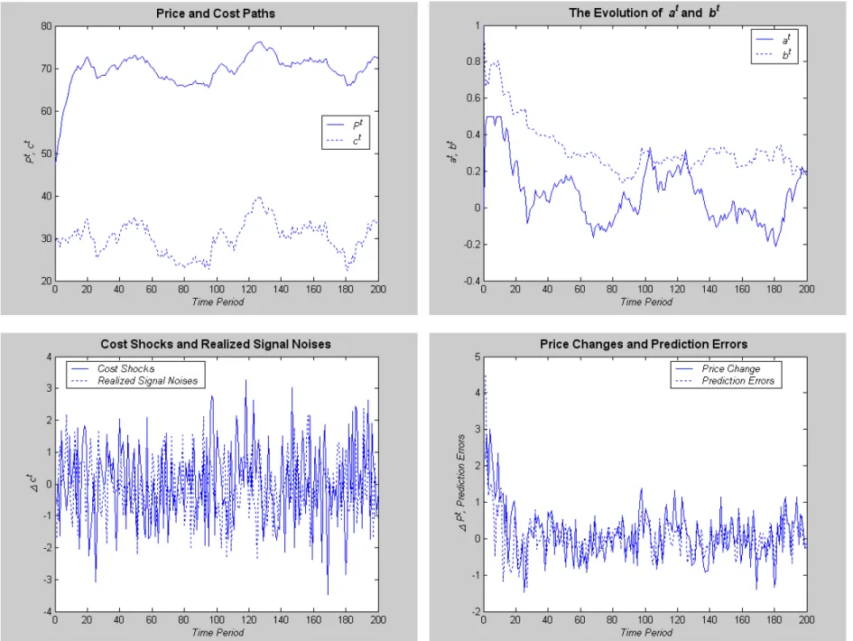
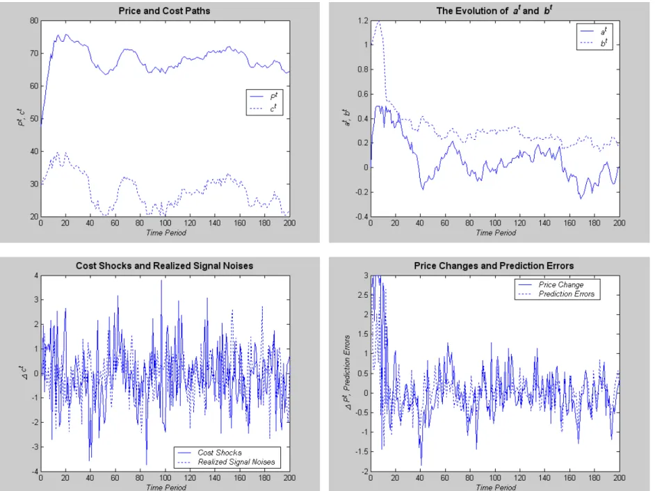
The number of periods is set to 200; Figure 1 presents three–Runs I—III–price path simulation results. For the result of each price simulation, the top-left figure presents the price path  _{and the cost path }_{, the top-right figure shows the evolutions of} _b

and b_{, the bottom-left figure shows the cost shocks 4}_{, and the realized signal noises}

_{, and the bottom-right figure presents the price change 4} _{and the prediction errors}

4₋h_b_{+ b}__(4_{+ }

)i.

The simulated price paths suggest that the up-rising of the cartel price is comprised of two phases. Beginning with a transitional phase, the price is generally rising and

(15)

relatively unresponsive to cost shocks. Then the price moves to a stationary phase where price responds to cost. In a richer dynamic environment, this result is in line with that in Harrington and Chen (2006).

4 Discussion

Notice first that if the price evolves according to non-collusive pricing rule, = 0+1,

this implies 4 = 14, and based on the benchmark parameters, ( ) = (0 75).

If the price is set to the single period monopoly level, it implies 4 = (12)4, and ( ) = (0 5). If firms practice constant markup pricing,  = , this implies 4 = 4, and  = 0 and   1. In perfect competition,  = , this implies 4 = 4, and ( ) = (0 1).

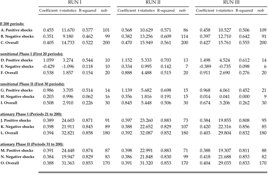
Given the simulated price paths, we regress the current price change on the change in cost based on the following equation:

4_{= 4}_{+ }_

where _{is a white noise. Furthermore, regressions are also done distinguishing between}

positive and negative cost shocks. In addition, we also do the regressions using “data” from the transitional periods only–one set uses the first 20 periods, and the other set uses the first 30 periods. Finally, we also conduct stationary phase regressions–the first set uses data from period 21 to period 200, and the other the other uses data from period 31 to period 200. All these results are presented in Table 1.

With data from all 200 periods, the estimated coeﬃcients of cost shocks are .41, .47, and .43, respectively for Runs I, II, and III. It is interesting to note that these values are close to .5, the single period monopoly . If we distinguish positive or negative cost shocks, the estimated coeﬃcients of cost shocks are .46, .57, and .46, for positive cost shocks, and .35, .38, and .40 for negative cost shocks. All the estimates are significant.

(16)

With data from the first 20 periods, the estimated coeﬃcients of cost shocks are .54, .89, and .91, respectively for runs I, II, and III. If we distinguish positive or negative cost shocks, the estimated coeﬃcients of cost shocks are 1.06, 1.15, and 1.50, for positive cost shocks, and -.43, .33, and -0.39 for negative cost shocks. All the estimates of the negative cost shock regressions are insignificant.

With data from the first 30 periods, the estimated coeﬃcients of cost shocks are .51, .85, and .67, respectively for runs I, II, and III. If we distinguish positive or negative cost shocks, the estimated coeﬃcients of cost shocks are .99, 1.14, and .97, for positive cost shocks, and .21, .36, and .01 for negative cost shocks. Again, all the estimates of the negative cost shock regressions are insignificant.

Based on these results, this study has a model that generates a richer set of predictions about cartel pricing dynamics. It is clear from the regressions that the cartel is more responsive to cost increases than to cost decreases. In particular, in the transitional phase, the regressions all have coeﬃcient estimates around 1 when the cost shocks are positive, while at the same time negative cost shocks cannot explain the price changes at all. Comparing the transitional phase regression results with those of the stationary phase, it is apparent that in the transitional phase, the cartel raises price more than predicted when cost shocks are positive and lower price less than predicted when cost shocks are negative. This allows the cartel to raise price during the transitional phase. As to the stationary phase, the cartel responds to positive and negative cost shocks equally; the above asymmetry does not exist.

In summary, the results of this project contribute to the literature of industrial orga-nization in characterizing the properties of collusive pricing and in identifying conditions that facilitate collusion. They fill in the hole in the current literature of collusive pricing which ignores the important incentive of cartel members price to avoid detection. Using the price simulation results, one can identify important traits in discerning the presence of

(17)

a cartel, accessing the eﬀectiveness of antitrust practice, and developing screening mech-anism for the existence of a cartel.

References

[1] Ashenfelter, Orley and Kathryn Graddy, 2005, Anatomy of the Rise and Fall of a Price-Fixing Conspiracy: Auctions at Sotheby’s and Christie’s, Journal of Competi-tion Law and Economics, 1(1):3—20.

[2] Athey, Susan, Kyle Bagwell, and Chris Sanchirico, 2004, Collusion and Price Rigidity, Review of Economic Studies, 71(2):317—349.

[3] Chen, Joe and Joseph E. Harrington Jr., 2007, The Impact of the Corporate Leniency Program on Cartel Formation and the Cartel Price Path, Chapter 3, The Political Economy of Antitrust, Contributions to Economic Analysis, vol. 282, Vivek Ghosal and Johan Stennek (eds.), Elsevier.

[4] Feuerstein, Switgard, 2005, Collusion in Industrial Economics–A Survey, Journal of Industry, Competition and Trade, 5(3):163—198.

[5] Green, Edward J. and Robert H. Porter, 1984, Noncooperative Collusion under Im-perfect Price Information, Econometrica, 52(1):87—100.

[6] Harrington, Joseph E. Jr., 2004, Cartel Pricing Dynamics in the Presence of an Antitrust Authority, RAND Journal of Economics, 35(4):651—673.

[7] Harrington, Joseph E. Jr., 2005a, Optimal Cartel Pricing in the Presence of an An-titrust Authority, International Economic Review, 46 (1):145—169.

(18)

[8] Harrington, Joseph E. Jr., 2005b, The Collusion Chasm: Reducing the Gap Between Antitrust Practice and Industrial Organization Theory, keynote lecture at the First Csef-Igier Symposium on Economics and Institutions, June/July 2005.

[9] Harrington, Joseph E. Jr. and Joe Chen, 2006, Cartel Pricing Dynamics with Cost Variability and Endogenous Buyer Detection, International Journal of Industrial Or-ganization, 24(6):1185—1212.

[10] Judd, K. L.,1998, Numerical Methods in Economics, Cambridge and London: MIT Press, Cambridge, Mass.

[11] Levenstein M. and V. Y. Suslow, 2001, Private International Cartels and Their Eﬀect on Developing Countries, World Bank, Washington, D.C.

[12] Levenstein, M., V. Y. Suslow, and L. J. Oswald, 2004, Contemporary International Cartels and Developing Countries: Economic Eﬀects and Implications for Competi-tive Policy, Antitrust Law Journal, 71(3):801—852.

[13] Ljung, L. and T. Söderström,1983, Theory and Practice of Recursive Identification, The MIT Press, Cambridge, Mass.

[14] Martin, S., 2006, Competition policy, collusion and tacit collusion, International Journal of Industrial Organization, 24(6):1299-1332.

[15] Miranda, M. J. and P. L. Fackler, 2002, Applied Computational Economics and Fi-nance, MIT Press, Cambridge and London.

[16] Porter, Robert H., 1983, Optimal Cartel Trigger Price Strategies, Journal of Eco-nomic Theory, 29(2):313—38.

[17] Rotemberg, Julio J. and Garth Saloner, 1986, A Supergame-Theoretic Model of Price Wars during Booms, American Economic Review, 76(3):390—407.

(19)

Coefficient t-statistics R-squared nob Coefficient t-statistics R-squared nob Coefficient t-statistics R-squared nob

All 200 periods:

A. Positive shocks 0.455 11.670 0.577 101 0.568 10.629 0.571 86 0.458 10.527 0.506 109

B. Negative shocks 0.351 9.180 0.462 99 0.382 13.256 0.609 114 0.397 12.710 0.642 91

C. Overall 0.405 14.733 0.522 200 0.470 15.949 0.561 200 0.427 15.761 0.555 200

Trasnitional Phase I (First 20 periods):

D. Positive shocks 1.059 3.274 0.544 10 1.152 5.333 0.703 13 1.498 4.524 0.612 14

E. Negative shocks -0.429 -1.096 0.118 10 0.334 0.995 0.142 7 -0.389 -0.735 0.098 6

F. Overall 0.538 1.857 0.154 20 0.888 4.488 0.515 20 0.911 2.690 0.276 20

Transitional Phase II (First 30 periods):

G. Positive shocks 0.986 3.705 0.514 14 1.139 5.682 0.698 15 0.968 4.061 0.452 21

H. Negative shocks 0.203 0.996 0.062 16 0.356 1.816 0.191 15 0.014 0.041 0.000 9

I. Overall 0.508 2.910 0.226 30 0.845 5.448 0.506 30 0.674 3.206 0.262 30

Stationary Phase I (Periods 21 to 200):

J. Positive shocks 0.389 24.603 0.871 91 0.397 23.260 0.883 73 0.384 19.855 0.808 95

K. Negative shocks 0.398 21.911 0.845 89 0.388 22.652 0.829 107 0.420 22.316 0.856 85

L. Overall 0.394 32.821 0.858 180 0.392 32.087 0.852 180 0.403 29.804 0.832 180

Stationary Phase II (Periods 31 to 200):

M. Positive shocks 0.391 24.448 0.874 87 0.398 22.991 0.883 71 0.388 19.307 0.811 88

N. Negative shocks 0.384 19.947 0.829 83 0.386 21.848 0.830 99 0.418 21.688 0.853 82 RUN I RUN II RUN III

(20)

Figure 1. Price Path Simulation Result (Run I)

(21)

Figure 1. Price Path Simulation Result (Run II)

(22)

Figure 1. Price Path Simulation Result (Run III)

(23)

(24)

99 年度專題研究計畫研究成果彙整表

計畫主持人：

陳國樑

計畫編號：

99-2410-H-004-053-計畫名稱：