使用減低複雜度的重新取樣架構於不對等接收與傳輸速率系統中之可適性訊號處理

全文

(1)國立交通大學電子工程系碩士論文. 使用減低複雜度的重新取樣架構於不對等接收與傳送速率系統中之可適性訊號處理. Adaptive signal processing for mismatched rate systems by using a reduced complexity re-sampling architecture. 研究生：陳毓成指導教授：桑梓賢. 教授. 中華民國九十四年六月.

(2) 使用減低複雜度的重新取樣架構於不對等接收與傳送速率系統中之可適性訊號處理 Adaptive signal processing for mismatched rate systems by using a reduced complexity re-sampling architecture 研究生：陳毓成. Student：Yu-Cheng Chen. 指導教授：桑梓賢. Advisor：Tzu-Hsien Sang. 國立交通大學電子工程學系碩士論文 A Thesis Submitted to Department of Electronics Engineering College of Electrical Engineering and Computer Science National Chiao Tung University in partial Fulfillment of the Requirements for the Degree of Master in Electronics Engineering June 2005 Hsinchu, Taiwan, Republic of China. 中華民國九十四年六月.

(3) 使用減低複雜度的重新取樣架構於不對等接收與傳送速率系統中之可適性訊號處理. 研究生：陳毓成. 指導教授：桑梓賢博士. 國立交通大學電子工程學系(研究所)碩士班. 摘. 要. 在不對等接收與傳送速率的系統中，並使用一減低複雜度的架構下，我們提出一些有效的可適性訊號處理演算法以減低因重新取樣後而增加的運算量。使用這個減低複雜度架構的 LMS 演算法已經在[1]中被討論過。而在這篇論文中我們將會分析其收斂行為。另外一方面，當使用不理想的重新取樣濾波器而衍生出來的實際問題也會在這篇論文中討論。最後，我們將會使用模擬的結果來描述所討論的問題以及驗證這些演算法的效能。. I.

(4) Adaptive signal processing for mismatched rate systems by using a reduced complexity re-sampling architecture. student: Yu-Cheng Chen. Advisor: Dr. Tzu-Hsien Sang. Department (Institute) of Electronics Engineering National Chiao Tung University. ABSTRACT. Based on a reduced-complexity structure for mismatched rate adaptive signal processing, we present several efficient adaptive algorithms to reduce the computation cost due to the increasing amount of data after the re-sampling block. LMS algorithm using this reduced-complexity structure has been investigated in [1] and we shall give an analysis of its convergence behavior. On the other hand, practical issues such as problems introduced by imperfect re-sampling blocks will also be discussed. Furthermore, simulation results will be shown to verify the performance of the algorithms and illustrate our problems in discussion.. II.

(5) 誌. 謝. 首先我要感謝我的指導教授-桑梓賢老師，這兩年來除了給我論文方面許多重要的啟發之外，從老師身上也學到了不少待人處世的道理。雖然在口試過了之後老師仍盡善盡美的要求我們要將演算法實現到 DSP 板上，以致於讓我到工作前最後的假期泡湯了，可是我還是感謝他，謝謝他讓我學到更多寶貴的經驗。. 接下來我要感謝我的好同學們，景大、啟仁、勝毅、欣德、毓堂、毛律、弘安、小科，兩年來沒有你們一起打拼，我現在不會順利的在這邊寫我的論文致謝；還要感謝我的女朋友雅靜，謝謝妳在我失意的時候傾聽我所有的抱怨，謝謝妳體諒我因為研究而對妳的冷落。研究所能夠認識你們這些朋友實在是件很幸福的事，大家要繼續保持連絡啊！. 最後我要感謝婆婆跟老爸老媽，謝謝他們從小到大對我無怨無悔的照顧與付出。. 毓成 94.7.於颱風天下午的窗前 III.

(6) CONTENT Chapter 1 Introduction.................................................................................................1 1.1: Definition of the mismatched ratio..................................................3 Chapter 2 Matched and Mismatched Rate Adaptive Algorithms................................4 2.1: Matched rate adaptive algorithms....................................................4 2.1.1: General descriptions .....................................................................4 2.1.2: Wiener filter ..................................................................................6 2.1.3: Steepest-Descent algorithm ..........................................................7 2.1.4: LMS ..............................................................................................8 2.1.5: RLS ...............................................................................................9 2.2: Mismatched-rate adaptive algorithms with reduced complexity ......13 2.2.1: General descriptions ...................................................................14 2.2.2: LMS ............................................................................................17 2.2.2.1: Simplified version................................................................18 2.2.3: RLS .............................................................................................19 2.2.3.1: Initialization problems .........................................................20 2.3: Remarks .........................................................................................22 Chapter 3 Convergence Behavior of mismatched Rate LMS ...................................23 3.1: Matched rate LMS convergence behavior.........................................23 3.1.1: The steepest-descent method ......................................................23 3.1.2: Eigenvalue spread .......................................................................26 3.1.3: LMS convergence behavior........................................................28 3.2: Mismatched rate LMS convergence behavior ...................................31 3.2.1: Convergence analysis of each phase ..........................................34 Chapter 4 Effects introduced by non-ideal re-sampling blocks ................................37 4.1: Properties of random signals through a multi-rate system.................38 4.1.1: Preliminaries ...............................................................................38 4.1.2: Properties of the signal passing through a multi-rate system.....40 4.2: Quantification of distortion ...............................................................41 4.2.1: Source of distortion.....................................................................41 4.2.2: Level of distortion.......................................................................42 4.2.3: Frequency domain representation of the reduced complexity structure................................................................................................44 IV.

(7) 4.3: Filter design issue to avoid such degradation.....................................46 4.3.1: Distortion to pure Error Signal Ratio (DESR) ...........................47 Chapter 5 Simulations ...............................................................................................48 5.1: Original adaptive algorithm V.S. its simplified version .....................49 5.1.1: LMS algorithm............................................................................49 5.1.2: RLS algorithm ............................................................................50 5.2: RLS initializations. ............................................................................51 5.2.1: Pre-windowing V.S. RLS using covariance windowing ............51 5.2.2: Re-initialization for computation-released pre-windowed RLS 53 5.3: LMS V.S. RLS ...................................................................................54 5.4: LMS performance comparison between structures with DF and without DF ........................................................................................55 5.5: LMS Different performance when sampling different phase............57 CONCLUSION .......................................................................................62 APPENDIX A: Matrix differentiation conventions ......................................................63 B: Matrix inversion lemma .......................................................................63 REFERENCES........................................................................................64 LIST OF TABLES Table 2.1: Number of multiplications in update equations.......................22 Table 5.1: LMS and RLS filter settings ....................................................48 Table 5.2: Features of distortion, M = 2....................................................60 Table 5.3: Features of distortion, M = 4....................................................60 Table 5.4: Eigenvalue spread table, M = 2................................................61 Table 5.5: Eigenvalue spread table, M = 4................................................61 LIST OF FIGURES Figure 1.1: Conventional rate matching structure. R_r x≠ R_tx ................1 Figure 1.2: Reduced complexity rate matching structure. R_rx > R_tx. ...2 Figure 2.1: A K-tap transversal adaptive filter ...........................................4 Figure 2.2: Reduced complexity adaptive filter........................................13 Figure 3.1: Reduced complexity mismatched rate LMS filter. ................31 Figure 3.2: Combination of the interpolator and the decimator. ..............34 Figure 3.3: A convergence analysis convenient structure.........................35 Figure 4.1: Combination of equal rate up and down sample blocks. .......37 Figure 4.2: Implementation of an (LPTV)L system. .................................39 V.

(8) Figure 4.3: A general multi-rate filter. ......................................................40 Figure 4.4: Brief demo for non-ideal IF side lobes effect. M = 2.............41 Figure 4.5: Frequency response of a distorted combined effect...............43 Figure 4.6: Complete system model in our case.......................................44 Figure 5.1.1: MSE of original LMS VS simplified version, M = 2..........49 Figure 5.1.2: MSE of original LMS VS simplified version, M = 4..........49 Figure 5.1.3: MSE of original RLS VS simplified version, M = 2...........50 Figure 5.1.4: MSE of original RLS VS simplified version, M = 4...........50 Figure 5.2.1: RLS using pre-windowing VS covariance windowing, M = 1, n = 410. .................................................................................................51 Figure 5.2.2: RLS using pre-windowing VS covariance windowing, M = 2, n = 264. .................................................................................................52 Figure 5.2.3: RLS using pre-windowing VS covariance windowing, M = 4, n = 137. .................................................................................................52 Figure 5.2.4: With VS Without reinitialization,M=1, stops 3 iterations...53 Figure 5.2.5: With VS Without reinitialization,M=2, stops 6 iterations...53 Figure 5.2.6: With VS Without reinitialization,M=4, stops 12 iterations.54 Figure 5.3.1: LMS VS RLS, M = 2...........................................................55 Figure 5.3.2: LMS VS RLS, M = 4...........................................................55 Figure 5.4.1: LMS using structures with DF and without DF, M=2. .......56 Figure 5.4.2: LMS using structures with DF and without DF, M=4. .......56 Figure 5.5.1: LMS, MSE of all phases, M=2, MMSE=-115.5972 dB......57 Figure 5.5.2: LMS, MSE of all phases, M=4, MMSE= -108.8760 dB ....57 Figure 5.5.3: Demo of distortion in power spectrum, M=2......................58 Figure 5.5.4: Demo of distortion in power spectrum, M=4......................58 Figure 5.5.5: Theoretical distortion VS simulated distortion, M=2..........59 Figure 5.5.6: Theoretical distortion VS simulated distortion, M=4..........59. VI.

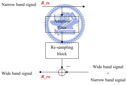
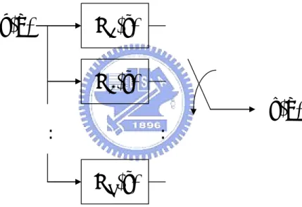
(9) Chapter1. Introduction. Adaptive linear filters have been successfully used in areas such as modeling of unknown systems, linear prediction, adaptive noise canceling, channel equalization systems with high-speed digital communication, echo cancellation, and in many other applications. Applying these adaptive signal processing algorithms to systems with identical transmit rate, say, R_tx samples per sec, and receive rate, say, R_rx samples per sec, is straight forward. However, if a system is with unequal transmit and receive rate, there must exist a rate matching function that accommodates the receiving signal to the filtered signal operating under the same rate for correct data processing. Such mismatched transmit and receive rate scheme can be seen, for example, the echo cancellation filter in the recent applications such as ADSL and VDSL systems. Figure 1.1 shows the conventional rate matching block diagram. Wide / Narrow band R_tx signal Re-sampling block. Adaptive filter. Narrow / Wide band signal R_rx. Wide band signal + Narrow band signal. Figure.1.1 Conventional rate matching structure. R_rx≠R_tx.. There are two situations, one is the higher transmission rate than the receive rate, and 1.

(10) the other is the reverse. For the former, conventional configuration using algorithms such as sub-band adaptive filtering or simply down-sampling the transmitted signal can handle that well. Here, we will not consider that further. But for the latter ( R_rx > R_tx ), the adaptive filter must operate at a higher receive rate which results in an inefficient design. Such configuration shown in figure 1.1 with higher receive rate will increase the length of the filter proportional to R_rx/R_tx and then will quadratic increase the computation complexity of the following adaptive signal processing. For a long system path such as acoustic echo in telephone communication system, such increasing may be inhibited. Alper et al. [1] have proposed an alternative structure shown in Figure 1.2. Narrow band signal. R_tx. Adaptive filter. Re-sampling block. Wide band signal. R_rx. Wide band signal + Narrow band signal. Figure 1.2 Reduced complexity rate matching structure. R_rx > R_tx.. The configuration reverses the order of the re-sampling block and the filter in the conventional structure. In this structure, the adaptive filter is able to operate at the lower transmit rate and thus yields a more efficient design.. 2.

(11) 1.1: Definition of the mismatched ratio. Consider echo cancellation in ADSL system. In this system, the demanding downstream bandwidth is typically a multiple of the bandwidth of the upstream. Particularly, it allows the downstream band to overlap with the upstream band. Suppose the upstream signal is band-limited within f1 and is sampled at a frequency fs1 that is at least larger than twice of f1 to avoid samples aliasing. The downstream signal is band-limited within f2 and is sampled a frequency fs2 which is also a value twice more than f2. Then the mismatched ratio is defined as. Mismatched ratio: M =. f s 2 R_rx = f s1 R_tx. (1.1). For example, suppose the transmit signal and the receive signal are both over-sampled twice, and the upstream and downstream bandwidths are 256 KHz and 1 MHz, respectively, then M = 4.. In this paper, we will consider R_rx is an integer multiple of R_tx. Based on the mismatched rate scheme, we will consider the LMS (Least Mean Square) and the RLS (Recursive Least Square) algorithms in chapter 2. We will also give a convergence analysis of the reduced complexity mismatched rate LMS in chapter 3. Some performance effects introduced by non-ideal re-sampling blocks will be discussed in chapter 4. In chapter 5, simulation will be shown to verify the performance of the algorithms and illustrate our problems in discussion. We conclude this paper in chapter 6. Finally, small capital symbol in bold face denotes a vector, and capital symbol in bold face denotes a matrix in this paper. Transposition of a vector/matrix is denoted as {.}T. Dimension of a symbol will denote beside with lower case if necessary. 3.

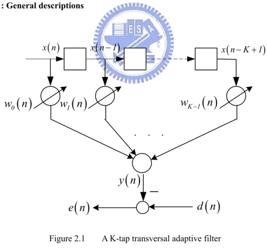
(12) Chapter2. Matched and Mismatched Rate Adaptive Algorithms. Here two popular adaptive algorithms will present, one is LMS, and the other is RLS. In this chapter, we will show how the reduced complexity mismatched rate LMS and RLS is derived. We will first introduce the necessary derivations of conventional LMS and RLS in matched rate environment. The mismatched-rate LMS and RLS with reduced complexity will use their analogies.. 2.1: Matched rate adaptive algorithms. 2.1.1: General descriptions. x ( n − 1). x (n). w0 ( n ). x ( n − K + 1). wK −1 ( n ). w1 ( n ). . . .. y (n). e (n) Figure 2.1. −. d ( n). A K-tap transversal adaptive filter. In Figure 2.1, d(n) is the desired signal generated by a system we are going to identify.. 4.

(13) d(n) can be viewed as a linear combination of the last K samples of the input signal, corrupted by independent zero-mean plant noise v(n). Our aim in this application is to estimate an unknown plant through minimization of the output error e(n) in the mean square sense. For purposes of analysis, we consider the plant to be a transversal FIR filter. Referring to Figure 2.1, the input signal vector at the nth sampling instant is denoted by x ( n ) = ⎡⎣ x ( n ) , ... ,x ( n − K + 1) ⎤⎦ , T. (2.1). and the set of weights of the adaptive transversal filter is denoted by w ( n ) = ⎡⎣ w0 ( n ) , ... ,wK −1 ( n ) ⎤⎦ . T. (2.2). The nth output sample is K −1. y ( n ) = ∑ wi ( n ) x ( n − i ) = w T ( n ) x ( n ) = xT ( n ) w ( n ) .. (2.3). i =0. The input signal vector and the desired response are assumed to be wide-sense stationary. Denoting the desired signal as d(n), the error at the nth time is e ( n ) = d ( n ) − y ( n ) = d ( n ) − w T ( n ) x ( n ) = d ( n ) − xT ( n ) w ( n ) .. (2.4). The square of this error is e 2 ( n ) = d 2 ( n ) − 2d ( n ) x T ( n ) w ( n ) + w T ( n ) x ( n ) x T ( n ) w ( n ) .. (2.5). The mean square error (MSE), ξ , defined as the expected value of e 2 ( n ) , is. ξ ≡ E ⎡⎣ e2 ( n ) ⎤⎦ = E ⎡⎣ d 2 ( n ) ⎤⎦ − 2E ⎡⎣ d ( n ) xT ( n ) ⎤⎦ w ( n ) + w T ( n ) E ⎡⎣ x ( n ) xT ( n ) ⎤⎦ w ( n ). (2.6). = E ⎡⎣ d 2 ( n ) ⎤⎦ − 2p T w ( n ) + w T ( n ) Rw ( n ) , where the cross-correlation vector between the input signal and the desired response is defined as. E ⎡⎣ d ( n ) xT ( n ) ⎤⎦ ≡ p ,. (2.7) 5.

(14) and the input autocorrelation matrix R is defined as. E ⎡⎣ x ( n ) xT ( n ) ⎤⎦ ≡ R = R T .. (2.8). 2.1.2: Wiener filter. The minimum ξ min of ξ can be obtained by differentiating ξ with respect to w ( time index is omitted for clarity ). It can be written in vector gradient form:. ⎡ ∂ξ ∂ξ ∂ξ ⎤ ∇ξ = ⎢ ... ⎥ ∂wK −1 ⎦ ⎣ ∂w0 ∂w1. T. (2.9). where ∇ denotes the gradient operator. By applying matrix differentiations listed in appendix, the gradient vector can be written as:. {. }. ∇ξ = ∇ E ⎡⎣ d 2 ( n ) ⎤⎦ − 2w Tp + w T Rw = ∇ ( −2w Tp ) + ∇ ( w T Rw ) = −2p + ( R + R T ) w .. (2.10). Since R is symmetric, (2.10) can be written as: ∇ξ = 2Rw - 2p .. (2.11). By setting the gradient to zero, we can obtain the well-known Wiener-Hopf equation: Rw o = p ,. (2.12). w = w 0 = R -1p. (2.13). where. is the optimal weight vector known as the Wiener filter tap vector or the Wiener solution. Replacing w ( n ) by w o and Rw o by p in (2.6), we obtain. ξ min = E ⎡⎣ d 2 ( n ) ⎤⎦ − w o Tp = E ⎡⎣ d 2 ( n ) ⎤⎦ − w o T Rw o .. (2.14). 6.

(15) This is the minimum mean-square error that can be achieved by the transversal Wiener filter and is obtained when its tap weights are chosen according to the optimum solution given by (2.13).. Recall (2.6), the MSE ξ can be rearranged as follows:. ξ = w T ( n ) Rw ( n ) − p T w ( n ) − w T ( n ) p + E ⎡⎣ d 2 ( n ) ⎤⎦ . We substitute p with (2.12) and reform the above equation with additional term w oT Rw o , we obtain. ξ = w T ( n ) Rw ( n ) − w oT ( n ) R T w ( n ) − w T ( n ) Rw o + w oT Rw o + E ⎡⎣ d 2 ( n ) ⎤⎦ − w oT Rw o = ( w ( n ) − w o ) R ( w ( n ) − w o ) + E ⎡⎣ d 2 ( n ) ⎤⎦ − w oT Rw o . T. Substitute the right most two terms of the above equation with (2.14), we get. ξ = ξ min + ( w ( n ) − w o ) R ( w ( n ) − w o ) . T. (2.15). We will use (2.15) to study the MSE convergence behavior in chapter 3.. 2.1.3: Steepest-Descent algorithm. Directly find out the Wiener solution of w is not practical. Instead of solving (2.12), the steepest-descent algorithm provides a general scheme that iteratively searches for the minimum point of any convex function. By starting with an initial guess of w , the general iterative update procedure is: w ( n + 1) = w ( n ) − µ∇ξ. (2.16). where µ is a positive scalar step-size, and ξ is the function whose minimum is the goal we are searching for. Substitute (2.11) into (2.16), we derive the steepest-descent update equation:. 7.

(16) w ( n + 1) = w ( n ) − 2 µ ( Rw ( n ) − p ) .. (2.17). The reason why we outline the steepest-descent method here is because one of the important issues in this paper: LMS convergence behavior, will take advantage of its exact description of the stochastic learning curve.. 2.1.4: LMS. LMS is a robust algorithm that is notified by its simplicity of computation and performance of tracking ability. Conventional LMS algorithm is a stochastic implementation of the steepest-descent method. It simply replaces the cost function. ξ = E ⎡⎣e2 ( n ) ⎤⎦ by its instantaneous coarse estimate e 2 ( n ) in (2.16): w ( n + 1) = w ( n ) − µ∇e 2 ( n ) .. (2.18). Noting that the gradient differentiates respect to w , the last term can be written as:. (. ). ∇e 2 ( n ) = 2e ( n ) ∇e ( n ) = 2e ( n ) ∇ d ( n ) − w T ( n ) x ( n ) = −2e ( n ) x ( n ) .. (2.19). Substitute (2.19) into (2.18), the LMS recursive update equation can be written as: w ( n + 1) = w ( n ) + 2 µ e ( n ) x ( n ) .. (2.20). 8.

(17) 2.1.5: RLS. On the goal to obtain the optimum solution, the method of least squares provides a different point of view whose method is primarily based on a deterministic framework, while the LMS provides a statistical framework. In the method of least-squares, at any time instant n > 0, the adaptive filter parameters are calculated so that the cost function n. ζ ( n ) = ∑ λn ( k ) en2 ( k ). (2.21). k =1. is minimized. As RLS is named, it recursively update the adaptive filter tap-weights with feedback estimation error eˆ n −1 ( n ) and the gain vector k ( n ) in the form: ˆ (n) = w ˆ ( n − 1) + k ( n ) eˆ n −1 ( n ) . w. (2.22). The following contents of this sub section will give a brief demonstration of how the update equation holds. Rewrite (2.21) in matrix form:. ζ ( n ) = eT ( n ) Λ ( n ) e ( n ) ,. (2.23). where e ( n ) = ⎡⎣en ( 1) en ( 2 ) L en ( n ) ⎤⎦. T. is a collection of errors, (2.24). and Λ ( n ) = diag ⎡⎣ λ n-1 λ n-2 L 1⎤⎦ , 0 < λ < 1, is the forgetting factor.. There is a corresponding filtered signal y(n) for the desired response d(n) to obtain a specified residue error in the relation of ei ( n ) = d ( i ) − yn ( i ) = d ( i ) − w T ( n ) x ( i ) , i = 1 ~ n .. (2.25) 9.

(18) The corresponding desired response vector d ( n ) = ⎡⎣ d ( 1) d ( 2 ) L d ( n ) ⎤⎦. T. (2.26). and the corresponding filtered signal vector y ( n ) = ⎡⎣ yn ( 1) yn ( 2 ) L yn ( n ) ⎤⎦. T. ˆ ( n) = X ˆ T ( n) w (n) ≡ wT ( n ) X. (2.27). where ˆ ( n ) ≡ ⎡ x ( 1) x ( 2 ) L x ( n ) ⎤ X ⎣ ⎦. (2.28). is the observed input data matrix. The cost function shown in (2.23) can now be written as. ζ ( n ) = d T ( n ) Λ ( n ) d ( n ) − 2θTλ ( n ) w ( n ) + w T ( n ) Ψ λ ( n ) w ( n ) ,. (2.29). where the cross correlation with the desired signal vector ˆ ( n) Λ (n) d ( n) θλ ( n ) = X = x ( n ) d ( n ) + λ x ( n − 1) d ( n − 1) + L. (2.30). = λ θ λ ( n − 1) + x ( n ) d ( n ) and the correlation matrix ˆ (n) Λ (n) X ˆ T (n) Ψλ ( n) = X = x ( n ) x T ( n ) + λ x ( n − 1) x T ( n − 1 ) + L. (2.31). = λ Ψ λ ( n − 1) + x ( n ) x T ( n ) . Differentiate (2.29) with respect to w ( n ) and set the resulting gradient equation to zero, we can write down the normal equation for a linear least-squares filter: ˆ ( n ) = θλ ( n ) Ψλ ( n) w. (2.32). ˆ ( n ) is the estimate of filter tap-weight in the least-squares sense. where w. It follows the least-squares solution:. 10.

(19) ˆ ( n ) = Ψ -1λ ( n ) θ λ ( n ) w = λ Ψ -1λ ( n ) θ λ ( n − 1) + Ψ -1λ ( n ) x ( n ) d ( n ) .. (2.33). Substitute (2.33) into (2.29), the minimum value of ζ ( n ) is obtained as. ζ min ( n ) = d T ( n ) Λ ( n ) d ( n ) − θTλ ( n ) Ψ -1λ ( n ) θ λ ( n ) ˆ (n) . = d T ( n ) Λ ( n ) d ( n ) − θTλ ( n ) w. (2.34). ˆ ( n ) , Ψ -1λ ( n ) In (2.33), it is clear that if we want to find the optimum solution of w. must be solved. Using (2.31) and the matrix inverse lemma shown in appendix B, we have. λ −2 Ψ -1λ ( n − 1) x ( n ) xT ( n ) Ψ -1λ ( n − 1) Ψ ( n ) = λ Ψ ( n − 1) − 1 + λ −1xT ( n ) Ψ -1λ ( n − 1) x ( n ) -1 λ. −1. -1 λ. ≡ λ ⎡⎣ Ψ −1. -1 λ. (2.35). ( n − 1) − k ( n ) x ( n ) Ψ ( n − 1)⎤⎦ , T. -1 λ. where k (n) ≡. λ −1Ψ -1λ ( n − 1) x ( n ). 1 + λ −1x T ( n ) Ψ -1λ ( n − 1) x ( n ). .. (2.36). Write (2.36) out, we have. k ( n ) = λ −1 ⎡⎣ Ψ -1λ ( n − 1) − k ( n ) xT ( n ) Ψ -1λ ( n − 1) ⎤⎦ x ( n ) .. (2.37). Substitute (2.35) into (2.37), we obtain k ( n ) = Ψ -1λ ( n ) x ( n ) .. (2.38). Rewrite (2.33) with (2.38), we have ˆ ( n ) = λ Ψ -1λ ( n ) θ λ ( n − 1) + k ( n ) d ( n ) . w. (2.39). Now replace Ψ -1λ ( n ) with the recursion derived in (2.35), we get. 11.

(20) ˆ ( n ) = Ψ -1λ ( n − 1) θ λ ( n − 1) + k ( n ) x T ( n ) Ψ -1λ ( n − 1) θ λ ( n − 1) + k ( n ) d ( n ) w ˆ ( n − 1) − k ( n ) x T ( n ) w ˆ ( n − 1) + k ( n ) d ( n ) =w. (. ˆ ( n − 1) + k ( n ) d ( n ) − x T ( n ) w ˆ ( n − 1) =w. ). (2.40). ˆ ( n − 1) + k ( n ) en −1 ( n ) . ≡w. Here the estimation error en −1 ( n ) is defined as: ˆ ( n − 1) , determined by past weights and current input. (2.41) en −1 ( n ) = d ( n ) − xT ( n ) w. In summary, the standard RLS update procedures is as follows: 1.. Update the gain vector: (2.36). u ( n ) = Ψ -1λ ( n − 1) x ( n ) , denk = λ + xT ( n ) u ( n ) ,. k (n) = 2.. u (n) denk. .. Update the estimation error en −1 ( n ) : (2.41) ˆ ( n − 1) . en −1 ( n ) = d ( n ) − xT ( n ) w. 3.. ˆ ( n ) : (2.40) Update the tap weights w ˆ (n) = w ˆ ( n − 1) + k ( n ) en −1 ( n ) . w. 4.. Update Ψ -1λ ( n ) : (2.35). Ψ -1λ ( n ) = λ −1 ⎡⎣ Ψ -1λ ( n − 1) − k ( n ) xT ( n ) Ψ -1λ ( n − 1) ⎤⎦. {. }. = Tri λ −1 ⎡⎣ Ψ -1λ ( n − 1) − k ( n ) u T ( n ) ⎤⎦. .. The last equation has two purposes. One is to save the computation and the other is to stabilize the RLS convergence in implementation. Tri{} is the operator that extracting the lower or upper part of the operating matrix and copies them to the either side except the diagonal.. 12.

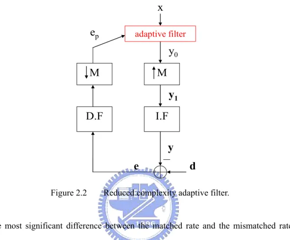
(21) 2.2: Mismatched-rate adaptive algorithms with reduced complexity. x ep. adaptive filter. y0 M. M y1. D.F. I.F y e. Figure 2.2. d. Reduced complexity adaptive filter.. The most significant difference between the matched rate and the mismatched rate system is that the number of the received desired signal samples in the mismatched rate system is M (or even larger) times more than that in the matched rate system. To cooperate with the characteristics of the received signal d, the identifying filtered signal y must be designed, at least, to match d in number. On the other hand, the reduced complexity structure is meaningfully proposed because the structure is using conventional adaptive algorithms even though it is in an environment that gives an increasing amount of data. In figure 2.2, the reduced complexity structure shows its clever collaboration. “IF” and “DF” denote the interpolation filter and the decimation filter respectively. The structure uses up-sample block to treat the filter output to match the number of received signal, and uses down-sample block to treat the filter input to maintain the low complexity. Notice that if extra wide band noise was added. 13.

(22) such that the signal d is not a narrow band signal, the down-sample block may give a mechanism that suppresses the disturbance and makes the filter input less noisy.. 2.2.1: General descriptions. In order to derive the reduced complexity adaptive filter update rule, we now write each necessary component out. Starts from the output of the adaptive filter y0 , all necessary components following the arrow direction in figure 2.2 will be shown step by step. The operating function of each component will be also described in detail. Let NI and ND denote the order of the interpolation and the decimation filter. We start from y0 , a simply K-tap linear transversal filter output: K −1. y0 ( n ) = ∑ wi ( n ) x ( n − i ) = w T ( n ) x ( n ) = xT ( n ) w ( n ) .. (2.42). i =0. In the initial state, the reduced complexity adaptive filter starts to train until it collects L filtered outputs, where L is a number we will show later. In other words, the filter starts to train when n = L, and at the same time, y0 ( 1) ,L , y0 ( L ) have already collected. Reform the filtered outputs into a vector form ⎡ K −1 ⎤ wi ( n ) x ( n − i ) ⎥ ∑ ⎢ ⎡ y0 ( n ) ⎤ i =0 ⎥ ⎢ ⎥ ⎢ y0 ( n) = ⎢ M M = ⎢ ⎥ ⎥ ⎥ ⎢ y ( n − L + 1) ⎥ ⎢ K −1 ⎣ 0 ⎦ ⎢ ∑ wi ( n ) x ( n − L + 1 − i ) ⎥ ⎢⎣ i =0 ⎥⎦ ≡ X (n) w (n) ,. (2.43). where the input data are organized in a Hankel matrix form as. X ( n ) L× K. ⎡ x (n) x ( n − 1) ⎢ x ( n − 2) ⎢ x ( n − 1) ≡⎢ M M ⎢ ⎢ x ( n − L + 1) x ( n − L ) ⎣. L L M L. x ( n − K + 1) ⎤ ⎥ x (n − K ) ⎥ ⎥. M ⎥ x ( n − L − K + 2 ) ⎦⎥. (2.44). 14.

(23) From (2.44), we can see that the adaptive filter pays L+K-1 latencies before starting to train. Passing y0(n) through an M times zero insertion up-sampler, we write the resulting vector y1(n) in matrix form: y1 ( n ) ≡ Ω y 0 ( n ) = Ω X ( n ) w ( n ) ,. (2.45). where Ω is a zero insertion matrix. For example, if M = 2, Ω can be written as. Ω J ×L. ⎡ ⎢ ⎢ ⎢ ⎢ ⎢ =⎢ ⎢ ⎢ ⎢ ⎢ ⎢ ⎢ ⎣. 100L 000L 010L 000L M 000L 000L 000L 000L. 0⎤ 0 ⎥⎥ 0⎥ ⎥ 0⎥ M⎥ ⎥ 0 1 0⎥ 0 0 0⎥ ⎥ 0 0 1⎥ 0 0 0 ⎥⎦. where J = ND+NI+M-2, which is a number designed to fit the following matrix operation. In view of Ω , we can now determine that L = ceil( J/M ). Next we determine the signal y ( n ) that passes y 1 ( n ) through the interpolation filter as: y ( n ) ≡ F y1 ( n ) = F Ω X ( n ) w ( n ) ,. (2.46). where F is the convolution matrix with dimension ND+M-1 by J. Suppose the interpolation filter coefficients are f1 L f N I , F can be written as: L f N I −1 f N I 0 ⎡ f1 f 2 ⎢ f1 f 2 L f N I −1 f N I ⎢ F=⎢ O O ⎢ f1 f 2 L f N I −1 f N I ⎢⎣ 0. ⎤ ⎥ ⎥ ⎥. ⎥ ⎥⎦. (2.47). 15.

(24) In (2.46), it shows that there are ND+M-1 samples to match the desired response. Actually, only first M samples are needed and the rest of them are not in use at present. One may question that if the rest of samples are useless, why do we need to compute them? This answer lies in whether we use the decimation filter or not. If we neglect the decimation filter, the dimension of y ( n ) is M and no redundant computations will be needed. However, in specific application such as echo cancellation in ADSL, the downlink high frequency components will exist in the operating band of the received signal and is recognized as a disturbance for echo identification (notice that we only want the signal generated by the echo path in the received signal for echo cancellation). If there is no barrier such as the low pass decimation filter, the feedback error will be no longer clean and the performance will consequently decay. Return to our discussion, the error vector e ( n ) with dimension ND+M-1 is e ( n) = d (n) − y ( n) .. Suppose the decimation filter coefficients are g1 L g N D , and one of the first M phases, say, phase p, is selected to do the decimation. Then we can write the down sampled error ep(n), a scalar, as: e p ( n ) = gpe ( n ) ,. (2.48). where the combined effect of decimation filter and the decimator can be written as: g p = ⎡⎣ zeros ( p − 1) g1 L g N D zeros ( M − p ) ⎤⎦ , 1 ≤ p ≤ M .. (2.49). Here “zeros(k)” means there are k zeros line in a row, k ≥ 0 . Finally, we combine the effects of the up-sample block and the down-sample block into a vector hp , dimension 1 by L: hp = gp F Ω ,. (2.50) 16.

(25) where p is the decimator chosen phase. The study of the combined effect hp is one of the major topics in this paper.. 2.2.2: LMS. The cost function here is e 2p ( n ) . By using (2.46), (2.48) and (2.50), the square of the down sampled error can be written as: e2p ( n ) = ⎡⎣g p e ( n ) ⎤⎦ = ⎡⎣g p d ( n ) − g p y ( n ) ⎤⎦ 2. = ⎡⎣g p d ( n ) − g p F Ω X ( n ) w ( n ) ⎤⎦ = ⎡⎣g p d ( n ) − hp X ( n ) w ( n ) ⎤⎦. 2. 2. 2. (2.51). = ⎡⎣d T ( n ) g pT − w T ( n ) XT ( n ) hpT ⎤⎦ . 2. Using the analogies of (2.18), differentiate (2.51) with respect to w , we get ∇e2p ( n ) = 2e p ( n ) ∇e p ( n ) = −2e p ( n ) XT ( n ) hpT .. (2.52). Substitute (2.52) into (2.18), we have the LMS update rule: w ( n + 1) = w ( n ) + 2 µ e p ( n ) XT ( n ) hpT .. (2.53). Notice that since hp is determined once the IF and DF are determined, rather than calculating the whole hp X ( n ) , one may use the shifting property of X ( n ) such that only the latest L data have to be processed during each update.. 17.

(26) 2.2.2.1: Simplified version. Since both the interpolation filter and the decimation filter are low pass filters, the combined effect hp can be designed to have an impulse response similar to sinc ˆ set the dominant function with one dominant coefficient. The simplified version h p coefficient of hp one and set the rest of them zeros. Now we can get ˆ X ( n ) = ⎡ x ( n − d ) x ( n − d − 1) L x ( n − d − K − 1) ⎤ , h p ⎣ ⎦ where d is the index of the largest element of hp . Then the update rule of LMS can be written as w ( n + 1) = w ( n ) + 2 µ e p ( n ) x ( n − d ) .. (2.54). Observe (2.54), it is just the same as the conventional LMS update equation in (2.20).. Compared to the original LMS, the simplified version replaces the color factor hp ˆ . Before the original LMS updates, it has to process the input with a delta function h p data by the combined effect hp. As we shall discuss in chapter 4, the combined effect will become a color factor of the input data if the distortion exists within the up-sample and down-sample blocks. The simplified version can avoid such color effect of the input data and hence the convergence speed will be faster than the original LMS in most of the cases. Performance comparison between the reduced complexity adaptive algorithm and its simplified version will be shown in section 5.1.. 18.

(27) 2.2.3: RLS. Reduced complexity RLS algorithm is similar to the conventional RLS algorithm by simply modifies the input data sequence. In this paper, we call this reduced complexity RLS for mismatched rate system by “vector input” RLS. Recall (2.44), the Hankel input data matrix can be written as X ( n ) L×K = ⎡⎣ x ( n ) x ( n − 1) L. x ( n − K + 1) ⎤⎦ ,. x ( n ) L×1 = ⎡⎣ x ( n ) x ( n − 1) L. x ( n − L + 1) ⎤⎦ .. where T. Then the “vector input” RLS data sequence has the form: h p X ( n ) = ⎡⎣hp x ( n ) h p x ( n − 1) L. hp x ( n − K + 1) ⎤⎦. 1× K. .. (2.55). The difference between the “vector input” RLS and the conventional RLS is that the update of the “vector input” RLS data sequence needs to compute h p x ( n ) , which requires L multiplications and L-1 additions, and the conventional RLS needs just a shift. The “vector input” RLS is named because it requires a vector x ( n ) with length L to compute the latest input data feasible for updating the mismatched rate RLS system. The “vector input” RLS modifies the conventional RLS by its input from x ( n ) to h p x ( n ) , so the cross correlation vector becomes θ λ ( n ) = λ θ λ ( n − 1) + X ( n ) h pT d ( n ) ,. (2.56). and the correlation matrix becomes Ψ λ ( n ) = λ Ψ λ ( n − 1) + X T ( n ) hpT h p X ( n ) .. (2.57). 19.

(28) By simply substitute x ( n ) in conventional RLS with ⎡⎣hp X ( n ) ⎤⎦ , we summarize T. the reduced complexity mismatched rate RLS as follows. 1.. Update the gain vector: u ( n ) = Ψ -1λ ( n − 1) XT ( n ) hpT , denk = λ + hp X ( n ) u ( n ) , k (n) =. 2.. u (n) denk. .. Update the filtering error e p ( n ) : y ( n) = F Ω X ( n) w ( n) e p ( n ) = g p ⎡⎣d ( n ) − y ( n ) ⎤⎦ , note that h = g p F Ω.. 3.. Update the tap weights w ( n ) : w ( n ) = w ( n − 1) + k ( n ) e p ( n ) .. 4.. Update Ψ -1λ ( n ) :. {. }. Ψ -1λ ( n ) = Tri λ −1 ⎡⎣ Ψ -1λ ( n − 1) − k ( n ) u T ( n ) ⎤⎦ .. RLS simplified version can use the same update methods listed above by replacing ˆ , where h ˆ is exactly the same described in section 2.2.2.1. hp by h p p. Applying conventional RLS into this structure is straight forward, but there are still something special we have to take care with, we point them out in the next sub-section.. 2.2.3.1: Initialization problems. Two kinds of initialization scheme we will demonstrate in this paper, one happens in. 20.

(29) the beginning of the training, and the other may happen in the midway. For the initialization in the beginning of training, there are several kinds of popular data matrix windowing [2]. Here we will use two of them. One is pre-windowing, and the other is covariance windowing. Using the pre-windowing for the data matrix is to start the input data sequence from all zero and no latencies are paid. Using covariance windowing for the data matrix is to fill the input data sequence with only data and we have to pay L-K+1 latencies for full-filling the data matrix. In this paper, we often use the covariance windowing. The pre-windowing is used in some special cases such as re-initialization problem. In the reduced complexity structure, the performance of the pre-windowing version is a little worse than the covariance windowing version which pays latencies for initializing the sequence with hpX(n). We will see the demonstrations in section 5.2.1.. The initialization problem can apply not only in the beginning of the training, but also in the midway. In real time applications, the limited memory size in DSP and the power consumption may be big factors for continuous adaptation of RLS. One of the straight forward solutions is to stop adaptation for a while and wait until the previous computations complete offline. To maintain the performance under this stagnant adaptation, the re-initialization is developed for this RLS computation-relaxed case. The other application for the RLS re-initialization is the adaptation for time varying channels. If the RLS adaptive filter has finished training for a channel before it changes, we may periodically modify the existing RLS parameters to fit the current channel condition. For such modification, re-initialization may be used to maintain the tracking performance. We will not consider this case in our simulation experiment. For the computation-relaxed problems, the performance of the transient state (convergence) and the steady state (tracking) of the adaptive filter are both under 21.

(30) challenges due to un-consistent adaptations. We can assert that the performance will degradation if the algorithm has no modification for this situation. In section 5.2.2, we will demonstrate the re-initialization phenomenon.. 2.3: Remarks. The adaptive filters demonstrated in section 2.2 are all designed based on minimizing e 2p ( n ) no matter in its statistical property or in exact value. Because of the filter. inputs hpX(n) and e 2p ( n ) are all operating in a lower rate, it is natural to see that the complexity of the mismatched rate system adaptation is similar to that of the conventional adaptive algorithm. Table 2.1 shows the number of multiplications at each update iteration applying different architectures for these algorithms.. Reduced complexity. LMS. Simplified LMS. RLS. (L+1)(K+ND+M). (L+1)(K+ND+M)-L. 2K2+(L+2)K. structure. Fig.1.2. +(L+1)(ND+M-1)+L. Conventional. ~M2 times more. structure. Fig.1.1. than the above.. “. ~M2 times more than the above.. Table 2.1: Number of multiplications in update equations.. At last, the performance comparison between LMS and RLS by inputting the same sequence (input data and desired responses) will also be shown in section 5.3.. 22.

(31) Chapter3. Convergence Behavior of mismatched Rate LMS. In this chapter, the convergence behavior of the reduced complexity mismatched rate LMS algorithm will be addressed. Besides its MSE learning curve, we will also give a prediction of its convergence speed and optimum convergence bound. In this chapter, we will first show some basic concepts about how conventional LMS is modeled for its convergence behavior. Some tools such as the steepest-descent method and Wiener-Hopf equation introduced in section 2.1 will be used to analyze the LMS convergence. Then the reduced complexity algorithm will be studied.. 3.1: Matched rate LMS convergence behavior. Before entering the LMS convergence section, we first introduce the convergence analysis of the steepest-descent method, which will give us some deterministic insights of the convergence behavior of such stochastic adaptive algorithms. The convergence analysis is following the derivations listed in [4], [5].. 3.1.1: The steepest-descent method. The steepest-descent method provides us a deterministic way to derive some necessary convergence indices such as the time constants that we will use later. To study the convergence behavior of stochastic adaptive algorithm, we start from analyzing their MSE (mean square error).. 23.

(32) Recall (2.15), the learning curve can be written as. ξ ( n ) = ξ min + ( w ( n ) − w o ) R ( w ( n ) − w o ) . T. Note that the learning curve is defined as the MSE ξ versus the time index n. This formula shows that the convergence goes to a steady state once its filter tap-weights approach w0, at that moment, ξ ≅ ξ min . Here, given the stationary signals x(n) and d(n), the optimum tap-weight vector w0, can be determined according to the. Wiener-Hopf equation listed in (2.13). However, with only (2.15), there is not enough information to give further insights such as convergence speed and some other interesting issues. The right-hand term of (2.15) can be expanded. ξ ( n ) = ξ min + ( w ( n ) − w o ) QΛQT ( w ( n ) − w o ) . T. (3.1). Here we use the unitary similarity decomposition property of a symmetric matrix, R is decomposed as R = QΛQ T ,. (3.2). where Λ is a diagonal matrix consisting of the eigenvalues λ0 ,λ1 ,L ,λK −1 of R and the columns of Q contain the corresponding orthonormal eigenvectors. Define the weight-error vector v(n) as v ( n) = w ( n ) − wo ,. (3.3). we can rewrite (3.1) as. ξ ( n ) = ξ min + v T ( n ) QΛQ T v ( n ) .. (3.4). Now define the transformed weight-error vector v’(n) as v’(n) = QT v(n), we can get. ξ ( n ) = ξ min + v ' ( n ) Λv ' ( n ) T. K −1. = ξ min + ∑ λi v'i2 ( n ) . (scalar form). (3.5). i =0. To derive the transformed weight-error v’(n) for the steepest-descent method, its 24.

(33) update equation (2.16) is rewritten as w ( n + 1) = ( I − 2 µ R ) w ( n ) + 2 µ p .. (3.6). where I is the K by K identity matrix. Subtract w0 from both sides of (3.6) and rearrange the result to obtain w ( n + 1) − w o = ( I − 2 µ R ) ( w ( n ) − w o ). (3.7). here we replace p by (2.12). Substitute into (3.7), we obtain v ( n + 1) = ( I − 2 µ R ) v ( n ) .. (3.8). Substituting (3.8) into (3.7) and replacing I with QQT, rewrite (3.8) as. (. ). v ( n + 1) = QQ T − 2 µ QΛQ T v ( n ) = Q ( I − 2µ Λ ) Q v ( n) . T. (3.9). Then transform v(n) to v’(n) by pre-multiplying (3.9) by QT, the recursive equation (3.9) is now reformed as v ' ( n + 1) = ( I − 2 µ Λ ) v ' ( n ) .. (3.10). The vector recursion (3.10) can be separated into the scalar recursive equations vi ' ( n + 1) = ( 1 − 2 µλi ) vi ' ( n ) , for i = 0,1,...,K − 1 ,. (3.11). where vi ' ( n ) is the ith element of the vector v ' ( n ) . Starting with a set of initial values v0 ' ( 0 ) ,v1 ' ( 0 ) ,L ,vK −1 ' ( 0 ) and iterating n times, the scalar recursion can be written as vi ' ( n ) = ( 1 − 2 µλi ) vi ' ( 0 ) , for i = 0,1,...,K − 1 . n. (3.12). Substitute (3.12) into (3.5), we now derive the learning behavior of the steepest descent method:. 25.

(34) K −1. ξ ( n ) = ξ min + ∑ λi v'i2 ( n ) i =0. K −1. (3.13). = ξ min + ∑ λi ( 1 − 2 µλi ) v' ( 0 ) . 2n. i =0. 2 i. If µ is property selected, then (3.13) converges to ξ min as n increases. In (3.13), the MSE is consisted of the sum of K exponentially decaying terms each of which corresponds to one of the modes of convergence of the algorithm.. 3.1.2: Eigenvalue spread. Each exponential term in (3.13) can be characterized by a time constant which is obtained as follows. Let. (1 − 2 µλi ). 2n. = e− n / τ i. (3.14). and define τ i as the time constant associated with the exponential term ( 1 − 2 µλi ) . 2n. Solving (3.14) for τ i , we get. τi =. −1 . 2 ln ( 1 − 2 µλi ). (3.15). When 2 µλi = 1 , ln ( 1 − 2 µλi ) ≅ −2 µλi . Substitute this in (3.15), we obtain. τi ≅. 1 4 µλi. .. (3.16). We can see in (3.16) that large eigenvalue λi causes small time constant, so there is a faster convergence speed for the tap-weight coefficient wi , i = 0,1,...,K − 1 . However, the MSE convergence is determined by the whole tap-weight coefficients, a single time constant cannot thoroughly govern the convergence speed. We observe this situation in (3.12). The necessary and sufficient condition of convergence is. 26.

(35) ( I − 2µ Λ ). or. n. → 0, as n → ∞ ,. ⎡( 1 − 2 µλ0 )n ⎤ L 0 0 ⎢ ⎥ n ⎢ ⎥ M 0 (1 − 2 µλ0 ) ⎢ ⎥ → 0, as n → ∞ . (3.17) M O M ⎢ ⎥ ⎢ n⎥ L L 0 (1 − 2 µλ0 ) ⎥⎦ ⎢⎣. So that if the maximum of these eigenvalues, say, λmax , is large, and others are relatively small, the convergence speed will still be delayed by the other eigenvalues. Hence, the eigenvalue spread provides a good merit for the convergence speed. It is defined as Eigenvalue spread χ ( R ) =. λmax . λmin. (3.18). Eigenvalue spread is a condition number of matrix R. R is ill-conditioned if the eigenvalue spread is large. Some analysis [4], [5] have shown that the eigenvalue spread is relative to the spectrum of the input data sequence. The eigenvalue spread is bounded by the ratio of the maximum and the minimum of the input data spectrum and is approximately the same when the sequence length is long enough. In this observation, it is natural to conclude that the input data with a flatter spectrum has a smaller eigenvalue spread, and accordingly the adaptive filter will have a faster convergence speed.. 27.

(36) 3.1.3: LMS convergence behavior. Assume that the input signal x(n) and the desired response d(n) are zero-mean stationary process and are all jointly Gaussain-distributed random variables. And at time n, the tap-weight vector w(n) is independent of the input vector x(n) and the desired response d(n). Based on these assumptions, we start to analyze the mean square error E[e2(n)] of the conventional LMS algorithm. Such analysis can be seen in [4], [5]. Recall (2.20), the update equation of LMS, subtracting w0 from both sides, we obtain: v ( n + 1) = v ( n ) + 2 µ e ( n ) x ( n ) .. (3.19). where v(n) = w(n) - w0 is the weight-error vector. Also notes that. e ( n ) = d ( n ) − y ( n ) = d ( n ) − w T ( n ) x ( n ) = d ( n ) − xT ( n ) w ( n ) = d ( n ) − xT ( n ) w 0 − xT ( n ) ( w ( n ) − w 0 ). (3.20). = eo ( n ) − xT ( n ) v ( n ). where eo ( n ) = d ( n ) − x T ( n ) w o. (3.21). is the estimation error when the filter tap weights are optimum. Squaring both sides of (3.20) and taking the expectation on both sides, we obtain 2 e ( n ) = E ⎡⎣eo2 ( n ) ⎤⎦ + E ⎡( v T ( n ) x ( n ) ) ⎤ − 2E ⎡⎣ eo2 ( n ) v T ( n ) x ( n ) ⎤⎦ . ⎢⎣ ⎥⎦. (3.22). Noting that v T ( n ) x ( n ) = xT ( n ) v ( n ) and using the independent assumption between the tap weights and the input signal, the second term on the right-hand side of (3.22) can be expanded as. 28.

(37) (. ). 2 E ⎡ v T ( n ) x ( n ) ⎤ = E ⎡⎣ v T ( n ) x ( n ) xT ( n ) v ( n ) ⎤⎦ ⎥⎦ ⎣⎢ = E ⎡⎣ v T ( n ) E ⎡⎣ x ( n ) xT ( n ) ⎤⎦ v ( n ) ⎤⎦ = E ⎡⎣ v T ( n ) R v ( n ) ⎤⎦ .. (3.23). Noting that v T ( n ) x ( n ) is a scalar, rewrite (3.5) as. (. {. ). }. 2 E ⎡ v T ( n ) x ( n ) ⎤ = tr E ⎡⎣ v T ( n ) x ( n ) x T ( n ) v ( n ) ⎤⎦ ⎢⎣ ⎥⎦. {. }. = tr E ⎡⎣ v T ( n ) E ⎡⎣ x ( n ) x T ( n ) ⎤⎦ v ( n ) ⎤⎦. { } = E ⎡⎣tr { v ( n ) v ( n ) R }⎤⎦ = E ⎡⎣tr v T ( n ) R v ( n ) ⎤⎦. (3.24). T. {. }. = tr E ⎡⎣ v ( n ) v T ( n ) ⎤⎦ R .. Here we use the matrix trace property: tr {AB} = tr {BA} for facilitating the term exchanging operation. Define the correlation matrix of the weight-error vector v(n) as K ( n ) ≡ E ⎡⎣ v ( n ) v T ( n ) ⎤⎦ ,. (3.25). the above result reduces (3.6) to. (. ). 2 E ⎡ v T ( n ) x ( n ) ⎤ = tr {K ( n ) R} . ⎢⎣ ⎥⎦. (3.26). Using the independent assumption and noting that eo(n) is a scalar, the last term on the right-hand side of (3.22) can be written as E ⎡⎣eo2 ( n ) v T ( n ) x ( n ) ⎤⎦ = E ⎡⎣ v T ( n ) ⎤⎦ E ⎡⎣ x ( n ) eo2 ( n )⎤⎦ = 0 ,. (3.27). Using (3.26) and (3.27) in (3.22), we obtain. ξ = E ⎡⎣ e2 ( n ) ⎤⎦ = ξ min + tr {K ( n ) R} .. (3.28). where ξ min = E ⎡⎣eo2 ( n ) ⎤⎦ , that is, the minimum mean-square error (MSE) at the filter output. (3.28) can be written in a form that is more convenient for future analysis. Recall (3.2), 29.

(38) by decomposing R and using the matrix trace term commute rule, we obtain. ξ = E ⎡⎣e2 ( n ) ⎤⎦ = ξ min + tr {K ' ( n ) Λ} .. (3.29). where K ' ( n ) = Q T K ( n ) Q . Furthermore, using (3.25) and definition v’(n) = QT v(n) from section 3.1, we find that T K ' ( n ) ≡ E ⎡ v' ( n ) v' ( n ) ⎤ . ⎣ ⎦. (3.30). Noting that Λ is a diagonal matrix composed of eigenvalues of R, (3.29) can be expanded as K −1. ξ = E ⎡⎣ e2 ( n ) ⎤⎦ = ξ min + ∑ λi kii' ( n ). (3.31). i =0. where kij' ( n ) is the ijth element of the matrix K ' ( n ) . The LMS on average follows the same trajectory as the steepest-descent method [4]. Despites the noisy variation of the filter tap weight, the learning curve of the LMS matches closely the theoretical results of the steepest-descent method. To this end, (3.13) is applicable and the time constant. τi ≅. 1 4 µλi. (3.32). can be used for predicting the transient behavior of the LMS algorithm. Consequently, the eigenvalue spread introduced in section 3.1.1.1, can be used to indicate the convergence speed of the LMS algorithm given an input data autocorrelation matrix.. 30.

(39) 3.2: Mismatched rate LMS convergence behavior. x ep. LMS. M. M. D.F. I.F y e. Figure. 3.1. d. Reduced complexity mismatched rate LMS filter.. Let the down sampled desired signal dp(n) as d p ( n ) = gpd ( n ) , 1 ≤ p ≤ M. (3.33). where g p = ⎡⎣ zeros ( p − 1) g1 L g N D zeros ( M − p ) ⎤⎦ , 1 ≤ p ≤ M . Rewrite the down sampled error (2.51) as 2 2 E ⎡⎣e 2p ⎤⎦ = E ⎡( g p d − g p y ) ⎤ = E ⎡( d p − hp Xw ) ⎤ ⎢⎣ ⎥⎦ ⎢⎣ ⎥⎦. = E ⎡⎣ d p2 ⎤⎦ − w T E ⎡⎣ XThpT d p ⎤⎦ − E ⎡⎣ d p hp X ⎤⎦ w + w T E ⎡⎣ XThpThp X ⎤⎦ w .. (3.34). Define the cross correlation vector of the mismatched rate system as E ⎣⎡ XT ( n ) hpT d p ⎦⎤ ≡ qp. (3.35). and the autocorrelation matrix as E ⎡⎣ XT ( n ) hpThp X ( n ) ⎤⎦ ≡ R p = R pT .. (3.36). Substitute (3.35) and (3.36) into (3.34), we can get: 31.

(40) E ⎡⎣e 2p ⎤⎦ = E ⎡⎣ d p2 ⎤⎦ − 2w Tqp + w T R p w , 1 ≤ p ≤ M .. (3.37). Using the Wiener-Hopf equation (2.12), the optimum tap-weight is w o,p = R p-1qp .. (3.38). With this optimum tap-weight, the convergence of this structure has an optimum to approach. Similar to (2.15), (3.37) can be written as E ⎡⎣e 2p ⎤⎦ = ξ min, p + ( w − w o, p ) R p ( w − w o, p ) , 1 ≤ p ≤ M . T. (3.39). where ξ min, p is the minimum mean square error of the mismatched rate LMS training system and can be written as. ξ min, p = E ⎡⎣ d p2 ⎤⎦ − qpT R p-1 qp , 1 ≤ p ≤ M .. (3.40). One must notice that the lower case of “p” besides these symbols. It represents which phase of the error vector e(n) is chosen and the convergence of MSE and its MMSE are all relative to it. The effects of choosing different phase (performance, convergence speed) will be discussed in the next chapter.. Similar to the LMS convergence derivation, by replacing the autocorrelation matrix with Rp, we can obtain the behavior of the mean square value of e p as:. ξ p ( n ) = ξ min, p + tr {K p ( n ) R p } , 1 ≤ p ≤ M .. (3.41). Here we define vp(n) = w(n) – wo,p is the weight-error vector with respect to phase p, and define the correlation matrix of the weight-error vector vp(n) as K p ( n ) ≡ E ⎡⎣ v p ( n ) v pT ( n ) ⎤⎦ .. (3.42). R p = Qp Λ p QpT ,. (3.43). Decompose Rp as:. 32.

(41) where Λ p is a diagonal matrix consisting of the eigenvalues λ0 ,p , λ1,p L , λK −1,p of Rp and the columns of Qp contain the corresponding orthonormal eigenvectors.. Using (3.43), we can write (3.42) as. ξ p ( n ) = ξ min, p + tr {K p ' ( n ) Λ p } , 1 ≤ p ≤ M. (3.44). Notice that v p ' ( n ) = QpT v p ( n ) , then T K p ' ( n ) = E ⎡ vp ' ( n ) vp ' ( n ) ⎤ ⎣ ⎦. T = Qp K p ( n ) Qp. (3.45). (3.44) can be also written in scalar form as K −1. ξ p ( n ) = E ⎡⎣e 2p ( n ) ⎤⎦ = ξ min, p + ∑ λi ,p kii' , p ( n ) , 1 ≤ p ≤ M. (3.46). i =0. where kij' , p ( n ) is the ijth element of the matrix K p ' ( n ) .. The above can be seen as the convergence behavior of the mismatched rate system, but for problems such as echo cancellation, equation (3.46) may not be able to provide us enough information about the echo attenuation level. For such problems, the “true error” we concern is the input of the down-sampling block, the error vector e(n). Unlike ep(n), it only gives a partial information, the value of e(n) (norm) is the direct result of the interpolated filtered signal and the received signal. It gives us a more complete information about the system identification. Here, we take e(n) as our performance index and the rest of this chapter will be devoted to derive its convergence behavior.. 2 Now, we focus on the derivation of E ⎡⎢ e ( n ) ⎤⎥ . ⎣ ⎦. Recall (2.48) and (2.49), we collect all ep(n)s,. p = 1~M in a vector ep(n). 33.

(42) ⎡ e1 ( n ) ⎤ ⎢ ⎥ ep ( n ) = ⎢ M ⎥ = Ge ( n ) ⎢e ( n )⎥ ⎣ M ⎦. (3.47). where. G M ×( N D + M −1). L g N D−1 g N D 0 ⎤ ⎡ g1 g 2 ⎢ ⎥ O O =⎢ ⎥ ⎢0 L g1 g 2 g N D−1 g N D ⎥⎦ ⎣. (3.48). is a convolution matrix filled with coefficients of the decimation filter. In (3.47), we can see that e ( n ) = G -1ep ( n ) if G-1 exits.. (3.49). But as we can see in (3.48), the dimension of the convolution matrix makes the existence of G-1 impossible. If we force a matrix A such that AG = I, we may find the left inverse matrix of G. However, to simplify this derivation and make it intuitive, we will not focus on the derivation of the left inverse matrix of G. Instead, we will study the convergence of each sampling phase of e(n) individually.. 3.2.1: Convergence analysis of each phase. x. M Figure. 3.2. IF. DF. M. x’. Combination of the interpolator and the decimator.. Observing the path through the up-sampling and down-sampling block, a typical combination of the interpolator and the decimator can be plotted as shown in figure. 34.

(43) 3.2. In this figure, both the cut-off frequencies of the interpolation filter and the decimation filter are π / M . Such combination can be simplified by removing one of the low pass filters as we have known in the digital signal processing text book. The motivation of the following structure which help us to analyze the convergence of e(n) comes from this simplification.. x ep. LMS. M. M. I.F y, dim = M e, dim = M Figure. 3.3. d, dim = M. A convergence analysis convenient structure.. The structure in figure 3.3 neglects the decimation filter. In this simplified structure, the convolution matrix shown in (3.48) is now simplified to an identity matrix with dimension M, and (3.49) now can be written as e ( n ) = ep ( n ) , 1 ≤ p ≤ M .. (3.50). Hence, we can get 2 E ⎡⎢ e ( n ) ⎤⎥ = E ⎡⎣eT ( n ) e ( n ) ⎤⎦ = E ⎡⎣epT ( n ) ep ( n ) ⎤⎦ ⎣ ⎦ M. = ∑ E ⎡⎣e2p ( n ) ⎤⎦ .. (3.51). p =1. Finally, substitute (3.46) into (3.51), the desired learning behavior can be written as:. 35.

(44) M. 2 E ⎡⎢ e ( n ) ⎤⎥ = ∑ E ⎡⎣e2p ( n ) ⎤⎦ ⎣ ⎦ p =1 M. M K −1. p =1. p =1 i =0. = ∑ ξ min, p + ∑ ∑ λ k. ' i , p ii , p. (n) .. (3.52). The analysis of the simplified LMS can be obtained using the same way. Modifying the autocorrelation matrix Rp with. ˆ = E ⎡ XT ( n ) h ˆ Th ˆ ⎤ R p p p X ( n )⎦ , 1 ≤ p ≤ M , ⎣. (3.53). we can get the convergence behavior of the simplified LMS by applying eigenvalues. ˆ to the methods listed above. of R p. As we have mentioned before, one must notice that the performance of such a mismatched rate system without a decimation filter has a degraded performance due to the leakage of high frequency components. Hence the analysis of the structure without a decimation filter has a little difference to the structure with a decimation filter. However, given high SNR and no additional disturbance presented in high frequency, simulations in section 5.4 will demonstrate that the difference is not too much and the analysis introduced in this chapter is still practical in use for analyzing the mismatched rate reduced complexity structure.. Eigenvalues of the autocorrelation matrix Rp will be used to evaluate the eigenvalue spread and will be taken as a convergence speed index of this reduced complexity structure. One may see the experiment result in section 5.5 that the larger eigenvalue 2 spread of Rp implies a slower convergence of E ⎡⎢ e ( n ) ⎤⎥ with decimation phase p. ⎣ ⎦. 36.

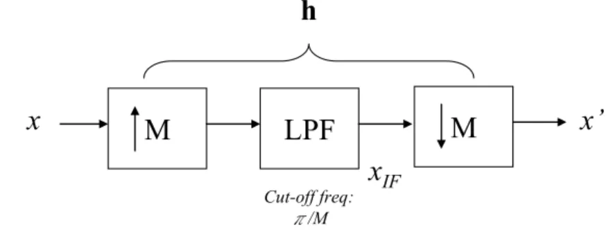
(45) Chapter4. Effects introduced by non-ideal re-sampling blocks. This chapter discusses the phenomenon of the performance difference when we choose different decimation phase p. The motivation to research the characteristics of all the decimation phases is from the derivation of convergence behavior. In practical use, it is enough to choose a “well-behaved” phase among these candidates. But the study of the other phases can provide us thorough information about how the finite length up/down sample filter affects the system performance. Different selection of p may produce different response of hp. Because it is correlated with the update equations listed in chapter 2, when we accidentally choose a phase that suffers from distortion, the performance will consequently degrade. In figure 4.1, if the input x is a WSS (wide-sense stationary) signal, the output x’ should be also a WSS signal after passing through the combined structure of M-fold interpolator and the M-fold decimator (We will prove this in section 4.1). However, some non-ideal effects of the intermediate low pass filter will distort this ideal all pass system.. h. x. M. Cut-off freq: π/M. Figure 4.1. M. LPF. x’. xIF. Combination of equal rate up and down sample blocks.. In this chapter, we will focus on distortion introduced by such non-ideal filter in LMS algorithm. After quantifying such distortion, we will provide a method to avoid the performance degradation.. 37.

(46) 4.1: Properties of random signals through a multi-rate system. Some basic conceptions are introduced when passing a random signal through a multi-rate system. We will show some statistical concepts about x’ in figure 4.1 given a WSS (Wide Sense Stationary) signal x. In this section, all WSS and CWSS processes are assumed to be zero mean.. 4.1.1: Preliminaries. A. L-fold Interpolator Passing an input sequence x(n) into an L-fold interpolator results in. ⎧⎪ x ( n / L ) , if n is an integer multiple of L yI ( n ) = ⎨ , otherwise. ⎪⎩0, whose z transform is. YI ( z ) = X ( z L ) .. (4.1). B. M-fold Decimator Passing an input sequence x(n) into an M-fold decimator results in yD ( n ) = x ( nM ) ,. whose z transform is. YD ( z ) =. 1 M. M −1. ∑ X (z k =0. 1/ M. WMk ) . WM = e − j 2π k / M .. (4.2). C. Cyclo-WSS Process Let R xx ( n, k ) = E ⎡⎣ x ( n ) x* ( n − k ) ⎤⎦ denote the autocorrelation function of x(n). The process is said to be (CWSS)L if. E ⎡⎣ x ( n ) ⎤⎦ = E ⎡⎣ x ( n + kL ) ⎤⎦ , ∀n, k , and 38.

(47) R xx ( n, k ) = R xx ( n + L, k ) , ∀n, k .. D. Linear Periodically Time-Varying (LPTV) system A system is said to be LPTV with period L (denoted as (LPTV)L) if the output. y(n) in response to input x(n) can be written as y (n) =. ∞. ∑ h ( n, k ) x ( n − k ). k =−∞. where the h( n, k ) is an LTI system with property h ( n, k ) = h ( n + L, k ) , ∀n, k .. The LPTV system can be implemented as figure 4.2.. x(n). H0(z) H1(z) y(n) :. :. HL(z) Figure 4.2: Implementation of an (LPTV)L system.. Note: The output at time n is one of the L filters, its order is controlled by number (n mod L).. 39.

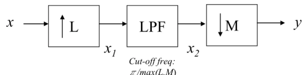
(48) 4.1.2: Properties of the signal passing through a multi-rate system. x. L. M. LPF x1. Cut-off freq: π/max(L,M). y. x2. Figure 4.3: A general multi-rate filter.. For each output node in figure 4.3, we outline three important properties. Property A: If we pass a WSS signal x(n) through an L-fold interpolator, the output x1(n) is CWSS with period L. Property B: If we pass a signal x1(n), (CWSS)L, through an (LPTV)L system, the output x2(n) is CWSS with period L. Property C: If we pass a signal x2(n), (CWSS)L, through an M-fold decimator, the output y(n) is CWSS with period K, where K = L / gcd(L, M). gcd{,} is the greatest common factor operator.. In [3], the above properties have been proved and a theory is developed to make the output y(n) to be WSS in general multi-rate systems. Consider the multi-rate system in figure 4.1 in our case. From properties listed above, it is clear that for an equal up sampling and down sampling rate system, passing a wide-sense stationary signal x to the filter results in a wide-sense stationary signal x’.. 40.

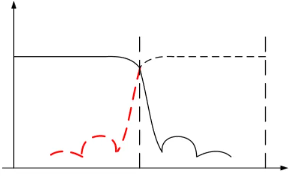
(49) 4.2: Quantification of distortion. In this section, we will first find out the source of distortion. Then the method to evaluate the power of the non-ideal effect is presented. Finally, a frequency domain representation for each node of the reduced complexity structure is derived to provide a theoretical analysis of distortion. This theoretical result will be used to compare with the simulation of the actual distortion signal.. 4.2.1: Source of distortion. Based on the conclusion in section 4.1, the output of the combination of the equal up-sampling and down-sampling rate blocks should be WSS given a WSS input signal. That is, the combined effect should be an all pass filter in frequency domain, and a delta function in time domain. However, some combined effects may produce impulse responses such as appearance of two peaks or asymmetry and distort all-pass property. Because insertion of zeros (interpolation) has nothing to modify, it is easy to assert that the distortion comes from the intermediate low pass filter and the decimation process. Reference to figure 4.1 and set M = 2, we show a brief demonstration of how such non-ideal side lobes of the interpolation filter affects in frequency domain.. Figure 4.4:. Brief demo for non-ideal IF side lobes effect. M = 2. 41.

(50) For M = 2, figure 4.4 shows that the side lobes belonged to the image of 0.5π ~ π affects the frequency components in the neighborhood of 0.5π. Mapping to our system, the filtered output y plays the same role as xIF in this case. That is, we can see the distortion from the filtered output, or the direct identification result, e(n). Distortion of the filtered output means that the adaptive filter operating band is polluted by adjacent image. This implies that the system identification cannot perfectly match the response of the desired signal. Such distortion will reflect on the performance. In section 5.7, we will demonstrate this situation in the spectrum point of view between the distorted filtered signal and the desired signal. Besides, the eigenvalue spread will be shown to point out the performance degradation. It is expected that the adaptive filter suffered from distortion has a larger eigenvalue spread.. 4.2.2: Level of distortion. Next, we present our method to evaluate the distortion power level. Integration shown in (4.3) will be used for our evaluation. Pd = ∫. π /M. a. Φ y (ω ) − Φ d (ω ) d ω .. (4.3). In (4.3), Φy(ω) denotes the power spectrum of the distorted filtered signal in the steady state , and Φd(ω) denotes the power spectrum of the corresponding desired response. Note that the only desired variation in (4.3) is the distortion power, so spectrum samples in our experiment are taken from the Fourier transform of the steady state in time domain where the noisy adaptation has a comparably smaller influence. From the previous section, we know that the distortion occurs in the neighborhood of 42.

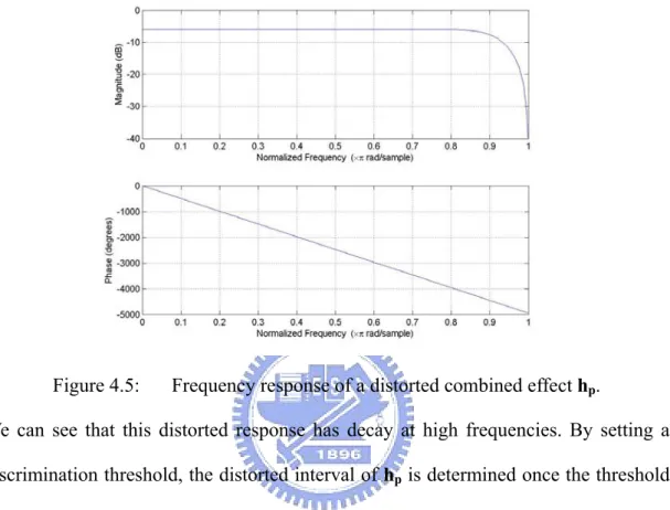
(51) π/M. So the upper bound of the (4.3) is π/M for sure. What we have to do now is to decide the lower bound a. A distorted combined effect of hp is illustrated below.. Figure 4.5:. Frequency response of a distorted combined effect hp.. We can see that this distorted response has decay at high frequencies. By setting a discrimination threshold, the distorted interval of hp is determined once the threshold is exceeded. We first set a default distorted portion for each rate M. The distortion portion defines a default distance between the upper bound and the lower bound of hp, the lower bound must not exceed the default interval to prevent a wrong estimation of the lower bound. Because of the fact that the frequency response is stretched M times wider after the. M-fold decimation, we can determine the distortion interval at the filtered output is 1/M of the estimating distortion interval of hp. Take figure 4.5 as an example. The estimated distortion interval of hp is approximately 0.15π, so the effective distortion interval of the filtered output is approximately 0.15π/M. In (4.3), the lower bound a is now set as 0.85π/M in this case. Notice that if there’s no distortion, a = π/M. 43.

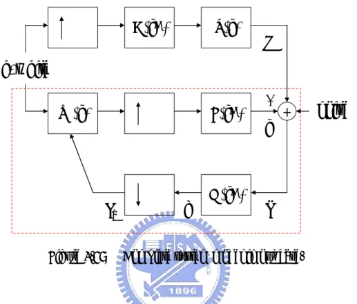
(52) 4.2.3: Frequency domain representation of the reduced complexity structure. M. A(zM). S(z). W(z). M. F(zM). M. G(zM). d. x, white. ep Figure 4.6:. v. -. +. noise. y. e. Complete system model in our case.. For the problem of echo cancellation, S(z) is replaced by the z-transform of the echo path. In figure 4.6, the echo path is modeled at the up-most branch, and the adaptive filter part is the other two branches bracketed with the dashed line. In our system, the echo is sampled at the Nyquist rate. So the echo path is operating in a bandwidth 2M times more narrow than the input signal and we up-sample the input signal to match this requirement. Here, A(zM) is an interpolation filter for channel output. Now we list each node in our system model in z-transform domain. Their transformations will be denoted in capital form. Use (4.1), the z-transform of the desired signal d can be represented as. D ( z ) = A( zM ) S ( z ) X ( zM ). (4.4). and the filtered signal y can be represented as. 44.

(53) Y ( z ) = F ( z M )W ( z M ) X ( z M ) .. (4.5). The z-transform of the error signal e is E ( z) = D( z) −Y ( z) .. (4.6). In section 5.5, we will use equation (4.6) to be our theoretical comparison.. In equation (4.5), we can see that we interpolate the filtered signal to match the desired signal in number. A signal after interpolation has images of the compressed version of the original signal distributed periodically in the high frequency domain. If the interpolation low-pass filter is not ideal, the frequency components beyond the cut-off frequency will not completely filter out. This will influence the performance because these partially suppressed images make the interpolated filtered signal unable perfectly fit the high frequency components of the desired signal. Such high frequency components can be considered as a smaller-level distortion (compared to the distortion in the neighborhood of π/M) in different mismatched rate systems. In section 5.5, spectrums of the filtered signals and the desired signal of different mismatched rates will be demonstrated. We will see that given different mismatched ratio M, different conditions of partially suppressed images will appear in the high frequency domain.. 45.

(54) 4.3: Filter design issue to avoid such degradation. In section 4.2.1, we know that the distortion introduced by the interpolation filter and the different decimation phase is the source, except the noise, that will degrade the performance of the LMS. Because the relatively weak response of hp in the high frequency, the adaptive filter cannot perfectly match the desired response. On the other hand, the distorted hp in the update equation is just like the coloring filter that correlates the input random signal in the conventional LMS. In our knowledge of the adaptive filter theory, such correlation will enlarge the eigenvalue spread and cause the convergence slower. Since the combined response hp is determined once the intermediate low pass filter is set, we can evaluate its frequency response beforehand and choose a flat one to avoid such degradation caused by the imperfection design of filter. Note that the flat frequency response hp can be found not only by changing the intermediate filter, but also by checking all the decimation phases for their corresponding hp. In our simulations, even though there is a certain decimation phase that has larger distortion, there still exist other possible “well behaved” phases that have flat response of hp given the same intermediate filter. These “well behaved” phases will achieve better performance given the same parameters. If we evaluate the frequency responses hp of all the decimation phases, a good choice may be found among them. In section 5.5, given M and the “possibly distorted” filter coefficients, we will demonstrate the coexistence of different performance among each decimation phase. A measurement which represents their corresponding performance difference, called DESR, will also be shown. We shall introduce it in the next section.. 46.

(55) 4.3.1: Distortion to pure Error Signal Ratio (DESR). Finally, we remark a measurement of distortion. To quantify the performance difference between the “well behaved” phase and the distorted phase, we give a performance index, i.e., the Distortion to pure Error Signal Ratio (DESR). It is defined as follows. Suppose phase 1 suffers from distortion. Then the MSE ratio between phase 1 and the MMSE (DESR) is:. DESR ≡. E ⎡⎣e12 ⎤⎦ E ⎡⎣eo2 ⎤⎦. .. (4.7). Because E ⎡⎣eo2 ⎤⎦ provides the optimum solution for solving the system identification problem and the distortion is the only degradation of this performance difference, the distorted E ⎡⎣e12 ⎤⎦ can be written as. E ⎡⎣e12 ⎤⎦ = E ⎡⎣eo2 ⎤⎦ + E ⎡⎣ed2 ⎤⎦ .. (4.8). E ⎡⎣e2d ⎤⎦ represents the distortion power. Now DESR can be written as. DESR =. E ⎡⎣e12 ⎤⎦ E ⎡⎣eo2 ⎤⎦. ≅. E ⎡⎣e d2 ⎤⎦ E ⎡⎣eo2 ⎤⎦. +1 .. (4.9). From (4.13), if the performance is scaled in dB, we can see that the distance between. E ⎡⎣e12 ⎤⎦ and MMSE is the distortion power.. 47.

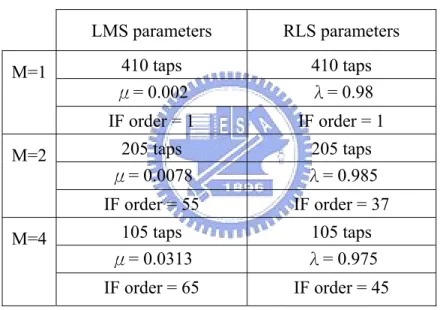
(56) Chapter5. Simulations. In this chapter, promised simulations in the previous sections will be shown. Before entering this chapter, we shall give the environment specifications in our simulation.. Environment settings: Channel: A 400 taps FIR with a low pass shape, cutoff frequency = π/M/2 (Divide by 2 because we sample the channel at the Nyqusit rate). SNR = 150dB. Adaptive filter settings:. M=1. M=2. M=4. LMS parameters. RLS parameters. 410 taps μ= 0.002. 410 taps λ= 0.98. IF order = 1. IF order = 1. 205 taps μ= 0.0078. 205 taps λ= 0.985. IF order = 55. IF order = 37. 105 taps μ= 0.0313. 105 taps λ= 0.975. IF order = 65. IF order = 45. Table 5.1: LMS and RLS filter settings Both rates(M = 2, 4) use Kaiser low pass filter with minimum -133 dB side-lobe attenuation of the Fourier transform of the window.. Note1:. In our simulations, DF coefficients are set equal to the IF coefficients.. Note2:. It is equal to the conventional adaptive algorithm if M = 1.. Note3:. The performance index is the normalized mean square value of the vector. e(n). We will rapidly run ten times to obtain an ensemble average. Note4:. “Covariance windowing” is used for input data sequence if no specification. 48.

(57) 5.1: Original adaptive algorithm V.S. its simplified version. 5.1.1: LMS algorithm. Figure 5.1.1: MSE of original LMS VS simplified version, M = 2.. Figure 5.1.2: MSE of original LMS VS simplified version, M = 4.. We can see that the simplified version converges faster than the original one. As we 49.