Synchronized Reproduction Promotes Species Coexistence through Reproductive Facilitation
Yu-Yun Chen1*, Sze-Bi Hsu2
1
Mathematics Division, National Center for Theoretical Science, Hsinchu, Taiwan, 300
2 Department of Mathematics, National Tsing Hua University, Hsichu, Taiwan,300. *
Corresponding author. Email address: [email protected] (Yu-Yun Chen).
Abstract Theories for species coexistence often describe properties of competitive
relationships between species and predict competitive exclusion when little resource partition exists. Indeed many forest species that compete for resources showed niche differentiation. Yet several forest systems experiencing synchronous reproduction while potentially utilizing the same mutualist pools showed little resource partitioning. Several hypotheses such as pollinator facilitation and predator satiation suggest the synchronized phenomenon as an evolutionary consequence from the cooperative manner in these plants. Theoretical discussion on such systems rarely discussed its means to species coexistence. We propose a two-species model to include
enhancement of reproduction occurs in the event of synchrony. We assume saturations for recruitment and recruitment enhancement for the neighboring species at high participation level, due to resource limitation. Our model demonstrates the influence of adult survival rate, recruitment rate and flowering periodicity on species
persistence. We also observe “rescue” effect from a “superior” species to a “weaker” species even when the later is not self-sustainable. In the past decades, rapid
environmental changes have altered landscape as well as behavior of organisms. Some of the changes are important to the species in the model. Our work may provide some insights to evaluate anthropological impacts on species.
Keywords species coexistence, synchrony, recruitment enhancement, pollination
facilitation, predator satiation, masting, cooperative system, uniformpersistence, monotone maps.
1. Introduction
Species coexistence and mechanisms maintaining species diversity have been the major focuses in ecology. Species sharing the same resources are assumed to
encounter competition from its neighbors and finally result in exclusion of the weaker competitor (Connell et al., 2004; Fargione & Tilman, 2006). Important theories to explain species coexistence in the presence of competition include the niche theory and the theory of storage effect. The niche theory (Harpole & Tilman, 2007; Huchingson, 1959) suggests that competing species can coexist due to niche
differentiation. Yet when individuals of the competing species encounter each other in a close proximity, competitive exclusion occurs. The storage effect (Chesson, 2003; Warner & Chesson, 1985) suggests a significantly reduced competition between species when reproduction is temporally fluctuating and asynchronous between species. The mechanism allows recruitment and establishment of individuals in the inferior competitors by avoiding competition(Chesson, 2003). These hypotheses assume the major interaction of competition between species. However, species inhabiting the same community, even competing for the same resources, sometimes form a cooperative system, e.g. during plant reproduction. The impact of cooperative system on coexistence of species in the same trophic level is rarely discussed.
Plant reproduction is a multi-interaction process: abiotic restrictions determine timing of flowering; biotic interactions determine success of seeding. Abiotic restrictions may appear in several forms. First, resource availability, such as availability of irradiation and soil nutrients, limits reserve levels and reproduction of individuals. Second, climatic cues, such as drought and low ambient temperature, control the development of flower buds and the onset of flowering (Augspurger, 1983; Wood, 1956). Finally, rainfall influences fruit development and subsequent seedling survivorship (Bebber et al., 2002; Williamson & Ickes, 2002).
Major biotic interactions affecting seeding are flower-pollinator relationship and seed-seed predator interaction. The hypothesis of pollinator facilitation suggests a positive relationship between flowering magnitude and the success of pollination (Kelly & Sork, 2002). It remarks that large floral display attracts nomadic pollinators and large quantity of resource (nectar and pollens) enhances recruitment of residential pollinators (Appanah, 1993; Isagi et al., 1997; Sakai, 2002; Satake & Iwasa, 2000). A great attraction for pollinators requires a high-level synchrony among plant
consumed by invertebrate and vertebrate seed predators. (Janzen, 1974) suggested that seeds facing predation may enhance survivorship by two means: extensive length of time with no reproduction and massive production of seeds in a short time
intermittently. Extended intervening intervals between flowering (and fruiting) events cause a decrease in predator populations due to starvation. When the plant population (community) explodes in seeding, the already-low predator populations will then be easily satiated. In consequence, individuals in synchronous reproduction collectively increase the efficiency to satiate predators and facilitate seed survival of the
population (community) as a whole. Cases of massive flower and seed production and predator satiation were evident at both the population and the community level (Curran & Leighton, 2000; Numata et al., 2003; Sakai et al., 1999; van Schaik, 1986). High levels of seed addition to the forest floor enhance seedling recruitment and survival and thus population sustainability (De Steven & Wright, 2002; Wright et al., 2005). Community-level synchrony of seed production increases seed availability (Chen, 2007; Metz et al., 2008; Sun et al., 2007) for species participating in the events thus the community become a cooperative system.
In diverse forests, although experiencing similar climate, species often exhibit variable reproductive patterns (Sakai, 2001). Some species reproduce more frequently while other less frequently. In several occasions species synchronized in flowering and seedling (Appanah, 1985; Corlett, 1990). Although factors triggering
synchronization are yet confirmed (Sakai et al., 2006; Wright & van Schaik, 1994; Yasuda et al., 1999), the phenomenon of synchronous reproduction generates effects predicted by the hypotheses of pollinator facilitation and predator satiation:
recruitment resulted from the synchronized reproductive event is enhanced thus promote sustainability of populations.
To understand the role of the cooperative system through reproduction, we construct models to explore demographical performance in two sympatric species. The two species possess different flowering strategies, by which we mean flowering periodicity in this study. These species are assumed to rely solely on sexual
reproduction for future recruitment and share the same guild of enemies. The species may have the same or different species-specific mortality rates and reproduce in different periods. In the intervening interval between reproductive events, all individuals are assumed to acquire resources in order to recover its reserve level for the next reproductive event. During the time, a population may decrease due to
mortality. If the intervening period is too long, decrease of population during non reproductive season may go beyond tolerable degrees and cause a collapse of the population. We intend to discuss conditions that allow and disapprove coexistence of the two strategies.
2. Models and stability analysis
Two species on focus (populations x and y) reproduce at periodsp1andp2, and have adult survival ratesb1andb2, respectively. The discrete map of populations x and y are the followings:
(
n n)
n f n x y x +1 = , ,(
n n)
n g n x y y +1 = , ,wherexn+1andxnare the abundances of population x at time n+1 and n ;yn+1and
n
y the abundances of population y at time n+1 and n, respectively. Functions f and g describe the interplay of two demographical processes, mortality and recruitment, and the interaction between the two species through facilitation for recruitment. In our models, we ignore two other demographical processes: immigration and emigration.
The sympatric species may reproduce asynchronously when a lag is involved in the reproductive timing of the species. This results in little interaction between the species. When no lag is involved, species may reproduce synchronously at the
common multiples of the species’ periods. We discuss the demographical dynamics of two sympatric species in the above two cases and sections 2.1 and 2.2, respectively.
2.1 Non-synchrony reproduction
We begin our model construction with a simple case when no reproductive synchrony of two species occurs. The discrete map for the dynamics of either species is written as = + = ≠ = + + ) (mod 0 ) ( ) (mod 0 1 1 p n x h bx x p n bx x n n n n n (1) , providedx0 >0and0< b<1.
At the individual level, flower and fruit production is restricted by resource availability thus an upper bound of reproduction is present. Furthermore, when a plant population is sufficiently large, the increase of per capita seed production rate may
slow down due to saturation of pollinators. We thus assume that the recruitment functionh(xn) follows a Michaelis-Menten kinetics, in which a maximum
recruitment rate ( u ) for the species occurs when the population is sufficiently large. The function is written as
n n n x k ux x h + = ) (
where the half-saturation constant k >0. From (1), we obtain the p-map
) ( p 1 n n p p n b x h b x x+ = + −
For convenience, we rewrite the above model as ) ( ) (x b x h b 1x f x= = p + p−
We take the derivative off(x), f'(x)=bp+bp−1h'(bp−1x), where 0 ) ( ) ( ' 2 > + = x k uk x h .
A fixed pointx=0always exists and is asymptotically stable whenσ <1, where k u b b f'(0) p p 1 := = + −
σ . When
σ
>1, the fixed pointx=0is unstable and there exists a unique fixed pointx*>0(Appendix, Theorem 1). We reformulateσ <1 andobtain p bp
k u b −1 <1−
, where1−bpis the cumulative mortality rate and
k u bp−1 is the recruitment rate at the time p when the population is small. This is, when recruitment rate is smaller than mortality rate, population decreases and goes extinct from the community. Whenσ >1, we have p bp
k u
b −1 >1− . Sustainability of population x is assured under the condition that recruitment rate at the time p is greater than cumulative mortality rate. The population size is predicted to be
1 1 ) 1 ( ) 1 ( * − − − − − = p p p p b b b k ub x when
σ
>1.We further explore species-specific demographical properties that influence sustainability of a species. The ratio of maximum recruitment rate andthe
half-saturation constant, u/k, indicates the marginal effect of the population on recruitment. When population size is finite, a high u/k means a larger per capita increment in recruitment rate compared to a low u/k. The value of the ratio u/k may be
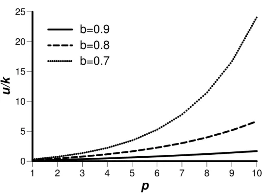
determined by the investment produce a seed. For example, food resource provided to pollinators, advertisement effect that helps to recruit pollinators, size of seed sets, and protection for seeds, etc. A population that reproduces infrequently (a large p) requires a larger marginal increase of recruitment rate to sustain the population. For a
population with low adult survival rate ( b ), this requirement of per capita enhancement on recruitment rate is stricter even under a relatively frequent reproduction (Figure 1).
2.2 Synchronous reproduction
In this case, the two species reproduce at periods ofp1andp2, respectively.
Synchronized reproduction of two species takes place at a period of the least common multiples ( p ) ofp1andp2, where p=m1p1=m2p2andm1andm2are positive integers. Parametersm1andm2are the frequencies of flowering during the interval ofn=1to
p
n= for species x and y, respectively.
When two species reproduce simultaneously, the community exhibits a large floral display and presents a large quantity of resources for pollinators thus enhances pollination rates. Massive flowering is then followed by mast fruiting that enhances seed survivorship. Both processes contribute to enhancement of reproduction in both species. The effect of reproductive facilitation follows the Michaelis-Menten kinetics due to resource limitation and saturation of pollinators. The recruitment enhancement functions are written as
n n y a y v l + + = 1 1 1 1 and n n x a x v l + + = 2 2
2 1 , wherev1andv2are
maximum enhancement rates for species x and y, respectively. Parametersa1anda2are the half-saturation sizes of the populations.
The models are as the following:
(
)
( )
( )
( )
( )
( ) ( )
= = + ≠ = + ≠ = ) (mod 0 ), (mod 0 ) (mod 0 ), (mod 0 ) (mod 0 , , 2 1 1 1 2 1 1 1 p n p n y l x h x F p n p n x h x F p n x F y x n f n n n n n n n n (2)(
)
( )
( )
( )
( )
( ) ( )
= = + ≠ = + ≠ = ) (mod 0 ), (mod 0 ) (mod 0 ), (mod 0 ) (mod 0 , , 2 1 2 2 1 2 2 2 p n p n x l y h y G p n p n y h y G p n y G y x n g n n n n n n n n (3)n n n x k x u x h + = 1 1 1( ) and n n n y k y u y h + = 2 2
2( ) , whereu1andu2are maximum recruitment rates for species x and y, respectively, when reproduce alone.
We rewrite (2) and (3) into the following p-maps after routine computations:
+ = = + = = − − − − − − − − − − )) ( ( )) ( ( ) ( ) , ( )) ( ( )) ( ( ) ( ) , ( ) 1 ( 1 1 2 ) 1 ( 1 2 2 ) 1 ( 2 ) 1 ( 1 2 1 ) 1 ( 1 1 1 ) 1 ( 1 1 1 2 2 2 2 2 2 1 1 1 1 x f b l y g b h y g b y x G y y g b l x f b h x f b y x F x m p m p m p m p m p m p (A2) where ) ( ) ( 1 1 1 1 1 1 x b h x b x f = p + p− 4 4 4 3 4 4 4 2 1 L times m m x f f f f x f 1 ) 1 ( 1 1 ( ) ( ( ( ( )))) − − = . ) ( ) (y b2 2y h2 b2 2 1y g = p + p − 4 4 3 4 4 2 1 L times m m x g g g y g 1 ) 1 ( 2 2 ( ) ( ( ( ))) − − =
In appendix (Lemma 2) we show that every positive orbit (+ , ) =
{
( , )}
∞=00
0 y n n n
x x y
O ,
providedx0,y0>0, is bounded.
To analyze stability of fixed points, we first obtain the Jacobian of the discrete map (A2) at(x,y): ∂ ∂ ∂ ∂ ∂ ∂ ∂ ∂ = y G x G y F x F y x J( , ) (4) where )) ( )))( ( ( )) ( ( ' ( )) ( ))( ( ( ' )) ( ( )) ( ))( ( ( ' )) ( ( )) ( )))( ( ( )) ( ( ' ( ) 1 ( ) 1 ( 1 1 2 ) 1 ( 1 2 2 1 2 2 ) 1 ( ) 1 ( 1 1 2 1 1 ) 1 ( 1 2 2 ) 1 ( ) 1 ( 1 2 1 1 2 ) 1 ( 1 1 1 ) 1 ( ) 1 ( 1 2 1 ) 1 ( 1 1 1 1 1 1 2 1 1 2 2 2 2 1 1 1 1 2 2 2 2 2 2 1 1 1 2 2 1 1 1 1 y g dy d x f b l y g b h b b y G x f dx d x f b l b y g b h x G y g dy d y g b l b x f b h y F x f dx d y g b l x f b h b b x F m m p m p p p m m p p m p m m p p m p m m p m p p p − − − − − − − − − − − − − − − − − − − − − − − − + = ∂ ∂ = ∂ ∂ = ∂ ∂ + = ∂ ∂ (5)
The fixed point(0,0)
SinceF(0,0)=0andG(0,0)=0, (0,0)is a fixed point of the map (A2). From (5) we have
1 1 1 1 1 1 1 1 1 1 1 1 1 1 1 1 1 1 ) ( )) 0 ( ' )( ( ) 0 , 0 ( λ = + = + = ∂ ∂ − − − m p p m p p k u b b f k u b b x F 0 ) 0 , 0 ( = ∂ ∂ y F 0 ) 0 , 0 ( = ∂ ∂ x G 2 2 2 1 2 2 1 2 2 1 2 2 2 2 2 2 2 2 ) ( )) 0 ( ' )( ( ) 0 , 0 ( λ = + = + = ∂ ∂ − − − m p p m p p k u b b g k u b b y G Let ( ) 1 1 1 1 1 1 1 1 k u b bp + p− = σ and ( ) 2 2 1 2 2 2 2 2 k u b b p + p − =
σ . Thenλ1andλ2are eigenvalues ofJ(0,0). The fixed point(0,0)is locally asymptotically stable ifσ1 <1andσ2 <1. We restateσ1 <1andσ2 <1as 1 1 1 1 1 1 1 1 p p b k u b − < − (6) 2 2 2 2 2 1 2 1 p p b k u b − < − (7)
Terms on the left hand side of (6) and (7) are recruitment rates of the two populations while the terms on the right hand side are the mortality rates. Theorem 3 (Appendix) provides sufficient conditions for the conclusion that when both mortality rates exceed the recruitment rates, both populations reach extinction at the steady state. The
demographical dynamics of population x is independent from that of population y in this case. That is, when both populations are unable to sustain themselves (Figure 2, region A), recruitment facilitation does not prevent the extinction of the species. When recruitment rates are higher than mortality rates, i.e.σ1 >1andσ2 >1, both populations are sustainable and could reach a steady state with population sizes of
c
x andyc(Theorem 7, appendix; Figure 2, region D).
The first eigenvalueλ is enlarged by 1 m1 power and the second eigenvalueλ by 2
m2 power compared to the eigenvalue in the one-dimension case. The parameters m1
and m2 are positive integers indicating frequencies of reproduction during the time
1 =
fixed point(0,0)but the speed of convergence of trajectories towards the equilibrium point. When m1 and m2 are large, the system converges fast to the fixed point(0,0).
The fixed point(x*,0)
Whenσ1>1, there exists a unique fixed point(x*,0). For the evaluation of fixed point(x*,0), we observe the behavior of model (A2) under the condition thaty=0. The model becomes one-dimensional (A1) around the fixed point(x*,0).
0 , )) ( ( ) ( 1 ( 1) ) 1 ( + > =b f − x h b − f − x x x p m p m (A1)
Whenσ >1 and 1 σ <1, the fixed point2 (x*,0)exists and we have
1 1 1 1 1 1 1 1 * 1 1 1 1 ) 1 ( ) 1 ( − − − − − = p p p p b b b k b x µ >0
From Theorem 4 (Appendix), x*is the unique positive root of f(x)= x.
To evaluate stability of the fixed point(x*,0), we obtain the Jacobian ofthe map
(A2) at(x*,0): ∂ ∂ ∂ ∂ ∂ ∂ ∂ ∂ = ) 0 *, ( ) 0 *, ( ) 0 *, ( ) 0 *, ( ) 0 *, ( x y G x x G x y F x x F x J .
From (5) and Theorem 4 (i) (Appendix) the eigenvalues ofJ(x*,0)are
(
'( *))
1 ) 0 *, ( 1 1 = < ∂ ∂ = x f x m x F λ and x m p p p p p k u b b x b l k u b b x y G σ λ + = + = ∂ ∂ = − − − − : ) ( *) ( ) 0 *, ( 1 2 2 1 2 2 1 1 2 2 2 1 2 2 2 2 2 2 1 2 2 . (8)The parameterσ describes dynamical behavior of population y, which is a function of x the net population growth ratesσ , 1 σ and the reproduction enhancement rate (2 v2).
When the population y sustains itself without reproductive facilitation, i.e.σ2>1, σ x is always greater than 1 and the fixed point(x*,0)is unstable (Remark 1, appendix). Thus population y is maintained despite the behavior of population x. Under the condition ofσ1>1and0<σ2 <1(a community with only species x when no
inter-specific interaction is considered), small recruitment enhancement (a small v2)
in the system (Region B1, figure 1). On the other hand, a sufficiently large
enhancement (a large v2) leads toσ >1 and the fixed pointx (x*,0)becomes unstable.
The recruitment enhancement by species x enables y to maintain its population (σ >1, x Region B2, figure 2). In this case, the two species coexist in the system.
Requirement of recruitment enhancement varies between communities, i.e. the difference inσ and1 σ . We reformulate2 σ =1 to explore conditions needed to maintain x
population y under a givenσ <1. 2
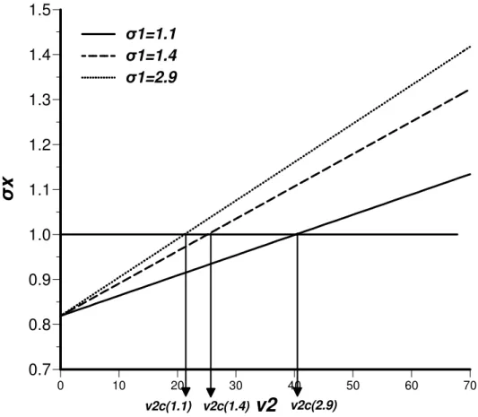
Let − + − − + = = c m− p− p c x v k b a k k u b v H 2 1 1 1 2 1 1 2 2 1 2 2 1 2 2 ) 1 ( ) 1 ( ) 1 ( ) ( 1 2 2 σ σ σ σ σ (9)
We show that strength of recruitment enhancement (v2) negatively correlated with the
net population growth rateσ (Figure 3). 1
The fixed point(0,y*)
We apply the one dimensional analysis (Appendix) to examine the stability
of(0,y*)and obtain the parameterσ the second eigenvalue of the Jacobiany J(0,y*):
1 1 1 1 1 1 1 2 1 1 1 1 1 1 1 1 1 2 1 1 ) *))( ( ( + − − + − − = p p p p p m y k u b b y b l k u b b σ
Using similar underlying principles described in the previous section, we distinguished region C1 and C2 of figure 1 with the following rules:
Letσ2 >1and0<σ1<1.
(i) Ifσy <1, then(0,y*)is asymptotically stable. (ii) Ifσy >1, then(0,y*)is unstable.
Thus we conclude that a sufficiently strong reproductive facilitation for population x from population y allows invasion of species x to the system even though x is not self-sustainable. Similar to the case of(x*,0), the strength of recruitment enhancement (ν ) strongly influences whether species x could invade the system. 1
Species coexistence
Coexistence of two species is possible when both species are self-sustainable (σ1>1 andσ2 >1). However, it is also possible to have species coexistence even when one of the species has a net population growth (σ ) smaller than 1. We reformulate σ >1 x
and σ >1 as the followings: y 2 2 1 2 2 2 1 2 1 1 2 2 2 1 2 1 2 ( *) 1 p m p p m b x b l k u b > − ⋅ ⋅ − − − − σ σ (10) 1 1 2 1 1 1 1 1 1 2 1 1 1 1 1 1 1 ( *) 1 p m p p m b y b l k u b > − ⋅ ⋅ − − − − σ σ (11)
where parametersm1andm2are frequencies of flowering for species x and y during the
time length of p, respectively. Opposite to the case of fixed point(0,0)(Region A, figure 2), parametersm1andm2not only affects the speed of convergence but also the
invasion of species y to the system of species x (Region B2, figure 2) or vice versa (Region C2, figure 2). In region B2, described by (10), a largem2(i.e. a smallp2),
which implies a higher frequency of reproduction (up to the time p) for species y, lowered the requirement for v2 so that (10) holds. The same principle applies for the
invasion by species y.
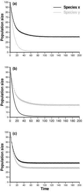
We conjecture that the uniqueness of the positive fixed point holds for the parameter regions B2, C2, and D ,We run the simulation under the set of condition for the case of B2 (σ1 >1, σ2 <1, and σx >1): b1= b2 =0.9, p1=1, p2 =2,
2 / 1 1 k =
u , u2/k2 =0.1, v1/a1 =2, v2/a2 =4.3, x0 =100, andy0 =100. Figure 4(a) provides periodic solutions for both species x and y (x∞ >0andy∞ >0). We show simulations for C2 and D in figure 4(b) and 4(c), respectively. For both cases,
0
> ∞
x andy∞ >0and there exists a unique positive fixed point which is
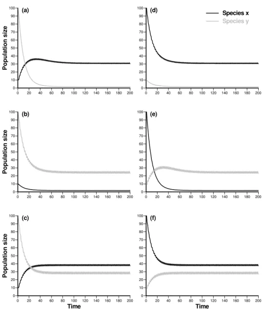
asymptotically stable. Our simulations show that the outcomes for parameter regions B2, C2, and D are independent from the initial conditions(x0,y0)(Figure 5).
3. Discussion
Organisms of the same trophic level are often assumed to compete for resources thus may only coexist when competition is reduced to minimum, both spatially and temporally (Chesson et al., 2004). Yet cooperative systems are evident in nature, not only for species in different trophic levels (e.g. plants and pollinators) but also for species potentially compete for the same set of resources. We model such a system and observe conditions where reproductive facilitation is in aid for species
coexistence and where the effect of facilitation does not affect the demographic outcome.
We show that when no between-species interaction is considered,
species-specific recruitment and mortality rates determines whether a species can persist in the community. No discussion is made on how the demographical dynamics of the two species may interact under the circumstance. Most often, interest in species coexistence may lead to the consideration of interactions such competition for such a case even in the absence of cooperative effect. Previous studies of competition concluded competitive exclusion for a community. Yet when recruitment is low, perhaps due to inefficient pollination and high seed predation, significance of competition is reduced.
Our model in the synchronous case demonstrates the general form describing periodic reproduction and the recruitment enhancement effect of synchronous
reproduction between two species. A special case of this form is whenp2is a multiple
ofp1, i.e.m2=1in the model of section 2.2. This special case is important because most cases in natural systems belong to this type: the most common flowering periods are periods of 0.5, 1, and 2 (Sakai 2002). In the case of synchrony, relations of the two population fall into three major types: (1) neither species can persist (Region A of figure 2), (2) only the one species persists (Regions B1 and C1 of figure 2), and (3) two species coexist (Regions B2, C2, and D of figure 2). The first case of extinction of both species occurs when neither of the net population growth rates is greater than one. In forest communities, recruitment rates for species are usually low. Thus adult survival and reproductive periodicity is relatively important for populations. When periods of reproduction is extremely long or when adult survival rates are low, net growth rate may be reduced and lead to extinction. This is particularly evident in disturbed area and often lead to loss of species. In the second outcome of only one species persists, the species has a net population growth greater than one will not need reproductive facilitation from the other species to help maintain its population. In the third case, two sources can be identified for species coexistence. (I) When both species exhibit population growth rates greater than one, coexistence is evident. (II) Coexistence is possible via strong reproductive facilitation. A “weaker” species with a σ <1 could be “rescued” by the “superior” species, which has aσ >1, before the population of the “weaker” species is driven to extinction due to mortality. We suspect that in some cases rare species might benefit from masting events due this rescuing effect. However, empirical data is needed to support this observation.
The models in the present study assume a cooperative system with two species and discuss how “cooperative” behavior may help to maintain species coexistence. In recent years, anthropological activities have changed global and local landscape (Appanah & Manaf, 1994; Bernard, 2004; Burgess, 1971; Curran et al., 1999). Some parameters in our model are influenced by these rapid changes. For example,
flowering behavior as well as pollinator availability may change under global warming. In addition, logging and landscape alternation for human use change adult survival rates significantly. Change of forest environments for the above reasons also alters recruitment rates for species. Parameterization of the model may help to evaluate the impact of rapid environmental changes on such a system thus species coexistence. However, our model does not provide the scope to explore all cases with more between-species interactions, which are likely changed during the alteration of landscape. Neither do we consider variable strength of interactions between young and mature generations. To realize our model, an improvement to a multi-stage model with the populations of adult trees and seedlings is necessary. The model shall also consider different competitive and cooperative strengths for the generations. We intend to investigate these effects in the future.
Acknowledgement
We thank the Mathematics Division of National Center for Theoretical Sciences, National Science Concil, Republic of China for providing postdoctoral fellowship to Yu-Yun Chen during the study. The reseach is partially supported by National Science Council, Republic of China. We are also in debt for all the logistic support by the National Tsing Hua University.
0
5
10
15
20
25
u
/k
1
2
3
4
5
6
7
8
9
10
p
b=0.9
b=0.8
b=0.7
Figure 1 Correlation between reproductive period and index of marginal increase of recruitment rate (u/k) when σ =1. We show three cases with adult survival rate b=0.7, 0.8, and 0.9, respectively.
Figure 2 Phase diagram. This case contains two reproductive periods p1 and p2.
The condition of σ <1 and1 σ <1 leads to extinction of both species (Region A). The 2
condition of σ >1 and1 σ >1 leads to the coexistence of two species (Region D). 2 Under the condition that σ >1 and1 σ <1, species x becomes the sole existence for the 2 system if σ <1 (Region B1). When x σ >1 and1 σ <1, species y could invade the 2
system if σ >1 (Region B2). Under the condition that x σ >1 and2 σ <1, species y 1 becomes the only survivor when σ <1. Species x could only invade the system when y
y
0.7
0.8
0.9
1.0
1.1
1.2
1.3
1.4
1.5
σ
x
0 10 20 30 40 50 60 70v2
σ
1=1.1
σ
1=1.4
σ
1=2.9
v2c(1.1) v2c(1.4) v2c(2.9)Figure 3 Correlation between parameters σ and x v2. The three inclining lines and
the line of σ =1 intersect at x v2c, the lower bound of v2c needed so that population y
0 10 20 30 40 50 60 70 80 90 100 P o p u la ti o n s iz e 0 10 20 30 40 50 60 70 80 90 100 P o p u la ti o n s iz e 0 10 20 30 40 50 60 70 80 90 100 P o p u la ti o n s iz e 0 20 40 60 80 100 120 140 160 180 200 0 20 40 60 80 100 120 140 160 180 200 0 20 40 60 80 100 120 140 160 180 200 Time Species x Species y (a) (b) (c)
Figure 4 Time series for populations x and y under conditions of (a)B2:, u1/k1=2, u2/k2=0.1, v1/a1=2, v2/a2=4.3; (b) C2: u1/k1=2, u2/k2=0.1, v1/a1=2, v2/a2=4.3; (c) D: u1/k1=2, u2/k2=0.1, v1/a1=2, v2/a2=4.3. Species x and y have the same adult survival
rates b1=b2=0.9 and their reproductive periods are p1=1, p2=2. Initial conditions for all
0 10 20 30 40 50 60 70 80 90 100 P o p u la ti o n s iz e 0 10 20 30 40 50 60 70 80 90 100 P o p u la ti o n s iz e 0 10 20 30 40 50 60 70 80 90 100 P o p u la ti o n s iz e 0 10 20 30 40 50 60 70 80 90 100 0 10 20 30 40 50 60 70 80 90 100 0 10 20 30 40 50 60 70 80 90 100 0 20 40 60 80 100 120 140 160 180 200 0 20 40 60 80 100 120 140 160 180 200 0 20 40 60 80 100 120 140 160 180 200 Time 0 20 40 60 80 100 120 140 160 180 200 0 20 40 60 80 100 120 140 160 180 200 0 20 40 60 80 100 120 140 160 180 200 Time Species x Species y (a) (b) (c) (d) (e) (f)
Figure 5 Time series for populations x and y under conditions of (a) B2, (b) C2, and (c) D. All conditions follows figure 4 except the initial conditions: simulations (a)-(c) start from x0=10, and y0=100 and simulations (d)-(f) x0=100, and y0=10. All
three cases showed species coexistence and (x∞, y∞) are the same despite the
Appendix: Mathematical analysis of the asymptotic behavior of the maps (A1), (A2). One-dimensional dynamics
Consider the following one-dimensional map
0 , )) ( ( ) ( : ) ( = ( 1) + 1 ( 1) > =F x b f − x h b − f − x x x p m p m (A1)
where m is a positive integer,
0 , , 1 0 , ) ( , ) ( ) ( 1 < < > + = + = − b u k x k ux x h x b h x b x f p p 4 4 3 4 4 2 1o oLo times k k x f f f x f − = ( ) ) ( ) ( Theorem 1: Let{ }∞1, 0 >0 = x
xn n be the iterates generated by the map (A1) and
k u b bp p 1 := + − σ . Then
(i) If σ <1, thenlim =0 ∞ → n
n x .
(ii) If σ >1, thenlimxn x*
n→∞ = wherex* is the unique positive fixed point of the
map (A1). Moreover, x*satisfies 1 1 ) 1 ( ) 1 ( * − − − − − = p p p p b b b k ub x , x*= f(x*),0< f'(x*)<1.
Proof: It is easy to verify the following: 0 ) ( ) ( ' 2 > + = x k uk x h , 0 ) ( 2 ) ( '' 3 < + − = x k uk x h , '( )= p + '( p−1 ) p−1 >0 b x b h b x f , , 0 ) )( ( '' ) ( '' x =h bp−1x bp−1 2 < f 0 )) ( '' ) ( ( ' )) ( ( ' ) ( ' )) ( ( ' )) ( ))( ( ( '' )) ( ( 0 ) ( ' )) ( ( ' )) ( ( ' )) ( ( ) 1 . 1 ( ) 3 ( ) 2 ( ) 3 ( ) 2 ( ) 2 ( ) 1 ( 2 2 ) 3 ( ) 2 ( ) 1 ( < + + = > = − − − − − − − − − x f x f f x f f x f x f f x f dx d x f f x f dx d x f x f f x f f x f dx d A m m m m m m m m m L L L L 0 ) 0 ( ) 0 ( , ) 0 ( ' = + −1 ( ) = = f f k u b b f p p k , . ) ( )) 0 ( ' ( ) ) 0 ( ' ( )) ( ( ) 0 ( ' 1 ) 1 ( 1 0 ) 1 ( m p p m p p x m b k u b f b h b x f dx d F σ = + = + ⋅ = − − − = −
Suppose there are two positive fixed points xˆ1, xˆ2 with 0<xˆ1 <xˆ2. ThenF(0)=0, )
ˆ ( ˆ1 F x1
x = andxˆ2 =F(xˆ2). By Rolle’s Theorem, there existsˆx , 3 ˆx , 4 2
4 1
3 ˆ ˆ ˆ
ˆ
0< x <x <x <x such thatF'(xˆ3)=1andF'(xˆ4)=1. Apply Rolle’s Theorem again, there exists ˆx , 5 xˆ3 <xˆ5 < xˆ4such thatF ''(xˆ5)=0. However, from (A1.1) for
anyx>0, '( )=( + '( −1 ( −1)( )) −1)( f( −1)(x))>0 dx d b x f b h b x F p p m p m , 0 )) ( ( ) )) ( ( ' ( )) ( ))( ( ( '' ) ( '' ) 1 ( 2 2 1 ) 1 ( 1 2 ) 1 ( 1 ) 1 ( 1 < + + = − − − − − − − − x f dx d b x f b h b x f dx d b x f b h x F m p m p p m p m p
This leads to a contradiction.
Ifσ <1thenF'(0)<1. From the uniqueness of positive fixed point, the monotonicity ofF(x)andF(x)< xfor x large, it follows that the curvey=F(x)is below the liney =x. Thuslim =0
∞ → n
n x . Ifσ >1thenF'(0)>1. Then there exists a unique positive
fixed point *x . The monotonicity ofF(x)implies thatlimxn x*
n→∞ = . We note thatx*= F(x*)= f(f(m−1)(x*))= f(m)(x*). From the uniqueness of positive fixed point, we havex*= f(x*). It is easy to verify that
* ) 1 ( *) ( ' 1 1 1 1 1 1 1 1 1 x b k b k b x f p p p − + − + = <1. Two-dimensional dynamics
Consider the following two-dimensional p-map
)) ( ( )) ( ( ) ( ) , ( )) ( ( )) ( ( ) ( ) , ( ) 1 ( 1 1 2 ) 1 ( 1 2 2 ) 1 ( 2 ) 1 ( 1 2 1 ) 1 ( 1 1 1 ) 1 ( 1 1 1 2 2 2 2 2 2 1 1 1 1 x f b l y g b h y g b y x G y y g b l x f b h x f b y x F x m p m p m p m p m p m p − − − − − − − − − − + = = + = = (A2) where0<b1,b2 <1, m1, m2, p1, andp2are postivie integers,m1p1 =m2p2 = p,
. 2 , 1 , 0 , , 1 ) ( , 1 ) ( , 2 , 1 , 0 , , ) ( , ) ( ), ( ) ( ), ( ) ( 2 2 2 1 1 1 2 2 2 1 1 1 1 2 2 2 1 1 1 1 2 2 1 1 = > + + = + + = = > + = + = + = + = − − i a v X a X v X l Y a Y v Y l i k u Y k Y u Y h X k X u X h y b h y b x g x b h x b x f i i i i p p p p (A2.1)
Lemma 2: Every positive orbit (+ , ) =
{
( , )}
∞=00
0 y n n n
x x y
O of the map (A2) withx0,y0 >0 is bounded.
Proof: From the map (A2) and (A2.1), we have )) ( ( ) 1 ( ) ( : ) ( ~ ) , ( )) ( ( ) 1 ( ) ( : ) ( ~ ) , ( ) 1 ( 1 2 2 2 ) 1 ( 2 ) 1 1 ( 1 1 1 1 ) 1 ( 1 2 2 2 2 1 1 1 y g b h v y g b y G y x G x f b h v x f b x F y x F m p m p m p m p − − − − − − + + = ≤ + + = ≤ (A2.2) Let
{ }
x~n , ~x0 = x0,{ }
yn , y~0 = y0 be the iterates generated by the maps) ( ~ ), ( ~ y G y x F
x= = , respectively. Claim: xn ≤ ~xn, yn ≤ ~yn, n=1,2L. From the monotonicity of F~(x) and (A2.2), we have
. ~ ) ~ ( ~ ) ( ~ ) , ( , ~ ) ~ ( ~ ) ( ~ ) , ( , ~ ) ( ~ ) , ( 1 1 1 1 2 1 1 1 1 2 1 0 0 0 1 n n n n n n F x y F x F x x x x x F x F y x F x x x F y x F x = ≤ ≤ = = ≤ ≤ = = ≤ = − − − − M
Similarly we can prove that yn ≤ ~yn, forn=1,2,L,n. By Theorem 1, either 0 ~ lim = ∞ → n n x or 0 ~ ~ lim = * > ∞ → n n n x x . Hence
{ }
∞ =0 n nx is bounded. Similarly, we have that
{ }
∞=0
n n
y is bounded. Thus we complete the proof of Lemma 2.
Theorem 3: Let 2 2 1 2 2 2 1 1 1 1 1 1 2 2 1 1 : , : k u b b k u b b p + p− = p + p− = σ σ .
(i) If σ1 <1,σ2 <1, then the fixed point(0,0)is asymptotically stable.
(ii) If ~ (1 ) 1 1 1 1 1 1 1 1 1 1 + + < = − k v u b bp p σ , then lim =0 ∞ → n n x . (iii) If ~ (1 ) 1 2 2 2 1 2 2 2 2 2 < + + = − k v u b b p p σ , then lim =0 ∞ → n n y . Proof:
(i) The local stability of(0,0)is established in Section 2.2.
(ii) From the proof of Lemma 2 and Theorem 1, we have xn ≤~xn and 0 ~ lim = ∞ → n n x . Hence 1 ~ 1< σ implies lim =0 ∞ → n n x .
(iii) Similarly, σ~2 <1 implies lim =0 ∞ → n
n y .
+ + = + + = − − − − − − − − *) ( : *) ( : 1 2 1 1 1 1 1 1 1 1 1 1 1 1 1 1 2 2 2 1 2 2 1 2 2 1 2 2 2 1 1 1 1 1 1 2 2 2 2 2 y b l k u b b k u b b x b l k u b b k u b b p p p m p p y p p p m p p x σ σ (A2.3) Theorem 4: Let 0<σ2 <1,σ1 >1.
(i) If σx <1, then the fixed point(x*,0)of the map (A2) is asymptotically stable, where *x is the unique fixed point of x=b1p1f(m1−1)(x)+h1(b1p1−1f(m1−1)(x)). (ii) If σx <1 and 2 2 2 1 2 2 2 ) 1 ( ~ 2 2 k v u b b p + p + = − σ <1, then(x*,0)is globally asymptotically stable.
(iii) Ifσx >1, then there exists a positive fixed point(xc,yc)of the map (A2) satisfyingxc > x*.
Proof: (i) From (5) and (8) we have ( *,0)=0 ∂
∂
x x G
. Hence from Theorem 1 (ii) and (5) the eigenvalues of J(x*,0) are
(
'( *))
(
'( *))
(
'( *) 1)
) 0 *, ( 1 1 11 11 1 1 1 1 1 1 1 = + = < ∂ ∂ = p p− p− m− m x f x f x b h b b x x Fλ
(
)
(
)
(
)
x m p m p p p g x b l g x b l h b b x y G σ λ ( *,0) 2 2 '(0) ( 1 *) '(0) 2 ( 11 *) '(0) 2 : 1 2 1 1 1 2 2 1 2 2 2 = + ⋅ ⋅ = = ∂ ∂ = − − − −Thus if σx<1 then(x*,0)is asymptotically stable.
(i) The local stability of(x*,0)is established in the Section 2.2. (ii) From Theorem 3 (iii), it follows that lim =0
∞ → n
n y . Then the asymptotic stability of
) 0 *,
(x implies that lim(xn,yn) (x*,0)
n→∞ = .
(iii) For any fixed y≥0, from Theorem 1 and the hypothesisσ1 >1, there exists a unique positive fixed pointϕ( y)ofx=F(x,y). Obviouslyϕ(0)= x*andϕ( y)is strictly increasing in y. Consider the mapy=G(ϕ(y),y). It is easy to verify
that x y y y G dy d σ ϕ = =0 ) ), (
( . Thus the conditionσx >1 implies the existence of a
unique positive fixed pointycof the mapy=G(ϕ(y),y).
Remark 1: Sinceσ~2 <1 impliesσx <1, it is impossible that 1 ~
2 <
σ in case (iii) of Theorem 4.
Similarly, we have the following Theorem. Theorem 5: Let0<σ1<1,σ2 >1, then
(i) ifσy <1, then the fixed point(0,y*)of the map (A2) is asymptotically stable where *y is the unique positive fixed point of
)) ( ( ) ( 2 2 1 ( 1) ) 1 ( 2 2 2 2 2 y g b h y g b y= p m − + p − m− . (ii) Ifσy <1and 1 1 1 1 1 1 1 ) 1 ( : ~ 1 1 k v u b bp + p + = −
σ <1, then(0,y*)is globally asymptotically stable.
(iii) If σy >1, then there exists a positive fixed point(xc,yc)of the map (A2)
satisfyingyc > y*.
Remark 2: Sinceσ~1 <1 impliesσy <1, it is impossible thatσ~1 <1 in case (iii) of Theorem 5.
Theorem 6: Ifσ1>1 andσ2 >1, then there exists a positive fixed point(xc,yc)of the map (A2) withxc > x*andyc > y*.
Proof: From (A2.3) we note thatσ1>1 impliesσy >1 andσ2 >1 impliesσx >1.
For any fixedx≥0, from Theorem 1 the mapy=G(x,y) has a unique positive fixed pointϕ(x). Obviouslyϕ(0)= y*andϕ(x)is strictly increasing in x. Consider the mapx= F(x,ϕ(x)). It is easy to verify that ( , ( )) 1
0 > = = y x x x F dx d σ ϕ . Hence by
Theorem 1, there exists a unique positive fixed pointxcofF(x,ϕ(x))satisfyingxc > x*. Thus there exists a positive fixed point(xc,yc)withyc =ϕ(xc)> y*.
In the following we shall state the results about the global behavior of the iterates of the map (A2), provided that the uniqueness of the positive fixed point(xc,yc)holds. Definition: Consider a discrete mapx= f(x)where
{
x x x i n}
R C f f f R R f n n i n n n , ( ) , ( ), 0, 1,2, , : 1 1 1L ∈ = L ≥ = L = → + + + . We say thediscrete systemx= f(x)is cooperative if ( )≥0 ∂ ∂ x x f j
i for alli≠ and for allj n
R x∈ +. Theorem A (Jiang, 1994, Theorem C): Let p be a fixed point of the cooperative
systemx= f(x). Assume that for each n
R
x∈ +, the positive orbitO+(x) is bounded. If p is a unique fixed point then p is globally asymptotically stable inR+n.
Remark 3: In his paper, Jiang prove Theorem A for a cooperative systemx'= f(x). It is easy to verify that the Theorem A also holds for a cooperative mapx= f(x). For the mathematical properties of cooperative map the reader may consult the review paper by Hirsch and Smith (2005).
LetX Rn, X0 Int(Rn), X0 bdry(Rn) + +
+ = ∂ =
∈ .
Definition: A discrete mapx= f(x), f :X →X is said to be uniformly persistent with respect toX0, X∂ 0 if there existsη >0such that ∂ ≥η
∞
→ ( ( ), )
limInfd fn x X0
n for
allx∈X0.
The following is a uniform persistence Theorem for discrete mapx= f(x). Theorem B (Freedman and So, 1987): Let the following (1)-(7) hold. (1) f :X →X is a continuous function.
(2) f(∂X0)⊂∂X0
(3) f(X0)⊆ X0
(4) O+(x)is a bounded positive orbit for allx∈X
(5) f ∂X0is dissipative
(6) f ∂X0has an acyclic coveringπ =
{
M1LMR}
(7) There is no positive orbit
{ }
+
∈Z
n n
x such that
{ }
xn n∈Z ⊂W+(Mi)+ for some i . Then
the mapx= f(x) is uniformly persistent with respect to∂X0.
Applying Theorem A and Theorem B to the map (A2) yields the following results: Theorem 7: Let
(i) σ1 >1 andσ2 >1,
(ii) σ1 >1,0<σ2 <1, andσx >1, (iii) σ2 >1,0<σ1<1, andσy >1.
If one the (i)-(iii) holds then the map (A2) is uniformly persistent. Furthermore if the positive fixed point(xc,yc)is unique then(xc,yc)is globally asymptotically stable in
2 +
R
Proof: We only prove the theorem for case (i). The case (ii) and (iii) can be proved using similar arguments. Let σx >1 and σy >1. Then(x*,0)and(0,y*)are repellers
with respect toInt(R+2). Thus by Theorem B, the map (A2) is uniformly persistent. From Theorem A, if the positive fixed point(xc,yc)is unique then(xc,yc)is globally asymptotically stable in ( 2)
+
R
Int .
Remark 4: We conjecture that under either of the assumptions (i), (ii), (iii), the positive fixed point(xc,yc)of the map (A2) is unique.
References
Appanah, S., 1985. General flowering in the climax forests of Southeast Asia. J. Trop. Ecol. 1, 225-240.
Appanah, S., 1993. Mass flowering of dipterocarp forests in the aseasonal tropics. J.Bioscience 18, 457-474.
Appanah, S., Manaf, M.R.A., 1994. Fruiting and seedling survival of dipterocarps in a logged forest. J. Trop. For. Sci. 6, 215-222.
Augspurger, C.K., 1983. Phenology, Flowering Synchrony, and Fruit-Set of 6 Neotropical Shrubs. Biotropica 15, 257-267.
Bebber, D., Brown, N., Speight, M., 2002. Drought and root herbivory in understorey Parashorea Kurz (Dipterocarpaceae) seedlings in Borneo. J. Trop. Ecol. 18, 795-804.
Bernard, H., 2004. Effects of selective logging on the microhabitat-use patterns of non-volant small mammals in a Bornean tropical lowland mixed-dipterocarp forest. Nat. Human Act. 8, 1-11.
Burgess, P.F., 1971 The Effect of Logging on Hill Dipterocarp Forest. Malayan Nat. J. 24, 231-237.
Chen, Y.-Y., 2007. Reproductive phenology in a lowland dipterocarp forest and its consequences for seedling recruitment. Ph. D Dissertation, University of Georgia, Athens, Georgia.
Chesson, P., 2003. Quantifying and testing coexistence mechanisms arising from recruitment fluctuations. Theor. Popul. Biol. 64, 345-357.
Chesson, P., Gebauer, R.L.E., Schwinning, S., Huntly, N., Wiegand, K., Ernest, M.S.K., Sher, A., Novoplansky, A., Weltzin, J.F., 2004. Resource pulses, species interactions, and diversity maintenance in arid and semi-arid environments. Oecologia 141, 236-253.
Connell, J.H., Hughes, T.E., Wallace, C.C., Tanner, J.E., Harms, K.E., Kerr, A.M., 2004. A long-term study of competition and diversity of corals. Ecol. Monogr. 74, 179-210.
Corlett, R.T., 1990. Flora and Reproductive Phenology of the Rain Forest at Bukit Timah Singapore. J. Trop. Ecol. 6, 55-63.
Curran, L.M., Caniago, I., Paoli, G.D., Astianti, D., Kusneti, M., Leighton, M., Nirarita, C.E., Haeruman, H., 1999. Impact of El Nino and logging on canopy tree recruitment in Borneo. Science 286, 2184-2188.
Curran, L.M., Leighton, M., 2000. Vertebrate responses to spatiotemporal variation in seed production of mast-fruiting Dipterocarpaceae. Ecol. Monogr. 70,
101-128.
De Steven, D., Wright, S.J., 2002. Consequences of variable reproduction for seedling recruitment in three neotropical tree species. Ecology 83, 2315-2327.
Fargione, J., Tilman, D., 2006. Plant species traits and capacity for resource reduction predict yield and abundance under competition in nitrogen-limited grassland. Funct. Ecol. 20, 533-540.
Freedman, H.I., So, J., 1989. Persistence in discrete semidynamical system. SIAM J. Math. Anal. 20, 930-938.
Harpole, W.S., Tilman, D., 2007. Grassland species loss resulting from reduced niche dimension. Nature 446, 791-793.
Hirsch, M.W., Smith, H., 2005. Monotone map: a review. J. Differ. Equ. Appl. 11, 379-398.
Huchingson, G.E., 1959. Homage to Santa Rosalia or why are there so many kinds of animals. Am. Nat. 93, 145-159.
Isagi, Y., Sugimura, K., Sumida, A., Ito, H., 1997. How does masting happen and synchronize? J. Theor. Biol. 187, 231-239.
Janzen, D.H., 1974. Tropical blackwater rivers, animals, and mast fruiting by the Dipterocarpaceae. Biotropica 4, 69-103.
Jiang, J.F., 1994. On the global stability of cooperative systems. Bull. London Math. Soc., 26, 455-458.
Kelly, D., Sork, V.L., 2002. Mast seeding in perennial plants: Why, how, where? Annu. Rev. Ecol. Syst. 33, 427-447.
Metz, M.R., Comita, L.S., Chen, Y.Y., Norden, N., Condit, R., Hubbell, S.P., Sun, I.F., Noor, N., Wright, S.J., 2008. Temporal and spatial variability in seedling dynamics: a cross-site comparison in four lowland tropical forests. J. Trop. Ecol. 24, 9-18.
Numata, S., Yasuda, M., Okuda, T., Kachi, N., Noor, N.S.M., 2003. Temporal and spatial patterns of mass flowerings on the Malay Peninsula. Am. J. Bot. 90, 1025-1031.
Sakai, S., 2001. Phenological diversity in tropical forests. Popul. Ecol. 43, 77-86. Sakai, S., 2002. General flowering in lowland mixed dipterocarp forests of South-east
Sakai, S., Harrison, R.D., Momose, K., Kuraji, K., Nagamasu, H., Yasunari, T., Chong, L., Nakashizuka, T., 2006. Irregular droughts trigger mass flowering in
aseasonal tropical forests in Asia. Am. J. Bot. 93, 1134-1139.
Sakai, S., Momose, K., Yumoto, T., Nagamitsu, T., Nagamasu, H., Hamid, A.A., Nakashizuka, T., 1999. Plant reproductive phenology over four years including an episode of general flowering in a lowland dipterocarp forest, Sarawak, Malaysia. Am. J. Bot. 86, 1414-1436.
Satake, A., Iwasa, Y., 2000. Pollen coupling of forest trees: Forming synchronized and periodic reproduction out of chaos. J. Theor. Biol. 203, 63-84.
Sun, I.-F., Chen, Y.-Y., Hubbell, S.P., Wright, S.J., Noor, N.S.M., 2007. Seed predation during general flowering events of varying magnitude in a Malaysian rain forest. J. Ecol. 95, 818-827.
van Schaik, C.P., 1986. Phenological changes in a Sumatran rain forest. J. Trop. Ecol. 2, 327-347.
Warner, R.R., Chesson, P.L., 1985. Coexistence Mediated by Recruitment
Fluctuations - a Field Guide to the Storage Effect. Am. Nat. 125, 769-787. Williamson, G.B., Ickes, K., 2002. Mast fruiting and ENSO cycles - does the cue
betray a cause? Oikos 97, 459-461.
Wood, G.H., 1956. The dipterocarp flowering season in North Borneo, 1955. Malayan Forester. 19, 193-201.
Wright, S.J., Muller-Landau, H.C., Calderon, O., Hernandez, A., 2005. Annual and spatial variation in seedfall and seedling recruitment in a neotropical forest. Ecology 86, 848-860.
Wright, S.J., van Schaik, C.P., 1994. Light and the phenology of tropical trees. Am. Nat. 143, 192-199.
Yasuda, M., Matsumoto, J., Osada, N., Ichikawa, S.e., Kachi, N., Tani, M., Okuda, T., Furukawa, A., Rahim, N.A., Manokaran, N., 1999. The mechanism of general flowering in Dipterocarpaceae in the Malay Peninsula. J. Trop. Ecol. 15, 437-449.