Copyright © 2013 Inderscience Enterprises Ltd.
ZigBee-based long-thin wireless sensor networks:
address assignment and routing schemes
Meng-Shiuan Pan*
Department of Computer Science and Information Engineering, Tamkang University, 215 Taipei, Taiwan E-mail: [email protected] *Corresponding author
Yu-Chee Tseng
Department of Computer Science, National Chiao Tung University, 300 Hsin-Chu, Taiwan
E-mail: [email protected]
Abstract: Although Wireless Sensor Networks (WSNs) have been extensively researched, its deployment is still a big concern. This paper makes two contributions to this issue. First, we promote a new concept of Long-Thin (LT) topology for WSNs, where a network may have a number of linear paths of nodes as backbones connecting to each other. These backbones are to extend the network to the intended coverage areas. At the first glance, a LT WSN only seems to be a special case of numerous WSN topologies. However, we observe, from real deployment experiences, that such a topology is quite general in many applications and deployments. The second contribution is that we show that the address assignment and thus the tree routing scheme defined in the original ZigBee specification may work poorly, if not fail, in a LT topology. We then propose simple, yet efficient, address assignment and routing schemes for a LT WSN. Simulation results are reported. Keywords: address assignment; pervasive computing; routing; wireless sensor network; ZigBee. Reference to this paper should be made as follows: Pan, M-S. and Tseng, Y-C. (2013) ‘ZigBee-based long-thin wireless sensor networks: address assignment and routing schemes’, Int. J. Ad Hoc and Ubiquitous Computing, Vol. 12, No. 3, pp.147–156.
Biographical notes: Meng-Shiuan Pan received the PhD. degree in Computer Science from
National Chiao Tung University. He is an Assistant Professor of Department of Computer Science and Information Engineering, Tamkang University. His research interests include Wireless Sensor Network, Mobile Computing and LTE-A networks.
Yu-Chee Tseng got his PhD in Computer and Information Science from the Ohio State University in January of 1994. He was Chairman (2005–2009), Chair Professor (2011–present) and Dean (2011-present), Department of Computer Science, National Chiao-Tung University, Taiwan. He received Outstanding Research Award (National Science Council, 2001, 2003 and 2009), Best Paper Award (Intl Conf. on Parallel Processing, 2003), Elite I. T. Award (2004) and Distinguished Alumnus Award (Ohio State University, 2005) and Y.Z. Hsu Scientific Paper Award (2009). His research interests include Mobile Computing, Wireless Communication and Parallel and Distributed Computing. An IEEE Fellow, He served on the Editorial Boards of IEEE Trans. on Vehicular Technology (2005–2009), IEEE Trans. on Mobile Computing (2006–2011) and IEEE Trans. on Parallel and Distributed Systems (2008–present).
1 Introduction
The rapid progress of wireless communication and embedded micro-sensing MEMS technologies has made Wireless Sensor Networks (WSN) possible. A WSN usually needs to
configure itself automatically and support ad hoc routing. A lot of research works have been dedicated to WSNs, including power management (Ye et al., 2002), routing and transportation (Braginsky and Estrin, 2002; Eghbali et al.,
sensors are divided into clusters and clusters are logically divided into layers. A cluster is a small group and sensors in a cluster contend to different node addresses. The real address of a sensor will be the concatenation of node address, cluster address and layer address. The basic concept of (Ould-Ahmed-Vall et al., 2005) is similar to the ZigBe address assignment. Before assigning address, the sink constructs a tree to calculate the subtree size of each intermediate node. Each intermediate node locally reserves enough address spaces for its descendants and carefully assign addresses to its children. In (Schurgers et al., 2002), the authors propose a distributed address assignment scheme, which aims to reduce message overhead when solving address conflict. After choosing an unused address, a node first encodes its address and then broadcasts it. Nodes use the received code word to detect if there are address conflicts. The above three works (Ali and Uzmi, 2004; Ould-Ahmed-Vall et al., 2005; Schurgers et al., 2002) are designed for general WSNs and cannot be used in LT or ZigBee networks. There are two works (Pan et al., 2009) and (Yen and Tsai, 2010) discuss the network formation protocols for ZigBee networks. The proposed schemes in (Pan et al., 2009) and (Yen and Tsai, 2010) are aimed to improve the address utilisation in ZigBee networks but cannot be directly applied in LT WSNs. Reference (Li et al., 2008) and (Qiu et al., 2009) design enhancements for ZigBee routing protocols. In (Li et al., 2008), the authors propose to modify ZigBee AODV routing scheme to utilise ZigBee tree information. A relay node finds the destination is located in its subtree can switch to use ZigBee tree routing to relay packets. But most routing paths in LT WSNs are along linear paths, the AODV routing scheme is not suitable. Reference (Qiu et al., 2009) presents a similar idea to (Li et al., 2008). In this work, we adopt the idea of ZigBee tree routing to design our routing protocol and nodes can find some shortcuts on the linear paths to quickly relay packets.
This paper extends the preliminary work (Pan et al., 2008) in the following ways: 1) introducing a systematic network planning flows for network managers; 2) proposing a node ranking procedure to guarantee the address assignment result as be as planned; 3) modifying address assignment scheme to utilise node ranking results; 4) discussing link maintenance; 5) expanding the performance evaluations.
The rest of this paper is organised as follows. Preliminaries are given in Section 2. Section 3 presents our algorithms. Performance evaluations are given in Section 4. Finally, Section 5 concludes this paper.
2 Preliminaries
2.1 ZigBee address assignment
In ZigBee, network addresses are assigned to devices by a distributed address assignment scheme. Before forming a network, the coordinator determines the maximum number of children of a router (Cm), the maximum number of child routers of a router (Rm) and the depth of the network (Lm). Note that children of a router can be routers or end devices, so Cm > Rm. The coordinator and routers can each have at most 2011), sensor deployment and coverage issues (Huang et al.,
2004; Sung and Yang, 2010) and localisation (Ahmed et al., 2005). In the application side, health care is discussed in (Huo et al., 2011) and navigation is studied in (Tseng et al., 2006).
In this paper, we discuss the Long-Thin (LT) network topology, which seems to have a very specific architecture, but may be commonly seen in many WSN deployments in many applications, such as gas leakage detection of fuel pipes, carbon dioxide concentration monitoring in tunnels,stage measurements in sewers, street lights monitoring in highway systems, flood protection of rivers and vibration detection of bridges. In such a network, nodes may form several long backbones and these backbones are to extend the network to the intended coverage areas. A backbone is a linear path which may contain hundreds of sensor nodes and may go beyond thousands of meters. So the network area can be scaled up easily with limited hardware cost.
Recently, several WSN platforms have been developed. For interoperability among different systems, standards such as ZigBee (ZigBee, 2006) have been developed. In the ZigBee protocol stack, physical and MAC layer protocols are adopted from the IEEE 802.15.4 standard (IEEE 802.15.4, 2003). ZigBee solves interoperability issues from the physical layer to the application layer. ZigBee supports three kinds of network topologies, namely star, tree and mesh networks. A ZigBee coordinator is responsible for initialising, maintaining and controlling the network. A star network has a coordinator with devices directly connecting to the coordinator. For tree and mesh networks, devices can communicate with each other in a multihop fashion. The network is formed by one ZigBee coordinator and multiple ZigBee routers. A device can join a network as an end device by associating with the coordinator or a router. In ZigBee, a device is said to join a network successfully if it can obtain a 16-bit network address from the coordinator or a router. ZigBee specifies a distributed address assignment scheme, which allows a parent device to locally compute addresses for child devices. While the assignment scheme has low complexity, it also prohibits the network from scaling up and thus cannot be used in LT networks.
In this paper, we propose address assignment and routing schemes for ZigBee-based LT WSNs. To assign addresses to nodes, we design rules to divide nodes into clusters. Each node belongs to one cluster and each cluster has a unique cluster ID. All nodes in a cluster have the same cluster ID, but different node IDs. The structure of a ZigBee network address is divided into two parts: one is cluster ID and the other is node ID. Following the same ZigBee design philosophy, the proposed scheme is simple and has low complexity. Moreover, similar to the ZigBee tree routing protocol, the proposed routing protocol can also utilise nodes’ network addresses to facilitate routing. In addition, routing can take advantage of shortcuts for better efficiency, so our scheme does not restrict nodes to relay packets only to their parent or child nodes as ZigBee does.
Existing works (Ali and Uzmi, 2004; Ould-Ahmed-Vall et al., 2005; Schurgers et al., 2002) have discussed address assignment for WSNs. Ali and Uzmi (Ali and Uzmi, 2004) propose a hierarchical address assignment scheme, where
if it is the destination or one of its child end devices is the destination. If so, this router will accept the packet or forward this packet to the designated child end device. Otherwise, it will relay packet along the tree. Assume that the depth of this router is d and its address is A. This packet is for one of its descendant devices if the destination address Adest satisfies
A<Adest <A + Cskip(d – 1) and this packet will be relayed to the child router with address
dest ( 1) 1 ( ). skip( ) r A A A A Cskip d C d − + = + ×
If the destination is not a descendant of this device, this packet will be forwarded to its parent. In ZigBee tree routing, each node can only choose its parent or child as the next node. Since no shortcut can be taken, this strategy may cause longer delay in LT networks.
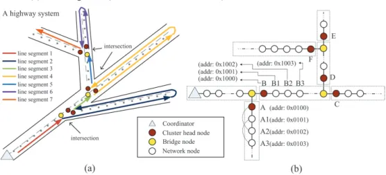
3 LT WSN: Formation, addressing and routing Our goal is to automatically form a LT WSN, give addresses to nodes and conduct routing. Figure. 2(a) shows an example of a LT WSN. For simplicity, we assume that all nodes are router-capable devices. To form the network, nodes are divided into multiple clusters, each as a line segment. For each cluster, we define two special nodes, named cluster head and bridge. The cluster head (resp., the bridge) is the first (resp., last) in the line segment. As a special case, the coordinator, is also considered as a cluster head. The other nodes are network nodes (refer to Fig. 2(b)). A cluster C is a child cluster of a cluster C’ if the cluster head of C is connected to the bridge of C’. Reversely, C’ is the parent cluster of C. Note that a cluster must have a linear path as its subgraph. But it may have other extra links beside the linear path. For example, in Figure 2(b), there are two extra radio links (A, A2) and (A1, A3)in A’s cluster. To be compliant with ZigBee, we divide the ZigBee 16-bit network address into two parts, an m-bit cluster ID and a (16 – m)-bit node ID. The value of m will be discussed later on. The network address of a node v is thus expressed as (Cv,Nv), whereCv and Nv are v’s cluster ID and node ID, respectively. 3.1 Node placement
Before deploying a network, the network manager needs to carefully plan the network by the following three steps. First, the network manager has to mutually identifies clusters according to maps or charts of the target area by the following two principles.
1 The network manager traverses linear paths of the target area from the coordinator in a depth-first manner. 2 When there is a intersection, the network manager
identifies the traversed path as a cluster and consider the following paths as new clusters.
Figure 2(a) shows an example, where there are three intersections and the network can be divided into seven line segments (clusters). Second, after identifying clusters, the Rm child routers and at least Cm – Rm child end devices.
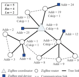
Devices’ addresses are assigned in a top-down manner. For the coordinator, the whole address space is logically partitioned into Rm + 1 blocks. The first Rm blocks are to be assigned to the coordinator’s child routers and the last block is reserved for the coordinator’s own child end devices. From Cm, Rm and Lm, each router computes a parameter called Cskip to derive the starting addresses of its children’s address pools. The Cskip for the coordinator or a router in depth d is defined as: 1 1 ( 1), if 1. skip( ) 1 ,otherwise. 1 Lm d Cm Lm d Rm C d Cm Rm CmRm Rm − − + × − − = = + − − − (1)
The coordinator is said to be at depth d = 0 and d is increased by one after each level. Address assignment begins from the ZigBee coordinator by assigning address 0 to itself. If a parent node at depth d has an address A parent, the n-th child router is assigned to address Aparent + (n – 1) × Cskip(d) + 1 and n-th child
end device is assigned to address Aparent + Rm × Cskip(d) + n. An
example of the address assignment is shown in Figure 1. The Cskip of the coordinator is obtained from Equation (1) by setting d = 0, Cm = 5, Rm = 4 and Lm = 2. Then the child routers of the coordinator will be assigned to addresses 0 + (1 – 1) × 6 + 1 = 1, 0 + (2 – 1) × 6 + 1 = 7, 0 + (3 – 1) × 6 + 1 = 13, etc. The address of the only child end device of the coordinator is 0 + 4 × 6 + 1 = 25. Note that the length of a network address is 16 bits; thus, the maximum address capacity is 216 = 65536. Obviously, the above
assignment is much suitable for regular networks, but not for LT WSNs (where the monitored area may contain hundreds of sensor nodes in a linear path). For example, when setting Cm = 4 and Rm = 2, the depth of the network can only be 14. Also, when there are some LT backbones, the address space will not be well utilised.
Figure 1 A ZigBee address assignment example (see online version for colours)
2.2 ZigBee tree routing protocol
In a ZigBee network, the coordinator and routers can directly transmit packets along the tree without using any route discovery. When a router receives a packet, it first checks
After deploying network nodes, the network can be initialised automatically by each node periodically broadcasting HELLO packets including its IEEE 64-bit MAC address, 16-bit network address (initially set to NULL) and role. In this work, we consider only symmetric links. A communication link (u, v) is established only if u receives v’s HELLO including u as its neighbour and the HELLO’s signal quality is above a threshold. Note that the signal quality should be the average of several packets. Then each node can maintain a neighbour table containing its neighbours’ addresses, roles and ranks. After such HELLO exchanges, the coordinator will start a node ranking algorithm to differentiate nodes’ distances to it (Section 3.2). Then, a distributed address assignment procedure will be conducted to assign network addresses to nodes (Section 3.3).
3.2 Node ranking
We extend the concept of one-dimensional ranking algorithm in (Lotker et al., 2004) to assign a rank to each node. Nodes’ rank values reflect their distances following the line segments to the coordinator. For example, in Figure 2(b), we can see that the distance from Al to the coordinator is shorter than the one from A2 to the coordinator. After the ranking procedure, the rank result will be A1 < A2. In this work, nodes decides their ranks in a distributed manner and all nodes except the coordinator will perform the same procedure. Initially, the rank of the coordinator is 0 and all other nodes have a rank of K, where K is a positive constant. At the end of the algorithm, each node will have a stable rank. The rank value facilitates our address assignments which will be described in Section 3.3.
Except the coordinator, all other nodes will continuously change their ranks. The coordinator will periodically broadcast a Heartbeat packet with its rank. On receiving a Heartbeat, a node will rebroadcast it by including its current rank. After receiving all its neighbours’ Heartbeat packets, a node will calculate its new rank by averaging its neighbours’ ranks. Since the coordinator’s rank is fixed, after receiving several Heartbeat packets, nodes that locate closer to the coordinator will have lower ranks.
Now we give the details of the ranking algorithm. The format of Heartbeat is Heartbeat (sender’s 64-bit address, network manager needs to carefully plan the placement of
cluster heads, bridges and network nodes by the following rules: 1 For each cluster, the first and the last nodes are pre-assigned (manually) as cluster head and bridge, respectively.
2 A cluster head that is not the coordinator should have a link to the bridge of its parent cluster.
3 Conversely, the bridge of a cluster which has child clusters should have a link to the cluster head of each child cluster.
4 Place sufficient network nodes in each cluster to ensure the network connectivity.
Third, after planning the placement of nodes, the network manager can construct a logical network GL to decide some
network parameters. In GL, each cluster is converted into a single node and the parent-child relationships of clusters are converted into edges. For example, Figure 3 is the logical network of Figure 2(b). From GL, we can determine the
maximum number of children CCm of a node in G L and
the depth CLm of GL.By CCm and CLm, we can know that
this network will have at least CN = −1 CCmCLm+1/1−CCm clusters.Then the network manager can decide the value of m (which determines how many clusters in this network) such that 2m-1 <CN £ 2m is satisfied. Nodes are mutually placed based on the above network plan.
Figure 3 The logical network of Fig. 2(b) (see online version for colours)
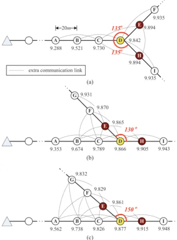
Figure 4 shows some results, where the inter-node distance is 20 m and the transmission range is 45 m. The ranking result in Figure 4(a) is in-order. In Figure 4(b), the ideal ranking result should satisfy B<C<D<E<F. Unfortunately, the result satisfies B<C<E<D<F.
Figure 4 Some ranking examples (see online version for colours)
The ranks of some members of E’s cluster are smaller than the ones of some members of H’s cluster because some E’s members are affected by some members of its parent cluster. We see that D and E have the same number of neighbours but D’s rank is affected by some H’s cluster members. This makes D’s rank higher than E’s, causing the final ranking result not in-order. In Figure 4(c), F and G have smaller ranks than E because they are affected by A’s and B’s ranks. To summarise, we observe that if some members of a cluster have links to the cluster’s parent cluster members, the ranking result may not be in-order.
Here we make two remarks. First, compare to ZigBee network formation protocol, the ranking procedure requires nodes to broadcast extra Heartbeat packets. Let n be the total number of Heartbeat packets from the coordinator. The additional message complexity as opposed to ZigBee for each node is O(n). Second, if a ranking result is in-order, it will facilitate our address assignment and thus network formation. Even if a ranking result is not in-order, we can still assign addresses. After assigning address, a node can refine its address if it overhears a neighbour’s beacons having seq, rank). In the beginning, the coordinator broadcasts a
Heartbeat (coordinator, 0, 0). Then it periodically broadcasts Heartbeat packets, each time with an incremented seq, until seq >h, where h is the maximum hop count distance from the coordinator to any node, which can be easily obtained when planning the network. The operations taken by a non-coordinator node v are defined as follows.
1 On receiving a Heartbeat(u, u’s seq, u’s rank), v checks if it has broadcast a Heartbeat with this sequence number seq. If not, v updates its sequence number to this received seq and broadcasts a Heartbeat (v, v s seq, v’s rank). Then v keeps a record of the pair (u’s seq, u’s rank). If v has received all its neighbours Heartbeat packets with the same seq as its own, it updates its rank to the average of its neighbours ranks (not including its own rank). Otherwise, it sets a timer WaitHeartbeat.
2 When timer WaitHeartbeat times out, v broadcasts a NACK(L), where L is the list of neighbours whose Heartbeats are still missing. Then it sets another WaitHeartbeat timer, until the maximum number of retries is reached.
3 When v receives a NACK(L) such that v ∈ L,it broadcasts a Heartbeat (v, v s seq, v’s rank).
The above step 1 enforces a node to broadcast its rank whenever a new seq is received. New seqs are issued by the coordinator. A node can update its rank after receiving ranks of all its neighbours with the same seq as its own. Steps 2 and 3 are to guarantee reliability due to the fact the broadcast is unreliable in wireless networks. Note that when the coordinator broadcasts the first Heartbeat, only those one hop neighbours of the coordinator can change their ranks. When the coordinator broadcasts the next Heartbeat, those one hop and two hop neighbours can modify their ranks. So, in this scheme, the coordinator needs to broadcast at least h + l Heartbeat packets to guarantee that every node can modify its initial rank. During the ranking procedure, the coordinator’s zero rank value gradually diffuses to the rest of the nodes and thus decreases their ranks. At the end of the algorithm, each node can record its neighbours’ final ranks in its neighbour table. We say that a ranking result is in-order if for each cluster,
• the cluster head (resp., bridge) has the smallest (resp., largest) rank value,
• the ranks of cluster members correspond to their distances to the cluster head and
• the bridge node s rank value is smaller than the ranks of the cluster s child cluster members.
In a linear path topology, the above ranking method can effectively achieve in-order ranking since the coordinator keeps its rank value as zero and continuously pull down the ranks for nodes that locate close to it. As a result, the nodes rank values increment from the coordinator to the last node of the linear path. However, a LT WSN may have some branches and thus the ranking result may not always be in-order.
beacons. There is a special design in this algorithm to refine the address assignment when the ranking result is not in-order. After getting an address, a node u may reconnect to a new parent by the following procedure. Assume a node u, which is not a cluster or a bridge, receives a beacon from a neighbour node u’. Node u checks if u’ is located in the same cluster as it. If not, u will track if u’ beacon for a period of time to see if the signal quality of u’ is better than its current parent v. If u identifies u’ is better than v, u sends Disassociation Request to its children and to v and then re-associates to u’. We will give an example to show the effectiveness of the above reconnect procedure later. Since the address assignment works in a distributed manner, this algorithm eventually stops when all nodes obtain their network addresses.
We say that an address assignment result is as planned if • each pair of cluster head and bridge are assigned to the
same cluster ID and
• each bridge is correctly connected to its child cluster heads.
Below, we make two observations about the address assignment results. First, if the ranking result is in-order and the nodes near-by each cluster head can receive stronger signal from its own cluster head than from others, the address assignment will be as planned. For example, in Figure 4(a), the network will be formed as planned. Second, there are some cases that the formed network is as planned even if the ranking result is not in-order. For example, in Figure 4(b), assuming B as the beacon sender, B will accept nodes C and D with D as the bridge. Although F may send an Association Hequest to B, B will not accept F according to step 1.b of the algorithm. More specifically, when B examines its list, B stops assigning address when the bridge D is encountered. There is another example in Figure. 4(c). Assuming A as the beacon sender, A may accept B, C, F and G. After the cluster head E connects to bridge D, E can start to broadcasts its beacons. Note that at this time F and G is located in the parent cluster of E. When F and G receive E’s beacon, they know that E’s cluster ID is not as theirs. Then F realises that E is a better choice than its original parent A. so do G may reconnect to E or F. After F and G choose their new parents, the address assignment can be as planned.
3.4 Routing rules
Routing in our LT WSN can be purely based on the above address assignment results. Through HELLO packets, a node can collect its neighbours network addresses. Suppose that a node v at logical depth d receives a packet with a destination address (Cdest,Ndest).If v is the destination, it simply accepts this
packet. Otherwise, v performs the following procedures. • If the destination is a neighbour of v, v sends this packet
to the destination directly.
• If Cdest = Cv, the destination is within the same cluster.
Node v can find an ancestor or a descendant in its neighbour table, say, u such that Cu = Cdest and the value
better signal quality than those from its parent. Details will be elaborated further later on.
3.3 Distributed address assignment
The basic idea of our address assignment is as follows. The assignment of cluster IDs depends on the maximum number of branches in the logical network GL. If CCm = l, then the network is a linear path and the address assignment is a trivial job. If CCm > 2, then we follow the style of ZigBee to assign addresses in a recursive and distributed manner. The coordinator has an ID of 0. For each node at depth d in GL, if its cluster ID is C, then its i-th child cluster is assigned a cluster ID of C +(i – l) × CCskip(d) + l, where
1 ( ) . 1 CLm d CCm CCskip d CCm − − = −
Figure 3 shows the assignment result for the network in Figure 2(b). Since each cluster is a linear path, node IDs of the cluster members can be assigned sequentially. Starting from the cluster head with an address of 0, the rest of the nodes can gradually increment their node IDs following the former ranking results, until the bridge node is reached. In Figure 2(b), we have shown some assignment results, where each address is expressed in Hex and the first two symbols represent the cluster ID and the last two represent the node ID.
Now we present the detail algorithm. It is started by the coordinator by broadcasting beacons with the predefined CCm and CLm. When a node u ‘without’ a network address receives a beacon, it will send an Association .Request to the beacon sender. If it receives multiple beacons, the node with the strongest signal strength will be selected. When the beacon sender, say, v at a logical depth d, receives the association request(s), it will do the following:
• If v is not a bridge node, it sets a parameter N = Nv + l (note that when entering this procedure, v already obtains its address (Cv , Nv)). Then it sorts these request senders
according to their ranks in an ascending order into a list L. Then v sequentially examines each node v’ ∈ L. There are two cases:
• If v’ is a cluster head node, v skips v’ and continues to examine the next node in L.
• Otherwise, v assigns address (Cv , N)tov’ and increments N by l . Then v replies an Association Response to v’ with this address. In case that v’ is a bridge node, v stops examining L; otherwise v loops back and continues to examine the next node in L.
• If v is a bridge node, it only accepts requests from cluster heads. At most CCm requests will be accepted and v will reply to the i-th least ranked cluster head, i < CCm, an Association Response with an address (Cv + (i –
l) × CCskip(d) + l, 0). Note that, these cluster heads need to set their logical depths to d +l.
When the node u obtains an address, it will use the MLME-START primitive defined in IEEE 802.15.4 to start its
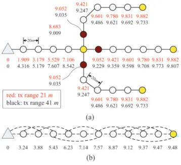
Figure 5 Some ranking results (see online version for colours)
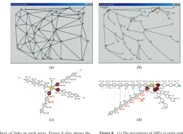
Based on the above model, we generate networks in a 4.8 km × 3.2 km field with adjacent nodes evenly separating by a distance of 20 m. We set the maximum transmission ranges of nodes to be 8l m, i.e., the receiver can detect the sender s signal if the distance between sender and receiver is not longer than 8l m. The signal strength detected by a receiver degrades according to the square of distance between sender and receiver. As mentioned in Section 3.2, the ranking result may not be in-ordered. For example, in Figure 6(b) the nodes marked in black small circles are not in-ordered ranked. Figure 6(c) shows the network topology for region A (the dotted lines are the order of address assignment). We can see that the descendant of B1 is not as planned since B2
connects to B1’s parent cluster. After B1 gets its address and
broadcasts its beacon, B2 will reconnect to B1. Again, Figure
6(d) shows the ranking result and the network topology of region B. In this case, nodes B2, B3 , , B6, which are planned to
be the descendants of B1, are connected by B1’s parent cluster
members. B1 cannot find a neighbour to form its cluster,
resulting in the descendants of B6 being disconnected from
the network. B6 can join this network after its ancestors B2–B5
in the linear path joining to the cluster formed by B1. Here, we
call these temporarily disconnected nodes as orphans. Figure 7 shows that before nodes reconnecting procedure, nodes can still be assigned to the desired address with high probability (>94%)even when there are not-in-order ranked nodes. In average, less than 3% of the nodes will become orphans in our simulations. This result indicates that the network formation can connect all nodes with high probability before some nodes having to reconnect to new parents. Figure 8 shows the percentages of 100% in-order ranking and no orphan before some nodes reconnecting to new parents. We can see that only few cases can achieve 100% in-ordered ranking. But, in most cases, all nodes can be connected to the network. Based on the above simulations, we can observe that to avoid the overhead of changing parents, the network manager should decrease node density near bridges to reduce of | Nu – Ndest | is minimised and forward this packet
to u.
• If Cdest is a descendant cluster of Cv, i.e.,Cv Nv and
forwards the packet to u. If no such u exists, v simply drops this packet.
• For all other cases, Cdest must be an ancestor cluster
of Cv or not within the same logical subtree. Then v checks if it has a neighbour u which satisfies Cu < Cv < Cu + CCm × CCskip(d – l) + l. If such a u exists, v forwards the packet to u. Note that the above condition confines that Cu is the parent cluster of Cv. Otherwise, v finds a neighbour u which is located in the same cluster and has the minimum Nu, where Nu < Nv and forwards the packet to u. If no such u exists, v simply drops this packet.
Note that the above design tries to strike a balance between efficiency and simplicity. It basically follows the ZigBee tree-like routing. However, making shortcut along the linear paths of the LT WSN is possible due to the existence of neighbour tables and our design of hierarchical network addresses. Therefore, unlike the original ZigBee tree routing, nodes are not restricted to relay packets only to their parents or children. Also note that each node identifies its neighbours are alive based on periodical HELLO exchanges. Nodes compute routing paths based neighbour information and do not remember routing paths after relaying packets. In step 3 and step 4, a node drops a packet if it can not find a suitable neighbour to route the received packet. At this moment, the network is partitioned due to broken of neighbour nodes, signal temporarily unstable at last HELLO exchange, or other reasons. If a node does not receive HELLOs from a neighbour for a period of time, it removes that neighbour from its neighbouring list and informs the coordinator. 4 Performance evaluations
We first simulate the node ranking algorithm in two LT networks as shown in Figure 5, where adjacent nodes are evenly separated by a distance of 20 m. After 20 Heartbeat packets from the coordinator, we see that both networks will have in-order ranking. In particular, note that the linear path in Figure 5(b) has irregular links between nodes.
Next, we simulate some LT-WSNs that are generated by a systematical method as follows. An n 1 × n2 rectangle region is
simulated, on which k nodes are generated randomly to serve as bridge nodes. From these bridges, we conduct Delaunay triangulation. Using the bridge nearest to the upper-left corner of the rectangle as the root, we build a shortest path tree from the edges of the Delaunay triangulation to connect to the other k – l bridges. The root is then connected to the coordinator at the left-top corner. Then we traverse the tree from the coordinator and generate nodes at every distance of d on each edge of the shortest path tree. Figure 6(a) shows an example of a random generated Delaunay triangulation. A LT topology based on Figure 6(a) is illustrated in Figure 6(b).
overflows, no further packets will be accepted. We measure the goodput of the network, which is defined as the ratio of packets successfully received by the specified destinations. We compare the proposed routing scheme (denoted as OUR) with the ZigBee scheme (denoted as ZB). When using ZB, the node v that receives a packet will do the following procedures. If v is a normal node, it simply judges to relay the incoming packet to (Cv, Nv + l)or (Cv,Nv – l). For the case that
if v is a cluster head (resp., bridge node), it relays the packet to the bridge node (resp., cluster head) of its parent (resp., the corresponding child) cluster. Some other parameters are list in Table 1.
We first set the transmission ranges of nodes to 8l m and vary λ. Figure 9 shows the result. Note that packets may be the numbers of links in such areas. Figure 8 also shows the
averaged number of needed Heartbeats when ranking. There are about ll00–l700 nodes in our simulations. The coordinator has to broadcast about 140–160 heartbeats to finish ranking procedure. We can observe that when the network becomes larger, the overhead of broadcasting heartbeats does not increase much.
Figure 7 Simulation results of the numbers of not-in-order ranked and not-as-planned nodes without some nodes reconnecting to new parents (see online version for colours)
Next, we evaluate the proposed routing protocol. The results are from networks with 50 adjacent nodes evenly separating by a distance of 20 m. IEEE 802.15.4 unslotted CSMA/CA mechanism is implemented. Packets are generated from each node to random destinations with a poisson process at a rate λ. The buffer size of each node is 6.4 KB. When a node’s buffer
Figure 6 (a) A random generated Delaunay triangulation; (b) A LT-WSN generated from the Delaunay triangulation; (c) The ranking result of the region A and (d) The ranking result of the region B (see online version for colours)
Figure 8 (1) The percentages of 100% in-order ranking and no-orphan cases without some nodes reconnecting to new parents and (2) averaged number of Heartbeats when ranking
Figure 10 Comparison on (a) delay and (b) goodput at various transmission ranges.
Next, we simulate the averaged hop count distances when routing packets. We further implement the mesh routing scheme in (ZigBee, 2006) (denoted as AODVjr). As shown in Figure. 11, compare to AODVjr, the proposed scheme only slightly increases the hop count distance. The AODVjr scheme can have the best performance since it establishes routing paths before transmissions. The proposed scheme uses only local information to route packets.
Figure 11 Comparison on averaged hop count distance at various transmission ranges
5 Conclusions
We have proposed hierarchical address assignment and routing schemes for ZigBee-based LT WSNs. The proposed delayed or dropped due to buffer constraint. Our scheme
outperforms ZB in averaged delay in all cases. In terms of the goodput, our scheme can almost reach l00% packet delivery when A =(l/20) s or (l/30) s, where ZB suffers from lower goodputs as the traffic load increases or the number of clusters increases. Figure 10 shows another result when we vary the transmission ranges of nodes when A = (l/30) s. It shows that when the transmission range increases, our scheme induces less delay. But this is not the case for ZB because it restricts packets to be transmitted hop-by-hop while ours allows taking shortcuts. The trend is similar when we look at the goodputs.
Figure 9 Comparison on (a) delay and (b) goodput at various data rates (see online version for colours)
Table 1 Simulation parameters
Parameter Value
Length of a frame’s header and tail 18 Bytes
Length of data payload 46 Bytes
Bit rate 250k bps
Symbol rate 62.5k symbols/s
AUnitBackoffPeriod 20 symbols
ACCATime 8 symbols
MacMinBE 3
AMaxBE 5
MacMaxCSMABackoffs 4
IEEE 802.15.4 (2003) IEEE Computer Society, ‘IEEE standard for information technology – telecommunications and information exchange between systems – local and metropolitan area networks specific requirements part 15.4: wireless medium access control (MAC) and physical layer (PHY) specifications for low-rate wireless personal area networks (LR-WPANs), Oct., 2003.
Li, X., Fang, K., Gu, J. and Zhang, L. (2008) ‘An improved zigbee routing strategy for monitoring system’, in Proc. of IEEE Intelligent Networks and Intelligent Systems (ICINIS), Wuhan, China, pp.255–258.
Lotker, Z., de Albeniz, M.M. and Perennes, S. (2004) ‘Range-free ranking in sensors networks and its application to localization’, in Proc. of Int’l Conference on Ad-Hoc Networks and Wireless (ADHOC-NOW), Vancouver, Canada, pp.158–171.
Ould-Ahmed-Vall, E., Blough, D.M., Heck, B.S. and Riley, G.F. (2005) ‘Distributed unique global ID assignment for sensor networks’, in Proc. of IEEE Mobile Adhoc and Sensor Systems Conference (MASS), Washington, DC, pp.573–580.
Pan, M-S., Fang, H-W., Liu, Y-C. and Tseng, Y-C. (2008) ‘Address assignment and routing schemes for zigbee-based long-thin wireless sensor networks’, in Proc. of IEEE Int’l Vehicular Technology Conference (VTC), Singapore, pp.173–177. Pan, M-S., Tsai, C-H. and Tseng, Y-C. (2009) ‘The orphan problem
in zigbee wireless networks’, IEEE Trans. Mobile Computing, Vol. 8, No. 11, pp.1573–1584.
Qiu, W., Skafidas, E. and Hao, P. (2009) ‘Enhanced tree routing for wireless sensor networks’, Elsevier Ad Hoc Networks, Vol. 7, No. 3, pp.638–650.
Schurgers, C., Kulkarni, G. and Srivastava, M.B. (2002) ‘Distributed on-demand address assignment in wireless sensor networks’, IEEE Trans. Parallel Distributed System, Vol. 13, No. 10, pp.1056–1065.
Sung, T-W. and Yang, C-S. (2010) ‘A cell-based sensor deployment strategy with improved coverage for mobility-assisted hybrid wireless sensor networks’, International Journal of Ad Hoc and Ubiquitous Computing (IJAHUC), Vol 5, No 5, pp.189–198. Tseng, Y-C., Pan, M-S. and Tsai, Y-Y. (2006) ‘Wireless sensor
networks for emergency navigation’, IEEE Computer, Vol 39, No 7, pp.55–62.
Ye, W., Heidemann, J and Estrin, D. (2002) ‘An energy-efficient MAC protocol for wireless sensor networks’, in Proc. of IEEE INFOCOM, New York, USA, pp.1567–1576.
Yen, L-H. and Tsai, W-T. (2010) ‘The room shortage problem of tree-based zigbee/IEEE 802.15.4 wireless networks , Elsevier Computer Communications, Vol. 33, No. 4, pp.454–462. ZigBee (2006) ZigBee Alliance, ‘ZigBee-2006 specification,
ZigBee document 064112’, Oct., 2006. address assignment scheme divides nodes into several
clusters and then assigns each node a cluster ID and a node ID as its network address. With such a hierarchical structure, routing can be easily done based on addresses of nodes and the spaces required for the network addresses can be significantly reduced. We also show how to allow nodes to utilise shortcuts. With our design, not only network addresses can be efficiently utilised, but also the network scale can be enlarged to cover wider areas without suffering from address shortage. We verify our schemes by simulation programs. It deserves to further discuss address assignment and routing schemes for more complicated topologies such as meshes that are connected by ‘long-thin’ links.
Acknowledgement
M-S. Pan’s research is co-sponsored by NSC grant 101-2218-E-032-004-MY3 and by ITRI, Taiwan.
References
Ahmed, A.A., Shi, H. and Shang, Y. (2005) ‘SHARP: A new approach to relative localization in wireless sensor networks’, in Proc. of Int’l Conference on Distributed Computing Systems Workshops (ICDCSW), Columbus, Ohio, USA, pp.892–898.
Ali, M. and Uzmi, Z.A. (2004) ‘An energy-efficient node address naming scheme for wireless sensor networks’, in Proc. of IEEE Int’l Networking and Communications Conference (INCC), Lahore, Pakistan, pp.25–30.
Braginsky, D. and Estrin, D. (2002) ‘Rumor routing algorithm for sensor networks’, in Proc. of ACM Int’l Workshop on Wireless Sensor Networks and Applications (WSNA), Atlanta, Georgia, USA, pp.22–31.
Eghbali, A.N., Javan, N.T. and Dehghan, M. (2011) ‘EDAP: An efficient data-gathering protocol for wireless sensor networks’, International Journal of Ad Hoc and Ubiquitous Computing (IJAHUC), Vol. 7, No. 1, pp.12–24.
Huang, C-F., Tseng, Y-C. and Lo, L-C. (2004) ‘The coverage problem in three-dimensional wireless sensor networks’, in Proc. of IEEE Global Telecommunications Conference (Globecom), Dallas, Texas, USA, pp.3182–3186.
Huo, H., Xu, Y., Zhang, H., Chuang, Y-H. and Wu, T-C. (2011) ‘Wireless-sensor-networks-based healthcare system: a survey on the view of communication paradigms’, International Journal of Ad Hoc and Ubiquitous Computing (IJAHUC), Vol. 8, No. 3, pp.135–154.