使用多重假設檢定之寬頻感知系統合作式頻譜偵測

使用多重假設檢定之寬頻感知系統合作式頻譜偵測

Cooperative Sensing of Wideband Cognitive Radio:

A Multiple Testing Approach

研 究 生：楊詔元 Student：Chao-Yuan Yang

指導教授：伍紹勳 Advisor：Sau-Hsuan Wu

國 立 交 通 大 學

電 信 工 程 學 系

碩 士 論 文

Submitted to Department of Communication Engineering College of Electrical and Computer Engineering

National Chiao Tung University in partial Fulfillment of the Requirements

for the Degree of Master

in

Communication Engineering

September 2008

Hsinchu, Taiwan, Republic of China

使用多重假設檢定之寬頻感知系統合作式頻譜偵測

學生：楊詔元

指導教授：伍紹勳 博士

國立交通大學電信工程學系﹙研究所﹚碩士班

摘

要

藉由使用多重假設檢定，對於寬頻感知系統合作式頻譜偵測提出一個較

低複雜度的決策融合(decision fusion)方法。為了維持多通道頻譜偵測的偵

測品質，利用 Benjamini & Hochberg 程序來控制不同環境設定下的系統整

體錯誤偵測率(FSR)和錯誤忽略率(FIR)；此外又更進一步提出一個合併

FSR 和 FIR 的偵測方式，希望能同時達成降低誤失率(missing ratio)和降低

誤警率(false alarm ratio)的目標；最後，與其單純偵測許可使用者(licensed

user)的存在與否，我們在融合中心(fusion center)根據訊息回報的方式為能

量回報(EFE)或是決策回報(DFE)，設計了一個以二維度假設檢定為特色的

訊號強度估計程序。

模擬結果顯示出，對於控制錯誤偵測率(FSR)，提出的決策融合方法在

誤警率(false alarm ratio)勝過能量融合(energy fusion)方法的同時，能保有

媲美能量融合方法的誤失率(missing ratio)。至於控制錯誤忽略率(FIR)，若

假設融合中心可以完美獲得各個通道的訊號雜訊比值，則誤失率可以被降

低到很低的程度；若是考慮比較實際的情況當融合中心認定系統操作在某

一名義上的訊號雜訊比值時，雖然誤失率在訊號雜訊比值低時會被提高些

許，但整體表現仍然維持在可接受的錯誤率水準之下。在實施隨訊號雜訊

比值調整決策法則之後，合併 FSR 和 FIR 的偵測方式可同時擁有令人滿意

的誤警率和誤失率，為我們的最佳選擇。在訊號強度估計程序的準確性方

面，使用能量回報(EFE)比使用決策回報(DFE)來得準確，不過這兩種回報

方式對於通道的可利用性皆有著很好的判斷能力。

Cooperative Sensing of Wideband Cognitive Radio:

A Multiple Testing Approach

Student：Chao-Yuan Yang

Advisor：Dr. Sau-Hsuan Wu

Department of Communication Engineering

National Chiao Tung University

ABSTRACT

A lower complexity decision fusion method is proposed for cooperative

sensing of wideband cognitive radio using multiple hypotheses testing. To

maintain the quality of spectrum sensing in multiple channels, the Benjamini

and Hochberg procedure is applied to control the False Sensing Rate (FSR) and

the False Ignorance Rate (FIR) of the system under different settings of the

environments. Besides, a combined FSR and FIR approach is further proposed

to have lower missing and false alarm ratios simultaneously. Instead of detecting

the presence of the licensed user, a signal strength estimation procedure which

features two-dimension hypotheses testing is also proposed, using the energy

feedback (EFE) or decision feedback (DFE) information at the fusion center.

In regards of the FSR, simulation results show that the proposed sensing

method outperforms the energy fusion method in the false alarm ratio, while

maintains a missing ratio comparable to the energy fusion method. As for

controlling the FIR, a low missing ratio can be achieved by assuming that ideal

SNRs of channels are available at the fusion center. Considering a more

practical condition where only a nominal SNR is used at the fusion center, the

missing ratio can still show below an acceptable level in spite of losing some

performance in the low SNR region. After introducing the SNR switching rule,

the combined FSR and FIR approach performs the best and has both satisfactory

false alarm and missing ratios. For the signal strength estimation procedure, the

EFE has the better accuracy than the DFE, and both of them can achieve a low

enough error rate of the availability of the sub-bands.

誌

謝

能夠完成此篇論文，首先要感謝我的指導教授－伍紹勳老師，老師在

我就讀碩士班的兩年當中，很有系統地培養我成為一位研究人員，從一開

始基礎能力的訓練，到之後研究方向的找尋以及論文方法的討論，老師都

一步步耐心地從旁指導，幫助我解決問題，更在平時不斷地鼓勵我們，教

導我們正確的研究態度；在研究之餘，老師同時也很注重生活上的照顧，

將所有資源全部投注在我們身上，讓我們能夠無憂無慮的專注於研究上。

每年暑假由老師帶領的實驗室團體出遊，都是心中珍貴的美好回憶。為此，

在這邊深深的感謝老師。

再來，感謝實驗室同學們的幫助與支持，兩年來，實驗室環境讓人非

常舒服，Adams、Jason 和 Michael 是一起走過建設初期的重要伙伴，彼此

之間有著深厚的革命情感，愈翔、科諺、Penny、Sony 和 Sazabi 的加入，

讓實驗室的氣氛更加活潑熱鬧，大家相處如同一家人般的融洽；在研究上，

能夠即時討論交換意見，真正實踐一加一大於二的團隊精神；在生活上，

也能夠隨時互相支援，有福同享有難同當，感謝各位！也很榮幸自己身為

MBWCL Lab 的一員。

此外，特別感謝交大棒球隊，有緣在此遇到一位好教練和一群實力堅

強又十分可愛的棒球人，能到球場打球永遠是件最快樂的事，不管是梅竹

賽的血脈賁張還是大專盃的拼戰不懈，都將是我一生難忘且驕傲的回憶。

最重要，要由衷感謝我的父母，辛苦提拔我至碩士畢業，有了他們在

背後默默的付出，我才有機會能順利地完成學業。最後，對所有一路陪伴

我走過來的朋友們！再次獻上我最真誠的感謝！

謝謝！

誌於 2008.09 新竹 交通大學

詔元

Contents

3 The False Discovery Rate 8

3.1 The Benjamini and Hochberg (BH) Procedure . . . 8

3.2 Decision Fusion . . . 9

4 Controlling the False Sensing Rate and the False Ignorance Rate 11 4.1 False Sensing Rate (FSR) . . . 11

4.1.1 The Region of the Energy Threshold . . . 14

4.2 False Ignorance Rate (FIR) . . . 15

4.2.1 The Ideal SNR Mode . . . 16

5 Application 20

5.1 The Combined FSR and FIR approach . . . 20

5.1.1 Twice BH Procedure . . . 21

5.1.2 The SNR Switching Rule . . . 22

5.2 Detection of the Signal Strength Region in each Sub-band . . . 24

5.2.1 Decision Feedback Estimation . . . 24

5.2.1.1 The horizontal approach . . . 26

5.2.1.2 The vertical approach . . . 26

5.2.2 Energy Feedback Estimation . . . 27

6 Simulation Results 29 6.1 Cooperative Spectrum Sensing . . . 29

6.2 Signal Strength Estimation . . . 33

7 Conclusions 38

List of Figures

2.1 The wideband cognitive radio system model for cooperative spectrum sensing with K = 7 and S = 2. . . . 7 4.1 False Sensing Rate (FSR) and False Ignorance Rate (FIR) with M = 100,

K = 20, λF SR = 4, λF IR = 1, α = 0.05 and Nominal SNR = 10 dB. . . . 13

4.2 False alarm ratio vs missing ratio for controlling FSR with M = 100,

K = 20, λF SR = 4 and α = 0.05. . . . 13

4.3 False alarm ratio vs. missing ratio for Ideal SNR mode and Nominal SNR

mode with M = 100, K = 20, λF IR = 1, α = 0.05 and Nominal SNR

= 10 dB. . . 18 5.1 The detection rules of the twice BH procedure. . . 21 5.2 False alarm ratio vs. missing ratio with M = 100, K = 20, λF SR= λh =

4, λF IR = λl = 1, α = 0.05, Nominal SNR = 10 dB and Switching SNR

= 5 dB. . . 22 6.1 False alarm ratio vs. missing ratio of controlling FSR in different

simula-tion environments with M = 100, K = 20, λF SR= 4 and α = 0.05. . . . . 31

6.2 False alarm ratio vs. missing ratio of controlling FIR in different simu-lation environments with M = 100, K = 20, λF IR = 1, α = 0.05 and

6.3 False alarm ratio vs. missing ratio of the twice BH procedure in different simulation environments with M = 100, K = 20, λF IR = 1, α = 0.05,

Nominal SNR = 10 dB, and Switching SNR = 5 dB. . . 32 6.4 The pie chart and the histogram of the Decision Feedback Estimation

(DFE) under 5 × 105 _{sub-bands using horizontal approach. . . . 34}

6.5 The pie chart and the histogram of the Energy Feedback Estimation (EFE) under 5 × 105 _{sub-bands using horizontal approach. . . . 34}

6.6 The pie chart and the histogram of the Decision Feedback Estimation (DFE) under 5 × 105 _{sub-bands using vertical approach. . . . 35}

6.7 The pie chart and the histogram of the Energy Feedback Estimation (EFE) under 5 × 105 _{sub-bands using vertical approach. . . . 35}

Chapter 1

Introduction

In the passed few years, cognitive radio (CR) has emerged as a promising approach to be applied to many different communication systems. Cognitive radio techniques which are used for dynamic spectrum access and coexistence, next-generation radio and spectrum management, and interoperability in infrastructure-less wireless networks are wildly suggested. Many standards such as WiFi (IEEE 802.11), Zigbee (IEEE 802.15.4), and WiMAX (IEEE 802.16) already include some simple CR properties today ,and IEEE 802.22 is going to be the first cognitive radio-based international standard. Lots of research works are focusing on this newly technique and the further applications advance rapidly.

One of the major properties of the CR systems is called dynamic spectrum access (DSA) for improving the efficiency of spectrum usage by exploiting the unoccupied channels in the licensed spectrum. To protect the licensed users (also referred to as primary users) from large multiple access interference (MAI), cognitive users (secondary users) may need to help monitor the availability of the channels before accessing them. Spectrum sensing then plays a crucial role in identifying the available channels in CR systems.

investi-gated in [1] under fading environments. When the cognitive user experiences shadowing or fading effects, the sensing performance degrades significantly. The accuracy of spec-trum sensing can be improved, in principle, if cognitive users in the CR system can join sensing the channel cooperatively. Based on this idea, a cluster-based sensing method is proposed in [2] where the cluster head with the best channel condition to the fusion center reports for its cluster the final decision to the fusion center. In [3], the average number of reporting bits is further studied when considering a no-decision region for the energy detector.

The above works all focus on cooperative spectrum sensing for narrow-band channels and adopt the same OR-rule as their decision criterion at the fusion center. For wideband CR systems, a multiple hypotheses testing approach is proposed in [4] for spectrum sensing based on the energy fusion of cooperating users. However, the transmission overhead for reporting the energy of each user to the fusion center will become very high as the number of users increases. A more practical approach is to use decision fusion that requires only one-bit decision feedback to report the availability of each channel from each observer. Besides, the conventional spectrum sensing algorithms usually focus on the presence but not on the signal strength of the primary user. If the cognitive users can estimate the signal strength of the spectrum, they may achieve concurrent transmissions with the powerful licensed users without causing harmful interference.

A general concern to deal with multiple hypotheses testing problems is the control of type one errors. Conventional Bonferroni-type controlling procedures [5–9] try to control the classical familywise error-rate (FWE), the probability of erroneously rejecting even one of the true null hypotheses. However, controlling the FWE often leads to conservative results when the number of the hypotheses is increasing. To overcome this drawback, Benjamini & Hochberg [10] suggest a new type of procedures, controlling the false discovery rate (FDR). For continuous test statistics, they show that the proposed BH procedure can control the FDR under a given level α. The BH procedure is further

studied when the test statistics have positive regression dependency [11]. For discrete test statistics, it is proven in [11] that the FDR can be controlled at an even lower level than using continuous test statistics. A modified FDR controlling procedure which reduces the number of hypotheses before applying the BH procedure is proposed in [12]. In this work, a decision fusion method is proposed for cooperative spectrum sensing in wideband CR systems, using multiple hypotheses testing. The BH procedure is em-ployed in this paper to control the false sensing rate (FSR) and the false ignorance rate (FIR) of spectrum sensing, based on different assumptions for the null hypotheses in multiple testing. By controlling the FSR, the false alarm ratio of spectrum sensing can be held low, which in principle will result in more cognitive users’ transmissions in the system. On the other hand, controlling the FIR can help suppress the missing ratio of spectrum sensing, which will lead to lower multiple access interference to the primary users. To test the proposed method under practical communication scenarios, three kinds of fading environments named sub-band oriented case, observer oriented case and general case respectively are considered in addition to the uniform channel assumption. Since controlling the FSR and the FIR results in different effects to the CR systems, we studied the combined FSR and FIR approach in order to benefit from each side. Furthermore, the proposed sensing method are modified to estimate the signal strength of each sub-band in the CR system. Two estimation rules named the Energy Feedback Estimation (EFE) and the Decision Feedback Estimation (DFE) are both investigated. Simulation results show that the proposed decision fusion method outperforms the energy fusion method in the false alarm ratio, while maintains a missing ratio comparable to the energy fusion method, when controlling the FSR in multiple testing. On the other hand, a low missing ratio can be achieved by controlling the FIR, assuming that ideal SNRs of channels are available at the fusion center. In cases where only a nominal SNR is used at the fusion center, the missing ratio can still show below an acceptable level in spite of losing some performance in the low SNR region. For different simulation

environments, the missing ratio of controlling the FSR decreases with the number of observers in one sub-band and the false alarm ratio keeps lower than the conventional tone-by-tone OR-rule in the same time. The combined FSR and FIR approach shows a the lowest missing ratio and achieves a lower false alarm ratio after introducing the SNR switching rule. The correct estimation rate of the signal strength by EFE is about 72 percentage and is about 61 percentage by DFE. Moreover, if there is an error estimation, the true signal strength is almost underestimated in both EFE and DFE.

The rest of this thesis is organized as follows. In Chapter 2, we describe the system model and introduce the problem setting for this thesis. In Chapter 3, the false discovery rate and the BH procedure are briefly reviewed followed by the introduction of our decision fusion method. The FSR and the FIR controlling procedures of cooperative spectrum sensing are provided in Chapter 4. Chapter 5 contains the combined FSR and FIR approach and the signal strength estimation methods. Simulation results are presented in Chapter 6 followed by the conclusions drawn in Chapter 7.

Chapter 2

System Model

We consider a CR system which does not officially operate over a licensed wireless band. Instead, it co-exists with other radio systems which may or may not possess officially licensed bands. The CR system uses the channel only when it is not preoccupied by the licensed users. To access the unoccupied frequency bands, the system is equipped with a base station or a data fusion center to monitor the availability of the wireless channels. We assume that the CR system has an operational bandwidth of W Hz. And the overall bandwidth is divided into M bands for multiple access. Thus, each sub-band has a sub-bandwidth of D = W/M Hz. An illustration for the CR system is shown in Figure 2.1

Now, we consider a cooperative spectrum sensing scheme for the cognitive radio system. We assume that there are K cognitive users in the system. Each has the same capability to scan the M sub-bands over the operating bandwidth, and randomly chooses S out of M sub-bands to observe. To decide whether the M sub-bands are occupied or not, the fusion center first asks each user to make their own decision and report the availability for each sub-band the user observes. Based on the reports of all users, the fusion center makes the final decision and forms the channel occupancy vector

¯

is occupied by the primary user, otherwise it is 0.

For each sub-band j scanned by a secondary user i, there are two possible hypotheses. One assumes the channel is occupied, denoted by H1, the other assumes unoccupied,

denoted by H0. Different hypothesis leads to a different system model for the observation:

H0 : Yi,j = Ni,j

H1 : Yi,j = Xi,j+ Ni,j

where Ni,j ∼ CN(0, σ2) and Xi,j ∼ CN(0, a · σ2), with a > 1. The user i reports the

availability of the sub-band j by using a simple threshold detector with the threshold set at λ. If Y2

i,j ≥ λ, the user reports 1. Otherwise, it reports 0.

After collecting for all sub-bands the decisions bits reported by all users, the fusion center will reconstruct the channel occupancy vector ¯O. The essence of the detection

1st

W

D

…

…

: cognitive users : fusion center

Figure 2.1: The wideband cognitive radio system model for cooperative spectrum sensing with K = 7 and S = 2.

Chapter 3

The False Discovery Rate

The false discovery rate is defined as the expected proportion of the erroneously rejected true null hypotheses among the total hypotheses which are rejected. Benjamini and Hochberg suggest that false discovery rate may be a more appropriate error rate to control than the conventional familywise error rate (FWE) in many multiple testing problems [10].

Assume there are M hypotheses to be tested. By some detection procedure, N1 of M

hypotheses are rejected with F of them being false and T of them being right decisions. The false discovery rate is defined as

F alse discovery rate = E[F/(F + T )] = E[F/N1]. (3.1)

It has been shown that controlling the false discovery rate also controls the FWE rate in the weak sense [10].

3.1

The Benjamini and Hochberg (BH) Procedure

The BH procedure is a decision rule to control the false discovery rate of the deci-sions under a given level α [10]. Assume there are m hypotheses, H1, H2, ..., Hm, which

correspond to the p-values, P1, P2, ..., Pm, respectively. The BH procedure is stated as

follows.

• Sort the p-values in ascending order and denote the ordered p-values as P(1) ≤

P(2) ≤ ... ≤ P(m).

• Find the largest index imax such that P(imax) ≤

imax

m α, 1 ≤ imax ≤ m.

• Reject all H(i), i = 1, 2, ..., imax.

For independent test statistics, if we conduct the BH procedure at level α, the theo-rem 5.1 in [11] states that the false discovery rate can be controlled exactly at the level (m0/m)α for continuous test statistics and at a level less than or equal to (m0/m)α for

discrete test statistics. Where m0 is the number of true null hypotheses among the m

hypotheses.

3.2

Decision Fusion

Here we describe our Decision Fusion (DF) method in details. Define

Φ : Bi,j =      1, |Yi,j|2 ≥ λ 0, otherwise (3.2)

where Bi,j is the reporting bit for sub-band j from the i-th user. Each Bi,j can be modeled

as a Bernoulli trial with the probability of success PF. Note that PF is the same for

every user under the null hypothesis H0 and is a function of the energy threshold λ.

Since the energy |Yi,j|2 is a random variable with exponential distribution under H0, PF

can be easily obtained by calculating the tail probability:

PF = P r{|Yi,j|2 ≥ λ |H0} =

Z _∞

λ

f (y2

Different sub-bands have different numbers of observers. As a result, the fusion cen-ter may have different numbers of decision bits for each sub-band. While each decision bit can be seen as a Bernoulli trial, each sub-band has the binomial distribution of prob-ability of success PF with different numbers of trials. Before applying the BH procedure

for detection, we calculate the p-value for each sub-band which is the Complementary Cumulative Distribution Function (CCDF) of the binomial distribution.

Define pj to be the p-value of sub-band j. We have

pj = Nj X x=xj    Nj x    (PF)x(1 − PF)Nj−x (3.4)

where Nj is the total number of decision bits in sub-band j and xj is the number of 1’s

in Nj.

Given a desired level α for the false discovery rate, the BH procedure is applied to our detection scheme at the fusion center to decide the availability of each channel.

Chapter 4

Controlling the False Sensing Rate

and the False Ignorance Rate

Based on the sprit of false discovery rate, we define the false sensing rate (FSR) as the expected proportion of the number of falsely sensed channels over the total number of channels which are declared occupied. In cognitive radio system, the secondary users are permitted to access a frequency band when there is no transmission from the primary user. By controlling the FSR below a certain low level, the secondary users will behave more aggressively in accessing channels, thus enhancing the overall effective throughput of the system at the risk of introducing higher MAI to the primary users.

4.1

False Sensing Rate (FSR)

For controlling the FSR, the hypotheses of a sub-band j scanned by a user i are given by

H0 : Yi,j = Ni,j

where Ni,j ∼ CN(0, 1) and Xi,j ∼ CN (0, q), with q > 1.

Under the null hypothesis H0, the energy |Yi,j|2 is independent of the signal strength

q and is an exponential distribution. Denote Y = |Yi,j|2. The probability of success

(false alarm probability) PF of each cognitive user is

PF = P r{| Yi,j|2 ≥ λ |H0} = P r{Y ≥ λ |H0} = Z _∞ λ e−ydy = e−λ _(4.1)

Since each cognitive user randomly chooses S sub-bands out of M to observe, the fusion center will have different number of decision bits to each sub-band in the end. Based on this information, the p-values pj , j = 1 . . . , M , are calculated by the CCDF

of the binomial distribution which is given by

pj = Nj X x=xj    Nj x    (e−λ)x_{(1 − e}−λ₎Nj−x _(4.2)

where Nj is the total number of decision bits in sub-band j and xj is the number of 1’s

in Nj.

Finally, we apply the BH procedure at level α to decide the availability of each channel. The steps are listed below

1. Calculate each p-value pj, j = 1, 2, ..., M

2. Sorting pj, j = 1, 2, ..., M in ascending order

3. Find the largest index, imax, such that pimax ≤

imax

M α

4. Declare sub-band j occupied for 1 ≤ j ≤ imax.

The performance of controlling the FSR are shown in Figure 4.1(a) and Figure 4.2. For comparison, the method that uses the entire energy information is also presented [4].

0 5 10 15 20 25 30 0 0.005 0.01 0.015 0.02 0.025 0.03 SNR (dB)

E(# false alarms / # sub−bands declared occupied)

False Sensing rate (FSR)

DF with S=20 DF with S=30 EF with S=20 EF with S=30 0 5 10 15 20 25 30 0 0.05 0.1 0.15 0.2 0.25 0.3 0.35 0.4 SNR (dB)

E(# missings / # sub−bands declared unoccupied)

False Ignorance rate (FIR)

Ideal SNR S=30 Nominal SNR S=30

(a) (b)

Figure 4.1: False Sensing Rate (FSR) and False Ignorance Rate (FIR) with M = 100,

K = 20, λF SR= 4, λF IR= 1, α = 0.05 and Nominal SNR = 10 dB. 0 5 10 15 20 25 30 0 0.005 0.01 0.015 0.02 0.025 0.03 SNR (dB)

E(# false alarms / # unnoccupied sub−bands)

False alarm ratio for controlling FSR

DF with S=20 DF with S=30 EF with S=20 EF with S=30 0 5 10 15 20 25 30 0 0.1 0.2 0.3 0.4 0.5 0.6 0.7 0.8 0.9 1 SNR (dB)

E(# missings / # occupied sub−bands)

Missing ratio for controlling FSR

DF with S=20 DF with S=30 EF with S=20 EF with S=30

(a) (b)

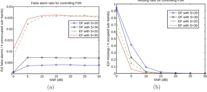
Figure 4.2: False alarm ratio vs missing ratio for controlling FSR with M = 100, K = 20,

λF SR = 4 and α = 0.05.

Figure 4.1(a) shows that both energy fusion and decision fusion can control the FSR under the desired level α while the proposed decision fusion method can achieve a much lower FSR level than the energy fusion. This improvement results from the discrete test statistics of the decision fusion and is proven as part of the theorem 5.1 in [11]. As it can be seen in Figure 4.2(a), controlling the FSR also leads to hold the false alarm ratio

at low level, and the decision fusion method outperforms the energy fusion method as well as the FSR performance. The effect of the more capable cognitive users is shown in Figure 4.2(b) when the missing ratio decreases in the low SNR region. Here, the energy fusion method that uses the whole energy information has the advantage with lower missing ratio.

4.1.1

The Region of the Energy Threshold

Here we discuss the considerations for the threshold of the energy detector λ. Ac-cording to Equation (4.2), the p-values are a function of the energy threshold λ. Even the Nj and xj are also correlated with λ. Intuitively, there will be a region for setting

the energy threshold because the BH procedure is conducted at level α. If the smallest

p-value is greater than α, then all the p-values are greater than α as well. The BH

procedure then becomes ineffective. On the other hand, if the biggest p-value is smaller than α

M, it will also lead to a failure. However, the energy threshold region is still very

loose under this condition.

A tighter region of λ can be obtained if we take the single user’s sensing quality into account. Since the sub-bands are randomly chosen by the cognitive users, it may happen if a sub-band has only one observer. Under this situation, we should ensure that the p-value of that sub-band is still workable for the BH procedure. For this reason, the lower bound of λ is obtained by setting the p-value of the single observer channel to be smaller than the maximum BH procedure level α. i.e. e−λ _{≤ α. On the other side, the}

upper bound of λ is obtained by setting the p-value of the single observer channel to be larger than the minimum BH procedure level α

M. i.e. e−λ ≥ Mα. It can be easily shown

that the region of λ is

− ln(α) ≤ λ ≤ − ln(α

where M is the number of total null hypotheses.

4.2

False Ignorance Rate (FIR)

Although a low FSR can benefit the overall system throughput, Figure 4.2(b) indi-cates that it results in a high missing ratio at low SNR. The primary users then suffer from larger MAI. To maintain the primary users’ transmissions under a tolerable inter-ference level, controlling the false ignorance rate (FIR) seems to be a feasible option and is presented in this chapter.

Define the FIR as the expected proportion of the number of falsely ignored channels over the total number of channels which are declared unoccupied. Based on this defini-tion, the new two hypotheses for a sub-band j scanned by a secondary user i are now given by

H0 : Yi,j = Xi,j+ Ni,j

H1 : Yi,j = Ni,j

where H0 assumes that the sub-band is occupied and H1 assumes the sub-band is

unoc-cupied.

Unlike the FSR case, the observed energy |Yi,j|2 of the i-th secondary user to the

j-th sub-band have different exponential distributions depending on the different signal

strength under the null hypothesis H0. An ideal operating mode which assumes that

the fusion center has the SNR information of the cognitive users is proposed first. This assumption is made here to demonstrate the effect of controlling the FIR. We consider later a more practical case in which the fusion center is operated under a nominal SNR in the end of this chapter.

4.2.1

The Ideal SNR Mode

In this mode, the fusion center is assumed to have the perfect knowledge of SNRs from each cognitive user. Assume that Ni,j ∼ CN (0, 1) and Xi,j ∼ CN (0, q), with

q > 1. Conditioned on H0, Y = |Yi,j|2is a random variable with exponential distribution

denoted by Y ∼ E( 1

q+1). Denote PM as the probability of success (missing probability)

of the Bernoulli trial when each time a cognitive user makes his own decision, i.e.

PM = P r{|Yi,j|2 ≤ λ |H0, q} = P r{Y ≤ λ |H0, q}

= Z _λ 0 1 q + 1 e −_q+1y _dy = 1 − e−q+1λ (4.4)

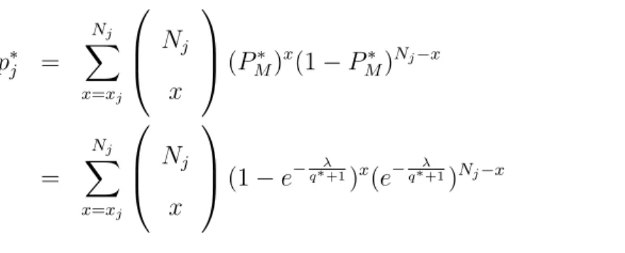
At the fusion center, the p-values of each sub-band are calculated by the CCDF of the Binomial distribution. pj = Nj X x=xj    Nj x    (PM)x(1 − PM)Nj−x (4.5) = Nj X x=xj    Nj x    (1 − e−q+1λ )x(e−q+1λ )Nj−x (4.6)

where Nj is the total number of decision bits in sub-band j and xj is the number of 0’s

in Nj.

Now, we apply the BH procedure at level α to detect the availability of the sub-bands as well. The steps are listed below.

1. Calculate each p-value pj, j = 1, 2, ..., M .

3. Find the largest index, imax, such that pimax ≤

imax

M α.

4. Declare sub-band j unoccupied for 1 ≤ j ≤ imax.

4.2.2

The Nominal SNR Mode

We consider here a more practical operating environment where the fusion center has no idea about the SNR information of each cognitive user. Instead of using the perfect SNR, a nominal SNR is set for the fusion center. We note that for each cognitive user, the decisions of the chosen sub-bands keep the same as the ideal SNR mode. Since the fusion center always operates at the nominal SNR, only the p-values of each sub-band are changed in this case.

Denote q∗ _{as the nominal SNR and P}∗

M as the probability of success corresponding

to q∗ _{at the fusion center. The expression of P}∗

M is obtained straightforwardly by

substi-tuting q∗ _{for q in (4.4). Besides, by substituting P}∗

M for PM in (4.6), the nominal p-value

for each sub-band denoted by p∗

j, j = 1, . . . , M , is also obtained. The equations for PM∗

and p∗

j, j = 1, . . . , M are given below respectively.

P∗

M = P r{|Yi,j|2 ≤ λ |H0, q∗} = P r{Y ≤ λ |H0, q∗}

= Z _λ 0 1 q∗_{+ 1}e −_q∗+1y _dy = 1 − e−q∗+1λ (4.7)

p∗_j = Nj X x=xj    Nj x    (PM∗ )x(1 − PM∗)Nj−x (4.8) = Nj X x=xj    Nj x    (1 − e−q∗+1λ )x(e− λ q∗+1)Nj−x (4.9)

Again, the BH procedure is applied to detect the availability of each sub-band based on the nominal p-values.

0 5 10 15 20 25 30 0 0.1 0.2 0.3 0.4 0.5 0.6 0.7 0.8 0.9 1 SNR (dB)

E(# false alarms / # unoccupied sub−bands)

False alarm ratio for controlling FIR

Ideal SNR S=30 Nominal SNR S=30 0 5 10 15 20 25 30 0 0.1 0.2 0.3 0.4 0.5 0.6 0.7 0.8 0.9 1 SNR (dB)

E(# missings / # occupied sub−bands)

Missing ratio for controlling FIR

Ideal SNR S=30 Nominal SNR S=30 FSR DF with S=30

(a) (b)

Figure 4.3: False alarm ratio vs. missing ratio for Ideal SNR mode and Nominal SNR mode with M = 100, K = 20, λF IR = 1, α = 0.05 and Nominal SNR = 10 dB.

As can be seen in Figure 4.1(b) and Figure 4.3, the ideal SNR mode obviously keeps the FIR under the desired level α and achieves a really low missing ratio at the same time. While it also makes the false alarm ratio at low SNR quite high, which is similar to what the missing ratio behaves in Figure 4.2(b) for FSR. However, to protect the primary users from large interference with low missing ratio is our major concern here. The nominal SNR mode is discussed below, and the fusion center is set to operate at

the nominal SNR = 10 (dB). Figure 4.3(b) and Figure 4.1(b) show respectively that the missing ratio increases in the SNR region lower than 10 (dB) and the FIR is also out of control in that region. In addition, the false alarm ratio becomes stable around 0.1 in Figure 4.3(a). Despite losing some control, the system seems to be operated under a good balance between the missing ratio and the false alarm ratio.

The reason why the nominal SNR mode behave in Figure 4.1(b) and Figure 4.3 is described here. When 0 ≤SNR≤ 10 (dB), the fusion center takes P∗

M which is greater

than the real PM as the probability of success for calculating the p-values of each

sub-band. Therefore a larger p-value is obtained than the ideal SNR mode which implies higher availability of the sub-band. The missing ratio then increases after applying the BH procedure. For SNR ≥ 10 (dB), since P∗

M is always smaller than the real PM, the

missing ratio will only be better than the ideal SNR mode. Note that P∗

M is fixed once

we set the nominal SNR at the fusion center. In order to compensate the effect caused by P∗

M, we should adjust the energy threshold to keep the missing ratio in an acceptable

Chapter 5

Application

In this chapter some applications are demonstrated to show the valuable extensions of the proposed cooperative sensing method. The first application is called ”The com-bined FSR and FIR approach”. In order to enhance the sensing performance, the BH procedures for controlling the FSR and the FIR are combined at the fusion center. The second application is called ”Detection of the signal strength in each sub-band”. By setting multiple hypotheses of different levels, we can estimate the signal strength in each sub-band after adopting the BH procedure. Since the BH procedure is a simple and low complexity multiple comparison procedure, it will not add much loading to the fusion center even if the BH procedure is applied more than one time.

5.1

The Combined FSR and FIR approach

The original inspiration of this application comes from the characteristic of the BH procedure. The BH procedure can ensure controlling the defined error rate but it does not control what is not defined. For example, as we can see at Chapter 4, the BH procedure controls the defined FSR under the given significance level and leads to a low false alarm ratio. However, the missing ratio is not the main concern at Chapter 4 so the performance is not quite satisfactory. The same situation can be seen when it turns

to the false alarm ratio in Section 4.2.1. If both the decisions of FSR and FIR are taken into consideration at the fusion center. We may have the advantages of the both sides.

5.1.1

Twice BH Procedure

To implement this application, we first change the single threshold energy detector into a two thresholds energy detector for obtaining the decisions bits of both FSR and FIR. The higher threshold is for controlling the FSR and the lower one is for controlling the FIR. When the observed energy of one sub-band exceeds the higher threshold, the cognitive user reports 1 for occupied channel . When the observed energy is below the lower threshold, it reports 0 for unoccupied channel. When the observed energy lies in between the two thresholds, it reports n for no decision.

At the fusion center, the BH procedure is tested twice to form the two reconstructive occupancy vectors, OF SR and OF IR . The first test of the BH procedure is conducted for

controlling the FSR. Equation (4.1) and (4.2) are used to calculate the p-values of each sub-band. The second test of the BH procedure is to control the FIR and the practical nominal SNR mode is adopted. Equation (4.7) and (4.9) can be employed here to obtain the p-values.

By comparing OF SR with OF IR, the final decisions of the availability of all the

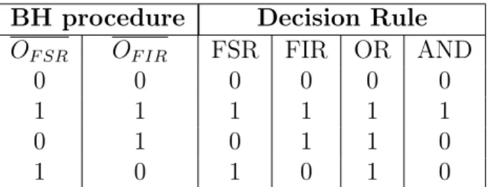
sub-bands are made. The possible decision rules are listed below.

BH procedure Decision Rule

OF SR OF IR FSR FIR OR AND

0 0 0 0 0 0

1 1 1 1 1 1

0 1 0 1 1 0

1 0 1 0 1 0

0 5 10 15 20 25 30 0 0.02 0.04 0.06 0.08 0.1 0.12 0.14 0.16 0.18 SNR (dB)

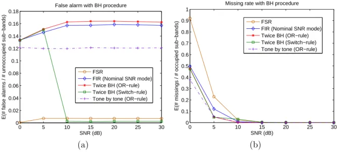
E(# false alarms / # unnoccupied sub−bands)

False alarm with BH procedure

FSR

FIR (Nominal SNR mode) Twice BH (OR−rule) Twice BH (Switch−rule) Tone by tone (OR−rule)

0 5 10 15 20 25 30 0 0.1 0.2 0.3 0.4 0.5 0.6 0.7 0.8 0.9 1 SNR (dB)

E(# missings / # occupied sub−bands)

Missing rate with BH procedure

FSR

FIR (Nominal SNR mode) Twice BH (OR−rule) Twice BH (Switch−rule) Tone by tone (OR−rule)

(a) (b)

Figure 5.2: False alarm ratio vs. missing ratio with M = 100, K = 20, λF SR = λh = 4,

λF IR = λl = 1, α = 0.05, Nominal SNR = 10 dB and Switching SNR = 5 dB.

5.1.2

The SNR Switching Rule

In order to protect the primary user from large MAI, we prefer not to use the sub-band when OF SR is different from OF IR (i.e. Using OR-rule). However, the missing

ratios in high SNR region shown in Figure 4.2(b) and Figure 4.3(b) are already low enough. Since the major concern of the missing performance is achieved, why don’t we turn to take care about the false alarm in this region? If we can somehow switch the decision rule between OR-rule and AND-rule based on whether the sub-band strength exceeds a threshold SNR. Then we can further improve our sensing quality. At last, we may achieve the goal for keeping both the false alarm ratio and the missing ratio at a considerably low level. In Figure 5.2, different decision rules are compared for their sensing performance. For SNR ≤ 10 (dB), the original FSR criterion has the best false alarm but the worst missing ratio. For decreasing the missing ratio, the FIR nominal SNR mode set at 10 (dB) is adopted by trading some false alarm ratio. The twice BH procedures can further reduce the missing ratio at SNR = 5 (dB) to the level equal to the tone-by-tone OR-rule. If we conduct the SNR switching rule at SNR = 10 (dB), both the false alarm and the missing ratios with SNR ≥ 10 (dB) are kept at a considerably

low level. The false alarm ratio for SNR ≥ 10 (dB) can achieve an even lower level than the original FSR criterion in Figure 5.2(a).

The SNR switching rule is proposed here for the win-win solution. The only problem here is that the fusion center needs to switch the decision rule once the sub-band signal strength exceeds the threshold SNR. For implementing this switching rule, another mul-tiple hypotheses testing problem is needed at the fusion center. Denote the threshold SNR as T h (dB), then the null hypothesis and the corresponding alternative hypothesis are stated respectively as below.

HT h : T he channel is occupied with signal strength at most T h dB

q∗ _{= 10}T h 10 (5.1) P_F∗ = Z _∞ λT h 1 q∗_{+ 1}e −_q∗+1y _{dy = e}−_q∗+1λT h _(5.2)

AT h : T he channel is occupied with signal strength at least T h dB

The BH procedure in Section 4.1 is applied here to test the above hypotheses for each sub-band. Since the null hypothesis is different from Section 4.1 now, the probability of success denoted as P∗

F is also changed. It can be easily calculated by (5.1) and (5.2).

Where λT h is the energy threshold applied to the local observations and is set at the

middle of the energy threshold region discussed at 4.1.1, i.e.

λT h = −(q∗+ 1) ln(α) + (

| − (q∗_{+ 1) ln(}α

M) + (q∗+ 1) ln(α)|

2 ) (5.3)

After applying the BH procedure, if the null hypothesis HT hof a sub-band is rejected,

it means that the signal strength in that sub-band is larger than the threshold SNR. Thus the switching rule can be implemented at the fusion center now. Based on the testing results, the fusion center then applies AND-rule to the sub-bands with HT h rejected and

5.2

Detection of the Signal Strength Region in each

Sub-band

After testing the signal strength in each sub-band to a threshold SNR in section 5.1.2, the method is further extended here to detect the precise signal strength region of each sub-band. This idea is motivated by [13]. The authors set several groups of hypotheses for detecting the number of signals embedded in noisy observations from a sensor array. After applying the BH procedure, the maximum null hypothesis rejected determines the lower bound of the number of signals.

In chapter 4, the hypotheses of one sub-band are only set for detecting the existence of the primary user. We don’t measure about the signal strength in each channel. However, if the fusion center has the knowledge of the signal strength, then the secondary users may not only transmit through the idle sub-bands, but also have chances to use the sub-bands in a more generic cognitive manner [14]. In [14], a CR system in which the secondary users can help transmitting the primary users’ data under the same channel is defined. Since the primary user has enough capability to fight the interference, it may allow the concurrent transmission of the secondary users under a acceptable level. By this way, the CR system can become more intelligent.

5.2.1

Decision Feedback Estimation

We call it Decision Feeaback Estimation (DFE) while the fusion center only uses the decision feedback bits to estimate the signal strength. At first, different hypotheses are assumed for different signal strength levels. These hypotheses are described as follows where H denotes the null hypotheses and A denotes the corresponding alternative hypotheses.

For L = noise,

Hnoise : T he channel is idle with only noise

q∗ _{= 0 (5.4)}

PF =

Z _∞

λnoise

e−ydy = e−λnoise _(5.5)

Anoise : T he channel is occupied with signal strength at least 0 dB

For L = 0, 5, 10, . . . , Lmax

HL: T he channel is occupied with signal strength at most L dB

q∗ _{= 10}L 10 (5.6) P_F∗ = Z _∞ λL 1 q∗_{+ 1}e −_q∗+1y _{dy = e}−_q∗+1λL _(5.7)

AL: T he channel is occupied with signal strength at least L dB

The notation Lmax represents the largest level of signal strength that is going to be tested

and P∗

F is the nominal probability of success going to be used by the BH procedure in

Chapter 4.

Note that here we consider the case in which each occupied sub-band will have an individual signal strength randomly chosen from {0 ∼ Lmax} (dB). For each level of

the hypotheses, the observers set different energy thresholds, λL, to test the observed

energy and report the one-bit decision bits. In order to set λL for each hypothesis level,

the middle values of the available energy threshold regions are used. According to the discussion in Section 4.1.1, the available region of each level can be easily obtained by the inequality below.

−(q∗_{+ 1) ln(α) ≤ λ}

L≤ −(q∗ + 1) ln(

α

Continuously, the BH procedure in Section 4.1 is adopted to test each signal strength level for obtaining the final decision pattern in each sub-band. There are two approaches to apply the BH procedure. One is called the horizontal approach and the other is called the vertical approach.

5.2.1.1 The horizontal approach

In this approach, the BH procedure is first applied repeatedly to test the M sub-bands for each signal strength level. The p-values which are going to be sorted are from different sub-bands. Since a single level result can only indicate that whether the sub-bands exceed the testing strength, the results of testing each signal strength level are needed here. After having all the results, the fusion center then decides the signal strength regions by the final decision pattern in each sub-band. The rules are given in (5.9).

5.2.1.2 The vertical approach

The vertical approach which does not test the M sub-bands at the same time uses the BH procedure to test the signal strength levels in a single sub-band. The p-values used here are calculated by the reporting bits from each strength levels. The signal strength region of a certain sub-band can be determined by the rules in (5.9) once the BH procedure is applied.

The estimation of the signal strength region in each sub-band q_j, j = 1, . . . , M is

determined by q_j =           

only noise if no H hypothesis is rejected

0 ∼ 5 dB if only Hnoise is rejected

L ∼ L + 5 dB if HL is the maximum rejected hypothesis

5.2.2

Energy Feedback Estimation

If the fusion center uses the whole energy feedback information to estimate the signal strength region, this method is called Energy Feedback Estimation (EFE).

Just like the DFE in 5.2.1, the hypotheses are set for testing different signal strength levels. Note that the EFE doesn’t need the probability of success PF or PF∗ which is

only used by DFE to calculate the p-values of each sub-bands. The p-values which only depend on the total observed energy in every sub-band are easily obtained by the CCDF of the gamma distributions. The hypotheses and the formulas for calculating p-values in EFE are listed below.

For L = noise,

Hnoise : T he channel is idle with only noise

q∗ = 0 (5.10)

pj = P r{Y ≥

X

|Yi,j|2 |Hnoise} = P r{Y ≥ Etotal |Hnoise}

= Z _∞ Etotal y(Nj−1)e−y Γ(Nj) dy, j = 1, . . . , M (5.11)

Anoise : T he channel is occupied with signal strength at least 0 dB

For L = 0, 5, 10, . . . , Lmax

HL: T he channel is occupied with signal strength at most L dB

q∗ _{= 1010}L _(5.12)

p∗

j = P r{Y ≥

X

|Yi,j|2 |HL, q∗} = P r{Y ≥ Etotal |HL, q∗}

= Z _∞ Etotal y(Nj−1)e−q∗+1y Γ(Nj)(q∗ + 1)Nj dy, j = 1, . . . , M (5.13)

AL: T he channel is occupied with signal strength at least L dB

also available here. The final decision rules for estimating the signal strength region is the same as (5.9).

Chapter 6

Simulation Results

Some numerical experiments are conducted to evaluate the proposed decision fusion method in this chapter. The simulation parameters are set as follows. Consider that there are M = 100 sub-bands going to be sensed by K = 20 users. Each channel is occupied by a primary user with equal probability, and each user can randomly select

S sub-bands to scan. Note that the energy threshold is set at λ = 4 for controlling the

FSR and is set at λ = 1 for controlling the FIR. Since the FSR and the FIR are tried to be controlled for two different concepts of CR systems, we should set appropriate energy thresholds for each one. The BH procedure is conducted at the level α = 0.05.

6.1

Cooperative Spectrum Sensing

At Chapter 4, there is an assumption that each occupied sub-band has a uniform signal strength according to the variance q of Xi,j. However, in practical communication

environments, this assumption is no longer true. Due to the possible fading or shadowing effects, the links between cognitive users and occupied sub-bands may have different channel conditions. There are three kinds of simulation environments going to be tested for cooperative spectrum sensing based on the BH procedure.

1. Sub-band Oriented Case (An idealized environment) :

An idealized environment is considered that each occupied sub-band has an indi-vidual signal strength. All cognitive users experience the same SNR in a sub-band. Since the signal strength is fixed in each sub-band, both FSR and FIR can be tested under this case. The probability of success and the p-values can be easily obtained by Equation (4.1), (4.2), (4.4), (4.6), (4.7) and (4.9). The most important part here is that the bases to sort p-values are different.

For reducing the calculation and showing the performance of the proposed decision fusion methods. This ideal case is assumed to simplify the environment. The SNR of each each occupied sub-band is randomly chosen from 0 ∼ 30 (dB).

2. Observer Oriented Case (An imaginary environment) :

An imaginary environment assumes that each cognitive user applies an uniform signal strength to all the sub-bands which are going to be scanned. Different users will have different signal strength. In this case, the decision bits in a single sub-band are based on varied level of observations. The ideal mode in Chapter 4.2 which needs the SNR information to calculate the p-values is not available now. However, controlling of the FSR and the nominal SNR mode for FIR can still be tested under this condition. The probability of success and the p-values can be easily obtained by Equation (4.1), (4.2), (4.7) and (4.9).

This case may apply to a situation where each user scans S consecutive sub-bands ,and these sub-bands have similar signal strength. e.g. a less frequency selective channel.

3. General Case (A practical environment) :

At last, the most practical communication environment is considered that each cog-nitive user experiences different signal strengthes in the sub-bands they scanned. This case is similar to the observer oriented case but the surroundings are more

complicated. Because of the same reasons as the previous imaginary environment, the ideal SNR mode for FIR is also unavailable. The probability of success and the p-values can be easily obtained by Equation (4.1), (4.2), (4.7) and (4.9).

5 10 15 20 25 30 35 0 0.02 0.04 0.06 0.08 0.1 0.12 0.14 S (sub−bands)

E(# false alarms / # unnoccupied sub−bands)

False alarm with BH procedure

FSR (General case) FSR (Sub−band oriented) FSR (Observer oriented) Tone by tone (General case)

5 10 15 20 25 30 35 0 0.05 0.1 0.15 0.2 0.25 0.3 0.35 0.4 0.45 0.5 S (sub−bands)

E(# missings / # occupied sub−bands)

Missing rate with BH procedure

FSR (General case) FSR (Sub−band oriented) FSR (Observer oriented) Tone by tone (General case)

(a) (b)

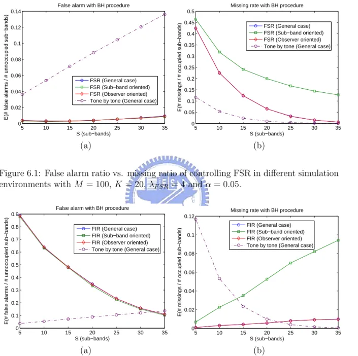
Figure 6.1: False alarm ratio vs. missing ratio of controlling FSR in different simulation environments with M = 100, K = 20, λF SR = 4 and α = 0.05.

5 10 15 20 25 30 35 0 0.1 0.2 0.3 0.4 0.5 0.6 0.7 0.8 0.9 S (sub−bands)

E(# false alarms / # unnoccupied sub−bands)

False alarm with BH procedure

FIR (General case) FIR (Sub−band oriented) FIR (Observer oriented) Tone by tone (General case)

5 10 15 20 25 30 35 0 0.02 0.04 0.06 0.08 0.1 0.12 S (sub−bands)

E(# missings / # occupied sub−bands)

Missing rate with BH procedure FIR (General case) FIR (Sub−band oriented) FIR (Observer oriented) Tone by tone (General case)

(a) (b)

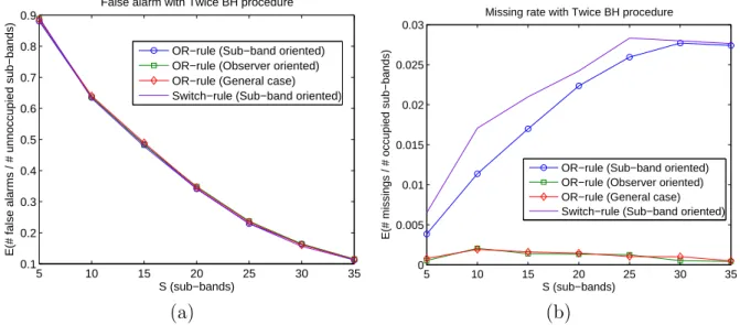
Figure 6.2: False alarm ratio vs. missing ratio of controlling FIR in different simulation environments with M = 100, K = 20, λF IR = 1, α = 0.05 and Nominal SNR = 10 dB.

The performance of the proposed cooperative sensing methods are discussed below. Note that here the common used OR-rule in narrow band spectrum sensing which

de-5 10 15 20 25 30 35 0.1 0.2 0.3 0.4 0.5 0.6 0.7 0.8 0.9 S (sub−bands)

E(# false alarms / # unnoccupied sub−bands)

False alarm with Twice BH procedure

OR−rule (Sub−band oriented) OR−rule (Observer oriented) OR−rule (General case) Switch−rule (Sub−band oriented)

5 10 15 20 25 30 35 0 0.005 0.01 0.015 0.02 0.025 0.03 S (sub−bands)

E(# missings / # occupied sub−bands)

Missing rate with Twice BH procedure

OR−rule (Sub−band oriented) OR−rule (Observer oriented) OR−rule (General case) Switch−rule (Sub−band oriented)

(a) (b)

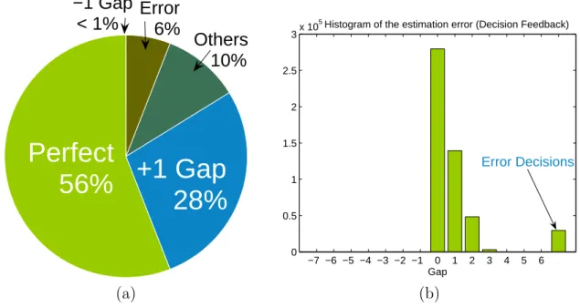
Figure 6.3: False alarm ratio vs. missing ratio of the twice BH procedure in different simulation environments with M = 100, K = 20, λF IR = 1, α = 0.05, Nominal SNR

= 10 dB, and Switching SNR = 5 dB.

clares channel occupied if more than one decision bits are 1 is applied to each sub-band for comparison. Figure 6.1 ∼ 6.3 show the false alarm and missing ratios under the three different simulation environments. For the FSR criterion, the false alarm ratios stay around 0.01 in all the environments and the missing ratios decrease with the in-creasing sub-bands per user can scan. For the tone-by-tone OR-rule, the false alarm ratio can’t be controlled because the probability to declare available sub-bands becomes less if there are more and more observers in one sub-band. The behavior that the missing ratio of the sub-band oriented case is higher than the other two environment settings in Figure 6.1(b) is caused by the fixed signal strength assumption. When a sub-band is experienced deep fading, the signal strength will be poor and last during that simulation trial, thus degrading the sensing performance. The same reasons can be also applied to the FIR criterion in Figure 6.2.

For the twice BH procedure, the OR-rule and the SNR switching rule are both simu-lated. Figure 6.3(b) shows that the OR-rule can decrease the missing ratio significantly compared with Figure 6.2(b) ,and the false alarm ratio still can be maintained at the

same level as Figure 6.2(a). In regard to the SNR switching rule, the threshold SNR is set at 5 (dB) based on the performance figure under uniform signal strength assumption in Figure 5.2(a). However, the SNR switching rule does not fulfill much of our expec-tation when applied to the sub-band oriented case in Figure 6.3(b). It reduces little false alarm ratio and enhances the missing ratio slightly at the same time. This may conflict with the original purpose of benefiting both false alarm and missing ratios but it remains a valuable approach for taking care of these two error ratios together.

6.2

Signal Strength Estimation

The performance of our signal strength estimation procedure is displayed by the pie charts and the histograms. The horizontal approach is showed in Figure 6.4 and 6.5 and the vertical approach is showed in Figure 6.6 and 6.7.

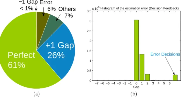
In this experiment, consider the channels are under the sub-band oriented case in which each occupied sub-band has an individual and fixed SNR randomly chosen from 0 ∼ 30 (dB). We separate the whole 0 ∼ 30 (dB) into several small non-overlapping SNR regions with each one of them 5 (dB) in width. After applying the rules (5.9) to the final decision patterns, the fusion center will then identify a SNR region for each sub-band. If the true SNR lies in the estimation region, the sub-band is called perfect estimation. The notation +1 Gap means that the true SNR is underestimated by one gap of the SNR region. Both horizontal and vertical approaches are tested for DFE and EFE respectively. The statistics are collected by testing 5 ∗ 105 _sub-bands.

−1 Gap

< 1%

Perfect

56%

+1 Gap

28%

Others

10%

Error

6%

Histogram of the estimation error (Decision Feedback)

Error Decisions

(a) (b)

Figure 6.4: The pie chart and the histogram of the Decision Feedback Estimation (DFE) under 5 × 105 _{sub-bands using horizontal approach.}

−1 Gap

< 1%

Perfect

67%

+1 Gap

28%

Others

2%

Error

3%

Histogram of the estimation error (Energy Feedback)

Error Decisions

(a) (b)

Figure 6.5: The pie chart and the histogram of the Energy Feedback Estimation (EFE) under 5 × 105 _{sub-bands using horizontal approach.}

−1 Gap

< 1%

Perfect

61%

+1 Gap

26%

Others

7%

Error

6%

Histogram of the estimation error (Decision Feedback)

Gap

Error Decisions

(a) (b)

Figure 6.6: The pie chart and the histogram of the Decision Feedback Estimation (DFE) under 5 × 105 _{sub-bands using vertical approach.}

−1 Gap

< 1%

Perfect

72%

+1 Gap

23%

Others

2%

Error

3%

Histogram of the estimation error (Energy Feedback)

Error Decisions

(a) (b)

Figure 6.7: The pie chart and the histogram of the Energy Feedback Estimation (EFE) under 5 × 105 _{sub-bands using vertical approach.}

First, the EFE shows a higher accuracy in the signal strength estimation for both horizontal and vertical approaches. This is the advantage of using the non-quantized energy information but it takes large transmission overhead for reporting. Although the DFE approaches have lower estimation accuracy, they can save the reporting bits while still achieving the accuracy around 85% combined the perfect with +1 Gap. The best estimation performance is the EFE of vertical approach with 72% being perfect estimates and 23% one scale higher. Besides, it also achieves a lowest 3% error rate. Noted that here the notation error in the pie charts means the proportion of the error decision sub-bands, i.e. the total number of false alarm and missing sub-bands. As you can see in Figure 6.4 ∼ 6.7, all of the four estimation procedures can achieve a low enough error rate with 6% and 3% respectively. Compare the horizontal approach with the vertical approach, it can be found that the vertical approach has better accuracy. Since the vertical approach applies the BH procedure to test the different levels of hypotheses inside a single sub-band, it can decide the signal strength independently without affecting by other sub-bands. However, the horizontal approach is used by applying the BH procedure to the different sub-bands for the same level of hypotheses. The conditions of other sub-bands may affect the decision results.

The histograms in Figure 6.4 ∼ 6.7 show the distributions of the estimation error. It can be found that the true signal strength is almost underestimate with a big part of +1 Gap. This characteristic can become the superiority for applying the SNR switching rule in the twice BH procedure because we have great confidence once the estimation strength exceeds the predefined threshold SNR. The characteristic may result from the conservative nature of controlling FSR. In Figure 4.2(a), it shows that controlling the FSR can leads to a low false alarm ratio at the same time ,and the events of false alarm in signal strength estimation here means that the estimation regions are higher than the true signal strength regions, i.e. the left side of the histograms. Since the four histograms all achieve the overestimation rate less than 1%, the proposed horizontal and vertical

Chapter 7

Conclusions

The decision fusion method was presented for cooperative spectrum sensing of wide-band cognitive radio systems using multiple hypotheses testing. Both FSR and FIR were defined based on the false discovery rate criterion and were shown to be controlled under a desired level by the BH procedure. Simulations showed that the decision fusion method can achieve a performance comparable to the energy fusion method while saving the overhead of reporting information. Moreover, the nominal SNR mode for a realistic operation was discussed. The results showed that the system seems to operate under a better balance between the missing and false alarm ratios by trading off some perfor-mance in the low SNR region. After introducing the SNR switching rule, the combined FSR and FIR approach performed the best and had both satisfactory false alarm and missing ratios. For estimating the signal strength, both EFE and DFE can achieve a low enough error rate of the availability of the sub-bands while the EFE showed a high accu-racy to the strength estimation. Although the DFE had worse accuaccu-racy, the true signal strength was almost underestimated. Compared to other spectrum sensing algorithms, our proposed methods have the advantages of wideband sensing, controllable error rates, lower complexities, and the ability for signal strength estimation. The overall sensing time and the average reporting bits can be further studied for future works.

Bibliography

[1] A. Ghasemi and E. S Sousa, “Collaborative spectrum sensing for opportunistic access in fading environments,” in Proc. 1st IEEE Symp. New Frontiers in Dynamic

Spectrum Access Networks. Baltimore, USA, Nov. 2005, pp. 131–136.

[2] C. Sun, W. Zhang, , and K. B. Letaief, “Cluster-Based cooperative spectrum sensing in cognitive radio systems,” in Proc. IEEE ICC. Glasgow, Scotland, Aug. 2007, pp. 2511–2515.

[3] C. Sun, W. Zhang, and K. B. Letaief, “Cooperative spectrum sensing for cognitive radios under bandwidth constraints,” in Proc. IEEE WCNC. Hong Kong, China, March 2007, pp. 1–5.

[4] G. Atia, E. Ermis, and V. Saligrama, “Robust energy efficient cooperative spectrum sensing in cognitive radios,” in Proc. IEEE SSP ’07. Madison, Wisconsin, Aug. 2007, pp. 502–506.

[5] S. Holm, “A simple sequentially rejective multiple test procedure,” Scand. J.

Statist., vol. 6, pp. 65–70, 1979.

[6] R. J. Simes, “An improved Bonferroni procedure for multiple tests of significance,”

Biometrika, vol. 73, pp. 751–754, 1986.

[7] G. Hommel, “A stagewise rejective multiple test procedure based on a modified Bonferroni test,” Biometrika, vol. 75, pp. 383–386, 1988.

[8] Y. Hochberg, “A sharper Bonferroni procedure for multiple tests of significance,”

Biometrika, vol. 75, pp. 800–803, 1988.

[9] D. M. Rom, “A sequentially rejective test procedure based on a modified Bonferroni inequality,” Biometrika, vol. 77, pp. 663–665, 1990.

[10] Y. Benjamini and Y. Hochberg, “Controlling the false discovery rate: A practical and powerful approach to mulitiple testing,” J. Roy. Statist. Soc. Ser. B, vol. 57, pp. 289–300, 1995.

[11] Y. Benjamini and D. Yekutieli, “The control of the false discovery rate in multiple testing under dependency,” The Annals of Statistics, vol. 29, no. 4, pp. 1165–1188, 2001.

[12] P.B. Gilbert, “A modified false discovery rate multiple-comparisons procedure for discrete data, applied to human immunodeficiency virus genetics,” Appl. Statist., vol. 54, Part1, pp. 143–158, 2005.

[13] P.-J. Chung, J. F. Bohme, C. F. Mecklenbrauker, and A. O. Hero, “Detection of the number of signals using the Benjamini-Hochberg procedure,” IEEE Transactions

on Signal Processing, vol. 55(6-1), pp. 2497–2508, July 2007.

[14] N. Devroye, P. Mitran, and V. Tarokh, “Achievable rates in cognitive radio chan-nels,” IEEE Transactions on Information Theory, vol. 52, no. 5, pp. 1813–1827, May 2006.