System design of orifice pulse-tube refrigerator using linear flow network analysis

(1)

PII: SOOll-2275(96)00064-l

System design of orifice pulse-tube

refrigerator using linear flow network

analysis

B.J. Huang and M.D. Chuang

Department of Mechanical Engineering, National Taiwan University, Taipei 10764, Taiwan

Received 4 September 1995; revised 5 March 1996

A linear flow network model was developed for the system analysis of an orifice pulse- tube refrigerator (OPT). The flow network analysis considers the pressure as the elec- tric voltage and the mass flow as the electric current. The linear governing equations for the flow network are derived from the continuity and the momentum equations and are analytically solved simultaneously with the energy equation derived to account for the thermal effect in the flow network. The thermal performance calculation can thus be greatly simplified by solving the equivalent circuit of the OPT using a sinusoidal signa_! analysis. To minimize the analytical errors, an equivalent pulse tube tempera- ture Tptm was introduced with a weighting factor W, which was determined experimen- tally. The linear flow network analysis provides a powerful tool for the system perform- ance analysis of an OPT. 0 1996 Elsevier Science Limited

Keywords: pulse-tube refrigerator; cryocooler; system analysis

Nomenclature

A Area (m*)

4 Cross-section area of piston (m*) 4 Flow area of connecting tube (m’)

A HT Regenerator matrix surface area (m2)

i:

Flow or thermal capacitance Frequency (Hz)

Convective heat transfer coefficient (W mm2 K-l)

k Thermal conductivity (Wm K-‘)

L How inductance (m-2)

:

Mass flow rate (kg s-l) Pressure (N m-*)

Ql_

Net cooling capacity (W)

R Gas constant (k.l kg-’ K-l); flow resistance (Pa s kg-‘)

s Laplace transform variable, complex number t Time (s)

T Temperature (K)

TH Pulse tube hot-end temperature (K) TI_ Cold-end temperature (K)

V0 Total volume of regenerator (m3) V,, Volume of cold space (m3)

Y

Kinematic viscosity of gas (m%) P Gas density (kg/m3)

7 Time constant (s)

W Angular frequency (rad/s)

Subscripts C Compression chamber ce Cold end f Gas; fluid F Flow g Gas h Hot-end exchanger Inlet t, Conduction m Matrix 0 Outlet

P Piston; constant pressure Pt Pulse tube

r Regenerator

S Solid; reservoir

t Connecting tube V Orifice; needle valve W wall

Greek letters Superscripts

E Porosity of regenerator matrix (dimensionless) - Perturbation

8 Phase angle (deg) Mean value

CL Viscosity of gas (N s/m2)

(2)

System design of orifice pulse-tube refrigerator: B.J. Huang and M.D. Chuang

A reliable CAD (computer-aided design) tool for the designer of an orifice pulse-tube refrigerator (OPT) is still not available. The engineer develops various kinds of OPT mainly by trial and error’-‘. This is due to the fact that the fundamental theory of OPT is not completely understood and the analytical skill is still not powerful enough.

A surface heat-pumping model was first used to interpret the phenomena of the basic pulse-tube refrigerator (BPT)‘. The enthalpy flow model using the phaser concept associ- ated with thermodynamic and heat transfer modelling was used to analyze the performance of an OPT9-14.

Since the physical phenomena inside an OPT involves complicated mass, momentum and heat transports at a transient state, analytic solutions of governing equations are almost impractical. Numerical analysis using the finite element method is also extremely difficult due to the large number of grids required and the numerical problemsr5. A supercomputer is thus needed. Moreover, the numerical analysis can only be carried out to analyze the OPT performance at a designated operating condition. An optimum design of the OPT refrigerator is thus not easily obtained. A thermoacoustic approach has been developed recently by many researchers 1c24 The thermoacoustic . phenomena of the working gas in an empty channel’G24 or a channel filled with regenerator matrix2s was used to explain the heat-pumping effect against the temperature gradient in the pulse tube. The longitudinal acoustic work flux (acoustic work energy) and the heat flux (heat energy) are defined. Energy conversion between the two fluxes along the gas- eous wave stream2’.24 is used to explain the heat pumping effect.

From the thermodynamic relation dH = dP/ptTdS and the enthalpy flow concept, it can be easily shown that the total energy flow is composed of an acoustic work flux (acoustic work energy) and a heat flux (heat energy)*(j. For acoustic heat transportation and energy transformation in an isothermal wall and an adiabatic wa1121-23, the acoustic work flux was interpreted as a result of the propagation of the pressure and velocity waves, while the heat flux is caused by the hydrodynamic transportation of entropy carried by the oscillatory gas velocity.

In practical applications, the conservations of mass, momentum and energy equations should be derived and solved first for the variables (pressure, temperature and velocity) in a thermoacoustic system. The energy flux fields as well as the acoustic work flux or heat flux can then be determined.

The basic equations for the thermoacoustic analysis of a sound oscillation in a channel were derived from the conservation principle of mass, momentum and energy”. Two- dimensional (2-D) equations were linearized and a set of longitudinal wave equations (in ordinary differential form) using complex variables were obtained. The solutions of the velocity and pressure fields from the wave equations were used to compute the acoustic work flux (acoustic power). The 2-D energy equations for the gas and the channel wall were solved separately with the heat transfer boundary conditions between gas and wall. The solution for the temperature field from the energy equation was used to compute the heat flux caused by the entropy transportation, i.e. the acoustic heat power.

The OPT refrigerator can be treated as a thermoacoustic oscillator. The cooling effect results from the interaction between the velocity (or mass flow) wave and the pressure (or temperature) wave. By a careful design, the heat-pump-

ing effect against the temperature gradient can be obtained in an OPT refrigerator21-23. For an OPT, it can be easily shown that the longitudinal total energy flux is the enthalpy flow within the pulse tube26 which can be expressed in the cycle-averaged form:

The enthalpy flow (jl)(=(rizC,n) within the pulse tube is actually the gross refrigeration power of a pulse tube refrigerator from which the system performance of an OPT can be calculated directly if the gas temperature field and the mass flow rate within the pulse tube are known. Equation ( 1 ), which is basically concluded from the equation of state of thermodynamics, was used to interpret the energy transport process within the pulse tube and the exchange between the work flow (work power) and the heat flow (heat power).

The analysis of OPT performance based on the thermoacoustic theory is much more complicated than for a sound wave in a simple channel. The development of the thermoacoustic model for the OPT refrigerator still suffers from a lack of analytical solutions. Finite difference solution of the wave equations of each component is required. For the system analysis of an OPT refrigerator, a successive numerical computation for each component is thus neces- sary. This is apparently not suitable for the development of a CAD tool for practical applications.

Another approach is developed in the present study from the viewpoint of system dynamics, instead of from the thermoacoustic viewpoint, although they have something in common. For the OPT refrigerator, the mass flow as well as the pressure and temperature of the working gas (helium) varies approximately sinusoidally due to the reciprocating motion (compression/expansion) of the piston*‘. Each component of the OPT such as the connecting tube, regenerator and pulse tube, etc., operates at a dynamic state. In terms of a system dynamics concept, each component is triggered by an input (physical force) and induces an output (physical response). The output in turn acts as the input of the adjacent downstream component. A linear dynamic model can be derived to describe the input/output relationship for each component by using the governing equations in conjunction with a linearization technique and some approximations.

Applying the electric circuit analogy, with voltage analogous to pressure and current analogous to mass flow rate, we can further obtain an equivalent circuit or block diagram for each component. Connecting the analogous circuits of all the components according to the orifice OPT process will lead to an analogous flow network of the system. For the OPT refrigerator, the equivalent circuit can be solved analytically, and the system performance evaluated.

The present approach will finally lead to a linear flow network model for the OPT. The flow network accounts mainly for the phenomena of the gas flow and the pressure variations. However, the energy equation is also solved simultaneously for the temperature distribution of gas as well as solid (regenerator matrix and pulse tube wall), from which the OPT performance can be calculated. Since the physical phenomena in an OPT are so complicated, any theoretical modelling will never be perfect. A modification based on the test results is thus needed. A modified flow network analysis is also proposed in the present study.

(3)

System design of orifice pulse-tube refrigerator: B.J. Huang and M.D. Chuang

System dynamics model of OPT

components

An orifice pulse tube refrigerator (Figure 1) consists of eight components, i.e. compression chamber, connecting tube, regenerator, cold space, pulse tube, hot-end heat exchanger, orifice and reservoir. The dynamics model of each component can be derived. For simplicity, the ideal gas assumption is used throughout the derivation in the present paper.

Compression chamber

A piston with reciprocating motion compresses the gas in the compression chamber and generates oscillating pressure and mass flow waves. Since the gas agitation is very severe, the gas temperature and pressure can be assumed to be uniform inside the compression chamber.

A dynamics models of the compression chamber is derived from the continuity equation with zero leakage between the piston and cylinder wall:

(2)

where riz, is the mass flow rate out of the compressor; P,

is the gas pressure; V,(t) = V,, - A&J t); V,, is the com-

pression s@ce volume for the piston at the equilibrium position with X, = 0; X,(t) is the piston displacement measured from the midpoint of the piston stroke toward the top dead end; and A, is the cross-section area of the piston.

Equation (2) is derived by assuming a constant gas tem- perature T,, i.e. an isothermal compression. This can hold approximately since efficient cooling is always provided for the compressor of an OPT. An order of magnitude analysis also shows that the effect on the mass flow rate riz, due to the rate of temperature rise, (P,V,/RT,2)dT,/dt, is relatively small compared to the effect due to the rate of pressure rise and the volume change rate in the compression chamber.

Applying a small perturbation around the equilibrium point (X,(t) = Xp + r?,(t); P,(t) = PC + PC(t); h,(t)

= r%, + k(t) = k(t)) to Ewation (2) neglecting higher- order terms, assuming that Xi, = 0 is the piston central position and then taking the Laplace transform, we obtain a perturbed dynamics model

A&) = iii,(s) +

sC,B,(s)

(3)

where c, = VJ(RT,); 7, = v,, -A&; &(s) = s&(~)

APFc/(RT,). The equivalent circuit for the compression

COMPRESSION CHAMBER

\ CONNECTING

I\\, \ I TUBE

chamber is shown in Figure 2 in which r&&s) acts as a current source representing the available or gross mass flow generated by the piston motion.

Connecting tube

The connecting tube links the compressor and the regenerator and a 1-D flow field is assumed. In order to obtain linearization, the second-order viscous term and the inertia term in the momentum equation are neglected. Second- order viscous friction is taken into account by a modified resistance coefficient K calculated using a piecewise linear approximation 15*17. Therefore, the viscous resistance is proportional to the mass flow rate with a proportional constant

K depending on the amplitude of the mass flow rate. The gas in the connecting tube is assumed

to

undergo an isothermal process with mean temperature T, which is

stationary. This usually holds since the connecting tube is usually small in diameter in order to reduce the system dead volume and has a thick wall in order to withstand the high gas pressure. Hence, the connecting tube can act as an energy storage medium to damp out the gas temperature variation easily.

From the above assumptions, we obtain the governing equations of the connecting tube from the conservation of mass and momentum.

1 dP(x,t) 1 dti(x,t)

RT, i% A, dx

1 &k&t) + aP(.&t) K .

A, at ax + pz(x,t) t = 0 (5)

It can be easily shown that Equations (4) and (5) can be converted into the form of wave equations.

Applying a small perturbation around the equilibrium point with _$z = 0 for a cyclically steady operation

(P(x,t) = P + P(x,t); & (XJ) = &+ riz(x,t) = rii(x,t)) to Equations (4) and (5) and then solving the Laplace trans- formed equations, we obtain the dynamics model of the connecting tube:

Figure 2 Equivalent circuit of compression chamber

COLD SPACE \ HOT-END HEAT EXCHANGER \ I I PULSE TUBE PISTON

Figure 1 Schematic diagram of an OPT refrigerator

(4)

System design of orifice pulse-tube refrigerator: B.J. Huang and M.D. Chuang

/

I[

13,0(s)

cosW,U

- Z,,sinh( r,L,)

**fi*o(s)**

=

- $

ct

sinh( r&J cosh(r&)

Ii I

IlltiCs)

pti(s)

(6)

where Tt = 6 and Z,, = G are the propagation constant and the characteristic impedance of the tube, respectively; Z, = RFt + sL,, = series impedance; and Y, = SC,, = shunt admittance; Tt and Z,, are derived as

rt = $GGG; Z,, = 2

Ft (7)

where CFt, L, and RFt are the flow capacitance, flow inductance and flow resistance per unit tube length, respectively, which are defined as

RFt=$;

C’Ft=$;

LFt=a

t _t t

From Roach and Bell’s experimental results for oscillating flow in a tube”,

K = 0.1556(~~~,,,d,l~)~~*~~(w~~~/~~) ₍₉₎

where w,,, is the peak velocity of the oscillating flow in the tube and d, is the hydraulic diameter of the tube.

It is worth noting that K is considered to be a constant during the modelling; however, it should be adjusted during the computation by numerical iteration to give a correct value for the corresponding mass flow (w,,).

Since the dynamic model of the connecting tube belongs to a distributed-parameter system, an equivalent circuit consisting of an infinite set of shunts and series impedances can be drawn as shown in Figure 3, which is based on the similar model of Equation (6) derived for N segments of the connecting tube 29 The shunt and series impedances . for each segment satisfy the following relations:

z,=zn+,=;zt

0

2

;z*=z3=...

=

z, = z,

0

5

N

Y*=Y*=Y,=...=Y,=Y,

0 $

₍₁₀₎

The limiting case, N+ 03, corresponds to the present model, Equation (6). The circuit can also be drawn based on the series expansion of cosh( r,L,) and sinh(r,&) in Equation (6) with respect to r,&29.

A system block diagram as shown in Figure 4 is used to illustrate the input/output relationship of the connecting tube from the system dynamics point of view.

Regenerator

The regenerator of an OFT is an energy-storage element made from wire mesh screen. The derivation of the dynamics model is similar to that of the connecting tube.

For the momentum equation, the inertia term (l/A~~)d(rizltillp)l&~ and the second-order viscous term

pp(ElpA,)%ltij can be neglected. This can hold since the Reynolds number in the regenerator is not large. The pressure loss due to second-order viscous friction is taken into account by a modified frictional coefficient h calculated using a piecewise linear approximationi5,i7. Therefore, the viscous resistance is assumed to be proportional to the mass flow with a proportional constant a which depends on the amplitude riz,, of the oscillating flow; ?% is considered to be a constant during the modelling; however, it should be adjusted by numerical iteration during the computation in order to give a correct value for the corresponding mass flow (riz,,).

Assuming 1-D flow, no axial conduction and constant properties, the transient governing equations in terms of perturbed variables (r;zlx,t) = k(x) + $x,t); P(x,t) = P,(x) + ~(x,t);T(x,t) = T,(x)+ T(x,t)) and noting g,(x) = 0 for cyclically steady operation are derived from the conservation of mass and momentum.

Continuity equation of gas

a&,t>

-

T,(x)-

-

P,(x)

at aF(x,t) + Rp drh(x,t) = o A ax (11)

fr

N m ti

Figure4 Block diagram of connecting tube

(5)

Momentum equation of gas

(12)

where R, is the regenerator flow resistance per unit length; LF, iS the flow inductance per unit length;

R, = -y; LFr = +

fr fr (13)

where a = cr + (~/d,&&,; cy = 175/( 2e&J, p = 1.6/(2&,,) can be obtained from Tanakas et al.‘s results3’; di, = hydraulic diameter = &l( 1-e); h = 0.33(kf/dh)R$f7 based on Tanakas et al.‘s results3’; and d, is the matrix wire

diameter.

For simplicity, the spatial variation of steady-state gas temperature-and pressure are approxima$ed by the average values, i.e. T,(x)=7’, = (TH+TL)/2 and P,(x)-P, = PC,,. It was experimentally justified that the temperature distribution in the regenerator of OPT is roughly linear.

Equations ( 11) and ( 12) cannot be solved since the gas temperature T(x,t) is not known. The following energy equations for the gas and the screen matrix are thus derived using the above approximation on T,(x) and p,(x).

Energy equation of gas

c,,

dP(x,t> + dh(x,t) CT, -

-at

Y ax +

y7gr

[T(G) -

~skt)l = 0

(14)

Energy equation of regenerator matrix

~~S.v>

7s

at + [Ts(x,t) - T(x,t)] = 0 (15)

where C,, and C,, are the how capacitance per unit length due to pressure and temperature change, respectively; rgr and r,, are time constants of gas and matrix, respectively, and y = CJC,; x is the position measured from the hot side of the regenerator;

c,, =

&

f’,&

ym

CT, =

RT2 ym

Pym~V&l

“I = RT,hA,,’

Ps(

l-•E)V&

rs, = hAm

(16)

where AHT is the surface area of the regenerator = 4V,( 1+)/d,,,; d,,, is the wire diameter of the screen disks; Reh is the Reynolds number based on dh; and kf is the gas

thermal conductivity.

Solutions of Equations (1 l), (12), (14) and (15) can be obtained by Laplace transform. Combining Equations (14) and (15) with (11) and (12), we obtain the gas continuity equation as

d&(x,s)

dx + sC,,P(x,s) = 0

and the gas momentum equation as

d&w>

dx + (RFr + sLF)&(x,s) = 0

where C,, is the regenerator flow capacitance due to pressure change and time responses of gas and matrix, which is derived as

c = c

1 +

7s

/[QA

l+%)l

FTr

FrY +

~sJ[~gr(1+~~s,)l

(19)

It is worth noting that Equations ( 17) and ( 18) have the form of wave equations.

A linearly perturbed dynamics model for the relationship between pressure and mass flow can be obtained’5z16:

[

II

~ro<s>

cosh( T,L,) -Z,,sinh( r,Lr)

fi,,(s) = - $sinh( I&.,) cosh( r,L,)

CT

(20)

where I, = @ = regenerator propagation constant and Z,, = fi = regenerator characteristic impedance; these are derived as

l-

r, =

JG-dRF,+~~F,);

Z, =

$

m-1

(21)

Similar to the connecting tube, the dynamics model of the regenerator belongs to a distributed-parameter system. An equivalent circuit consisting of an infinite series of shunt and series impedances can be drawn. This is based on the series expansion of cosh(r,L,) and sinh(rJ+) in Equation (20) with respect to T,L,. A system block diagram similar to Figure 4 can be drawn to show the input/output relationship from the system dynamics point of view.

The conservation equation of energy was also solved simultaneously using the solutions of P(x,s) and riz(Ls) to obtain the gas and solid temperatures. The gas temperature at the cold side of the regenerator (x = Lr,) is derived as

G Tgr( l+%,) - QLr,S) = - c _Pm(s) Tr rsr Y w+S7,,)r, 7 -- c,, s7

ST sinh(rA r

)[%(s)cosh(rrh) -

&its)1

(22)

This gas temperature solution T(L,,s) will finally be used with the mass flow solution $L,,s) to calculate the enthalpy flow out of the regenerator.

Cold space

The cold space is usually made of a small empty space, sometimes filled with a porous medium to enhance the heat transfer between the gas and the wall. The gas enters the cold space with phase difference between the temperature and the mass flow waves from which the refrigeration effect is generated. The gas agitation in the cold space is so severe that a uniform temperature in the cold space can be assumed. The mass accumulation rate due to the rate of change of gas temperature in the cold space is assumed to

(6)

System design of orifice poke-tube refrigerator: B.J. Huang and M.D. Chuang

be negligible since a high heat transfer between the cold- end exchanger (with large thermal mass) and the gas takes place. The mass continuity equation is thus derived as

7 7

vc,

@lx,

mcei -

mceo

=

RTc, dt (23)

Since pressure loss may also occur for gas flowing through the cold space, an approximate linear equation is used:

where R,, is the gas flow resistance through the cold space. The value of R,, can be obtained from empirical relations.

R,, can be neglected in OPT if the pressure loss in the cold

space is small compared to that in the regenerator. Equations (23) and (24) are solved to lead to a linearly perturbed dynamics model:

where C,, is the flow capacitance of the cold space defined as C,, = V,,/(RT,,). The equivalent circuit of the cold space is shown in Figure 5.

Pulse tube

The pulse tube acts as a resonant pipe for the gas flow and the pressure waves so that heat can be pumped from the cold space to the hot-side heat exchanger. Heat transfer between the gas and the tube wall exists and should be taken into account. For the momentum equation, the inertia term (l/A~,)~(riz~riz~lp)l~x and the second-order viscous term

(@pA$)hliizl can be neglected since the Reynolds number in the pulse tube is usually not very large. The pressure loss due to the second-order viscous friction is taken into account by a modified frictional coefficient u’ calculated using a piecewise linear approximation’5.17. Therefore, the viscous resistance is assumed to be proportional to the mass flow with a proportional constant u’ which depends on the amplitude ti,,, of the oscillating flow; (T’ is considered to be a constant during the modelling; however, it should be adjusted by numerical iteration during the computation in order to give a correct value for the corresponding mass flow amplitude (m,,,).

Similar to the regenerator modelling, the transient governing equations in terms of perturbed variables Lrit (x,t) = h,(x) + r&t); P(x,r) = P,,(x) + &x,t);T(x,t) =

T,,( x)+T(x,t)) with I;;(x) = 0 for cyclically steady operation are derived. The continuity equation for gas is

Figure 5 Equivalent circuit of cold space

dP(x,t) -

T,,(x)7

dF

RT;,(x)d& o - P,,(x)x +

Apt dx =

(26)

the momentum equation for gas is

1 a& aP U’V- p+z+ilm=O

Apt at Pt

(27)

u’ in Equation (27) is a corrected frictional parameter which will vary with flow rate and depend on the frictional factor of the pulse tube. It is found from Roach and Bell’s frictional factor for oscillating tube flowz8 that (T’ = 0.0389w,,, 0.7994L201 v-o.799

The spatial variation of the gas pressure at steady state p,,(x) can be approximated by the average value Pptm = _Pch. The spatial variation of gas temperature at steady state

Tpt(x) cannot be approximated by an average value since the gas temperature distribution in the pulse tube is not linear3’. We assume that T,,(xlcan be approximated by a weighted average temperature T,,, which is defined as

T,,(x) = T,,, = T, + K(Tn-T,) (28) where W, is a weighting factor accounting for the temperature effect-on the gas transport within the pulse tube. For

W, = 0.5, T,,, will become the arithmetic mean of T,_ and T H.

Through the above treatment, Equations (26) and (27) turn out to be linear. However, they still cannot be solved since the gas temperature FpL(x,t) is not known. The follow- ing linear perturbed energy equations for the gas and the screen matrix are thus derived.

Energy equation of gas

1 aB

~ ~RTpum ali;. + ~,T(x,t)-Ts(x,t)) = 0

~1 at + (r-l)A,, ax Apt (29)

Energy equation of pulse tube wall

~~s;,(x,t)

WCs

~ at + &,,A,[ Fs(x,t) - p(x,t)] = 0 (30)

MS is the mass of the tube per unit length; A, is the contact

surface area between the gas and the wall per unit length;

Apt is the gas flow area. The above energy equations are derived using approximation of Equation (28).

The heat transfer coefficient h,, in Equations (29) and (30) can be determined by using Tanaka et d’s results”‘:

h =

4.3WWpA

i

laminar flow Pi _{0.036(kfldpt)R,h0~8Pr”3(dpt/lpt)0~055,} _{turbulent flow}

(31)

R,, is the Reynolds number based on the inside diameter of the pulse tube.

Equations (26) (27), (29) and (30) then can be solved by Laplace transform. Combining the Laplace form of Equations (29) and (30) with that of Equations (26) and

(7)

(27), we obtain a linearly perturbed dynamics model for the pulse tube:

cosWptLpt) - ZcptsW~ptLpt)

I[ 1

IsptiCs) &tics)

(32) where rpt = _J-\iZ,,Y,, = sC~~~(&,~+SL~~J is the propagation constant of the pulse tube; Zcpt = Zpt/Ypt = r,dsC,,, is the characteristic impedance of the pulse tube; c FTpt is the flow capacitance due to a pressure change and time responses of the gas and tube wall which is derived as

c

F-rpt - - CF,,

1 + %pt47gpt(

l+s’Tspt)l

Y +

?pt4?gt( l+%pdl

(33)

RFpt is the flow resistance of the pulse tube per unit length;

C,,, is the flow capacitance per unit length due to the change in pressure; C,,, is the flow capacitance per unit length due to the change in temperature; and LFpt is the flow inductance per unit length; rgpt and rspt are the gas constants of gas and wall, respectively.

(34)

Similar to the regenerator, the dynamics model of the pulse tube belongs to a distributed-parameter system. An equivalent circuit consisting of an infinite series of shunt and series impedances can be drawn. This is based on the series expansion of cosh(rptLpt) and sinh(r,,L,,) in Equation (32) with respect to T,,L,,. A system block diag- ram similar to Figure 4 can be drawn to show the input/output relationships from the system dynamics point of view.

The gas and wall temperature distributions inside the pulse tube can be obtained by solving the energy equations of gas and wall using the solutions of P(W) and &((x,s). The gas temperature at the hot end of the pulse tube is derived as

CFpt Tgpt( 1 + WpJ -

T(L,,,s) = - 7 Ppds)

Tpf 7,pt

(35)

Hot-end heat exchanger

The major function of the hot-end heat exchanger is to reject heat to the surroundings. The hot-end heat exchanger is made of a tube connecting the pulse tube with the same diameter but filled with packed screen matrix to enhance the heat transfer between the gas and the wall. Since the hot-end heat exchanger is short and the heat transfer rate is large, it is assumed that the gas and the matrix tempera-

tures are uniform and identical at T,,. The energy equations are thus not needed in the modelling. The mass and momentum equations of the hot-end heat exchanger are basically the same as that of the regenerator. It then follows that the system dynamics model of the hot-end heat exchanger is

cosh(rhL)

-Z,,sinh( I,&,)

-

$sinh( r&J

I[ 1

pei(s>

cosh(ItJh)

A.ei(s)

ch

(36) where

rh = fi, zch

= a.

The definitions of Zh and Yh are similar to that in the regenerator.

Orifice

The orifice is used to provide a resistance for the flow between the pulse tube and the reservoir. By quasi-steady approximation, the pressure drop across the orifice can be expressed, in terms of the Laplace form of perturbation variables, as

pvo(s)

=

pvi(s>

- RF~&,(s)

(37)

where RFv is defined as the derivative of the pressure drop AP with respect to mass flow rate rit,. Since AP varies non- linearly with ti, and obeys the relation AP =

C@, + C,rit$ RFv is defined at a peak flow rate ti,,,, i.e. dAP

&v = dri? = c, + 2c$il,,, 0

%lax

(38)

RFv is considered to be a constant in the modelling, but it should be adjusted by numerical iteration during computation to give a correct value for the corresponding flow amplitude.

Equation (37) represents the system dynamics model of the orifice. The equivalent circuit is shown in Figure 6.

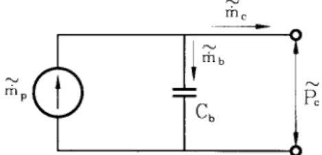
Reservoir

The reservoir is basically a large enclosed empty space act- ing as a damping device for the oscillating flow. Experi- mental evidence shows that the variation in gas temperature as well as pressure in the reservoir is small. Assuming a uniform and constant temperature T, in the reservoir, we obtain from the conservation of mass to the reservoir

@s(t)

Mt> = CFq-

(39)

Figure 6 Equivalent circuit of orifice

(8)

Figure 7 Equivalent circuit of reservoir

where C,, = V,I(RT,) is the flow capacitance of the reservoir; V, is the volume of the reservoir.

Applying linearization to Equation (39), we obtain a linearly perturbed dynamics model of the reservoir:

h,(t) = SC,,B,(S) (40)

The equivalent flow network circuit is shown in Figure 7.

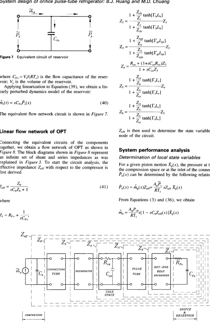
Linear flow network of OPT

Connecting the equivalent circuits of the components together, we obtain a flow network of OPT as shown in

Figure 8. The block diagrams shown in Figure 8 represent an infinite set of shunt and series impedances as was explained in Figure 3. To start the circuit analysis, the effective impedance Z,, with respect to the compressor is first derived where Z, = R,, + & FS (41) 1 + 2 tanh[r,&] z, = 1 1 + $ tanh[r,l,] Z, ch 1 + 2 tanh[ T,&,] z3 = 2 1 + $ tanh[ I’,&,,,] z2 CPt

z, =

Rce

+ ( l+sCceRcX,

1 + SC&

1 + 2 tanh[rJr] zs= 4 Z, 1 + 2 tanh[r,L,] CT 1 + 2 tanh[r&,] z,= 5 S 1 + 2 tanh[rJ,] Ct

Z,, is then used to determine the state variables at each node of the circuit.

System performance

analysis

Determination of local state variables

For a given piston motion xp(s), the pressure at the exit of the compression space or at the inlet of the connecting tube P,,(S) can be determined by the following relation:

From Equations (3) and (36), we obtain

(42)

-4

1 -

GGfwl~pb(~>

(43) 0 o-

1 R,

CONNECTING HOT-END I HEAT ORIFCE 1 RESh"OIR~

(9)

Combining Equations (6), (42) and (43), the pressure and the mass flow rate at the exit of the connecting tube, p&s) and r&, (s), respectively, can be determined. From Equa- tions (20), (25), (32), (36), (37) and (40), the pressure and mass flow rate at each node of the flow network can be determined. Finally, the gas temperatures at the cold end of the regenerator, F&L,,s)( =i;,,(s)), and at the hot end of the pulse tube, T&&,s)( =F&s)), can also be determined from Equations (22) and (35).

The state variables derived above are all in terms of transfer functions. For practical application, state variables in terms of time functions are needed for the calculation of thermal performance.

Since all the components of the OPT are triggered by the piston motion which is very close to sinusoidal, the variations of mass flow rate, pressure and gas temperature inside the OPT are assumed to be sinusoidal. This was justified experimentally3’m33. Therefore, by letting s = jw in the transfer functions, we obtain the Fourier-transform functions of the state variables. The successive computation is then greatly simplified by just using the amplitude and phase of each state variable. The results can easily be used to convert into the sinusoidal time function.

Net cooling capacity

To calculate the net cooling capacity of an OPT, an energy balance equation for the system should be derived first. Taking the control volume consisting of the cold space and the pulse tube (Figure 9), we obtain the cycle-averaged energy balance equation:

Q,_ = (f&t) - (ffr) - (Q,& - (Qk,rw) - (Qk,rrn)

(44) where QL is the net cooling capacity of the OPT; (Qk,,,) is the heat conduction loss of the pulse tube wall determined by

(Qk,pt> =

kptAwpt(Tpto

-

Tpti)

L Pl

(45)

where Awp, is the cross-sectional area of the pulse tube; (Qk,nv) is the heat conduction loss of the regenerator tube wall which is determined by

(QI& =

k,AA,(T,i-T,o)

L r

(46)

where A,, and k,, are the cross-sectional area and the thermal conductivity of the regenerator tube, respectively;

O-4)

-

Qk,rrn

Qk,rw COLD SPACE \ r--- /

(Qr_,) is the heat conduction loss due to the regenerator matrix:

(47)

where A, is the cross-sectional area of the regenerator matrix; k, is the effective thermal conductivity of the regenerator matrix. We have assumed that the tube wall temperature distributions of the regenerator and the pulse tube are linear. This may cause an error especially for the pulse tube and needs modification, as discussed later in this paper.

(H,,) is the cycle-mean or average enthalpy flow at the hot end of the pulse tube. (H,,) is calculated from the gas temperature F(L,,,t)( -Tp,,,( t)) and mass flow rate &c, at the hot end of the pulse tube using the relation for an ideal gas33,

(48)

where fImpto is the phase lead of the mass flow rate at the hot end of the pulse tube with respect to the piston motion; &rp, is the phase lead of the gas temperature at the hot end of the pulse tube with respect to the piston motion; r is the period of the piston motion; and C, is the heat capacity of gas at constant pressure.

(H,) is the average enthalpy flow at the cold end of the regenerator. (H,) is calculated using the following equation, for an ideal gas:

(H,) =

5

&,(t)~r,,(t) df 7

=

(49) where f3,,, is the phase lead of the mass flow rate at the cold end”of the regenerator with respect to the piston motion; OTTfr is the phase lead of the gas temperature at the cold end of the regenerator with respect to the piston motion.

The state variables determined previously can then be used to compute the average enthalpy flows, (HP,) and (I&), as well as the net cooling capacity QL of an OPT.

HOT-END

Ok,Pt _\ HEAT EXCHANGER _I

PULSE TUBE IFICE i /r-/////////////////,,,,,,,,,,,,,,,,~,,,, - --- 7--- REGENERATOR

_’

_QL

CONT\ROL VOLUME TUBE _WALL ‘QH

Figure 9 Control volume taken for net cooling capacity evaluation

(10)

System design of orifice pulse-tube refrigerator: B.J. Huang and M.D. Chuang System analysis procedure

To simplify the system analysis, the following assumptions are made

Since the gas in the compressor and the connecting tube is assumed to undergo a stationary and isothermal process, the regenerator inlet temperature T,i approximates to the_compression temperature T, and the connecting tube T,, i.e.

T,, = T, = T, (50)

The screen matrix in the hot-end heat exchanger provides a high heat transfer as well as large thermal inertia to the gas temperature. The inside gas temperature of the hot-end heat exchanger was assumed identical with the matrix temperature T,, and equal to the outside wall surface temperature TH, i.e.

T,, = T,, ₍₅₁₎

T,, is assumed to be stationary since the thermal mass of the hot-end heat exchanger is large.

The gas temperature in the cold space, T,,, is approxi- mately equal to the outside wall surface temperature of the cold end, TL. This was verified experimentally34 since the convective heat transfer between the gas and the wall in the cold space is very large, especially for low TL and a higher operating frequency; i.e.

T ce = TL (52)

TL is assumed to be stationary since the thermal mass of the cold-end exchanger is large compared to the gas inside the cold space.

The equilibrium value p for each perturbed pressure is assumed to equal the system charge pressure P,,. Since a solid tube wall usually has a large thermal mass and high thermal inertia, the wall temperatures at the two ends of the regenerator, T,,i and Tp,o, and at the two ends of the pulse tube, Tri and T,,, are approximately constant and stationary and obey the following relations

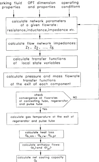
Given OPT dimensions and material physical properties, the operating conditions ( TL, TH, Pch,f, T,) and the working fluid properties, the system performance of an OPT can be carried out according to the flow chart shown in Figure 10.

Experimental

design

A single-stage orifice pulse-tube cooler was designed and built in the present study. The compression chamber is 28.58 mm in diameter, and 13 mm in stroke, with a swept volume of 6.8 cm3. The connecting tube was made from a stainless steel pipe of 1.75 mm inside diameter and 300 mm long. The regenerator is of 9 mm inside diameter, 67 mm long and packed with 720 disks of 200 mesh stainless steel wire screen. The pulse tube was made from stainless steel, with inside diameter 5.2 mm, 113 mm long and 0.15 mm wall thickness. The reservoir has a volume of 30 cm3. A

working fluid OPT dimension operating properties and properties conditions

i calculate network parameters

at a given flowrate:

resistance,inductance,impedance etc.

I t

calculate flow network impedances:

of local state variables

I

t

calculate pressure and mass flowrate transfer functions

at the exit of each component

1 I

check convergence 01 flowrates at connecting tube, ond pulse tube

1

calculate gas temperature at the exit of regenerator and pulse tube

Figure 10 Flow chart for performance analysis

needle valve is used to replace the orifice. The valve constants were determined experimentally as C, = 4.633 x lo9 Pa s kg-’ and C, = 2.238 x 1OL4 Pa s2 kgm2 at one turn. Helium gas with 99.999% purity is used as the working fluid.

Modification

of flow network analysis

Experimental verification of flow network analysis

The thermal performance prediction of an OPT using the present linear flow network analysis can be greatly simplified since the solutions of local state variables in transfer functions are obtained. Using sinusoidal signal analysis, the computation speed thus becomes very fast, taking a few seconds in a PC. However, the analytical results using the flow network analysis with W, = 0.5 are not accurate, as shown in Figure I I. This is probably due to the follow- ing factors.

1 The linearization and simplification of the governing equations may cause some errors, although a linear piecewise approximation has been taken to compensate the non-linear effect in the evaluation of the flow resistance in the connecting tube, the regenerator and the pulse tube.

(11)

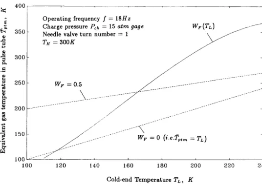
Operating frequency f = 18Hz Charge pressure Pch = 15 atm gage Needle valve turn number = 1 TH = 300K

calculated with WF

100 150 200 250

Cold-end Temperature TL , K

Figure 11 Comparison of flow network analysis and test results

of the energy equations of the pulse tube as a constant value. In Figure 11, we take equal weighting, i.e.

W, = 0.5, which implies T,,, = (TL+TH)12.

Some other unmodelled effects such as real gas, temperature variation of gas and solid material properties, and gas heat conduction along the flow direction, etc., may cause errors.

The sinusoidal signal assumption within the OPT may deviate slightly from the actual signals, as was observed experimentally33.

The empirical correlations of the flow resistance and the convective heat transfer coefficient taken in the present analysis for oscillating flow in the connecting tube, the regenerator and the pulse tube may not be accurate. Among all the above possible factors, the second one is probably the dominant factor. An empirical modification on T,,, is thus considered in the present study.

Modification of flow network analysis

In order to linearize the continuity and energy equations of the pulse tube, the steady-state gas temperature within the pulse tube T,,(x) is gproximated by T,,,, the weighted average temperature. T,,, is defined with the weighting fac-

tor WF, i.e.

T,,, can be considered as the gas equivalent temperature within the pulse tube which affects the local variation in mass and enthalpy flows. Since the axial gas temperature distribution within the pulse tube is not linear and varies with the operating conditions such as TL, TH, PC,,,

f,

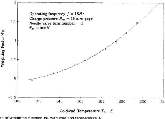
etc., using equal weighting (W, = 0.5) will cause a larger error. To modify the flow network analysis, we therefore con- sider the weighting factor W, to be a function of the cold- end temperature TL, instead of a constant, for a given charge pressure PC,, and operating frequency f, i.e. W&T,).

The functional relationship will be determined by matching the analytical results with the test data:

W, = 0.6217 - O.O1638T,_ + 9.433 x 10m5Tt (TL in K) (53)

Figure 12 shows the variation in W, with TL. Using the above empirical function W,(T,), the analysis is improved as shown in Figure 13.

Figure-14 presents the variation in the equivalent tem- perature T,,, with TL, using a constant W, or the above

function W,( TL). For zero weighting W, = 0, the equivalent temperature is just th_e cold-end temperature TL, For equal

weighting W, = 0.5, T,,, is the arithmetic mean of T,_ and T,, i.e. (TL+TH)12. In this case, the net cooling capacity QL

is overestimated at low TL and underestimated at high TL, as shown in Figure II.

The negative value of W, indicates that T,,, is lower than the cold-end temperature TL. This does not happen very

often and is probably caused by the simplification and linearization of the pulse-tube model. The small negative value of W, around zero cooling capacity ( QL = 0) shown in Figure 12 is probably just the computation error.

Experimental results indicate that the weighting factor depends not only on TL, but also on the charge pressure

P,, and the operating frequency J An empirical relation was concluded from a large number of test results:

W,(T,, Pch,fl = [6.63 x 10-5T;

+ 2.833 x 10-3TL - I.0231

x [0.0163Pzh + 0.34Pch - 2.161

x [5.40 x 10m3f2 - 0.286

f +

2.161 (54) where TL is in K, PC,, in atm abs and f in Hz.

The system design analysis of an OPT using the above empirical relation gives more than 85% confidence. That is, more than 85 out of 100 designs are accurate, with an error less than 10 K on the T,_ prediction at a given QL.

(12)

1

,.-

Operating frequency f = 18Hr /’

Charge pressure PC,, = 15 atm gage /’

Needle valve turn number = 1

,P / TH = 300K _I -0.5 2 100 120 140 160 180 200 220 240 Cold-end Temperature TL , K Figure 12 Variation of weighting function W, with cold-end temperature T,

TM = 300K 5- - Calculated with WF(TL) o Experiment II___ 4- /” / 0 3- / / 0 100 120 140 160 180 200 Cold-end Temperature TL , K 220 240

Figure 13 Prediction of cooling capacity using flow network analysis with empirical W,

Discussion and conclusions

From conventional electric circuit analogy, the flow network analysis considers the pressure as the electric voltage and the mass flow as the electric current. The governing equations of the flow network analysis are thus derived solely from the continuity and momentum equations. How- ever, the solutions for the flow network model cannot be found without the temperature solution since the effect of temperature variation is involved in the governing equations of the flow network of an OFT. Consequently, the thermal performance of an OFT cannot be evaluated since the gas temperature at the cold end of the regenerator is not known. This is why earlier thermoacoustic analysis can only discuss the fluid motion in a homogeneous tem-

perature field and the thermal performance calculation for the OPT was very difficult.

The present approach first derives the linear flow network equations in the form of wave equations. The linear energy equations were also derived and solved simultaneously in conjuction with the flow network equations. The energy equations for the regenerator and the pulse tube, including the gas phase as well as the solid phase (regenerator matrix and pulse-tube wall), take into account the heat transfer process between the gas and the regenerator matrix or the pulse-tube wall. The gas transport within the regenerator and the pulse tube is thus treated implicitly as an irreversible process from the viewpoint of thermodynamics.

(13)

System design of orifice pulse-tube refrigerator: B.J. Huang and M.D. Chuang

Q 400

z Operating frequency f = MHz

kg _{350 -} Charge pressure PC,, = 15 atm gage WF PL)

d

Needle valve turn number = 1

TH = 300K \ 2 d 2 300 - /’ 100 120 140 160 180 200 220 240 Cold-end Temperature TL, K

Figure 14 Equivalent gas temperature in pulse tube

time, s

Figure 15 Variation of gas temperature and mass flow rate at cold end of regenerator (the i,,, lead R by 36.03”; the r$, lead A,, by 74.6’)

erning equations as well as the energy equations are

employed in the present study. This finally results in a set of linear equations which are analytically soluble. The thermal performance calculation can then be greatly simplified by using sinusoidal signal analysis.

The analytical errors caused by the simplifications need further modification. The gas temperature effect in the pulse tube is considered-to be dominant and an equivalent pulse tube temperature Tptm was defined with a weighting factor W, which was determined experimentally. Since the performance calculation of an OPT becomes very simple and fast by using the present flow network model and sinusoidal signal analysis, W, can easily be determined for various operating conditions if the test results are available.

The linear flow network analysis provides a powerful tool for the system performance analysis of an OPT. It can be easily implemented for the performance calculation of an OPT by sinusoidal signal analysis. The accuracy of the present analysis, however, depends on the weighting factor W,. The derivation of an empirical relation for W, covering a wide range of design specifications and operating conditions is thus quite crucial in the development of the present linear flow network analysis for the OPT design. It relies mainly on experience. The empirical relation of equation (54) gives a design confidence higher than 85%. To further improve the accuracy, we are developing an expert system with learning capability in order to find W, more accurately.

(14)

It should be pointed out that the present linear flow network analysis also determines the spatial variation of state variable (mass flow rate, pressure and gas and solid temperature) in the OPT. The time variations of the gas temperture, i;,(t), and the mass flow rate, &,(t), at the cold end of the regenerator are predicted and shown in

Figure 1.5. The amplitude and phase shift of every state variable at various locations can also be calculated.

With these solutions and the equation of state of the working gas, the local acoustic power (or work flow) as well as the local heat power (or heat flow caused by entropy transportation) expressed on the right-hand side of Equ- ation ( 1) can also be evaluated. The calculations are omitted here since it is not the main theme of the present paper. The cycle average enthalpy flows, (H,) and (Hpt), in Equation (44) can be divided into two terms (work flow and heat flow) and computed. Detailed calculation of the work (or acoustic) and heat power in the pulse tube is also omitted since it is beyond the major scope of the present paper.

Finally, the present study indicates that the OPT design using the linear flow network analysis is feasible and better than the other methods. The accuracy of the system design of an OPT refrigerator using the linear flow network analysis can be further improved if a better empirical correlation of W, is obtained. This can be gradually achieved by accumulating more test results on various OPT refrigerators and updating the correlation. In the present study, the OPT is basically treated as a dynamic system with a flow network. The flow network analysis can then be used to further investigate the system performance as well as optimization according to the circuit behaviours.

Acknowledgement

The present study was supported by the National Science Council, Taiwan, ROC, through Grant No. NSCSl-0401- E002-587 and Grant No. CS83-0210-D002-011.

References

Zhu, S., Wu, P. and Chen, Z. Double inlet pulse tube refrigerators: an important improvement Cyrogenics (1990) 30 514-520 Wang, C., Wu, P.Y. and Chen, Z.Q. Numerical analysis of double- inlet pulse tube refrigerator Cryogenics (1994) 33 526-530 Cai, J.H., Wang, JJ., Zhu, W.X. and Zhou, Y. Experimental analysis of the multi-bypass principle in pulse tube refrigerator Cryogenics

(1994) 34 713-715

Wang, C., Wu, P.Y. and Chen, Z.Q. Modified orifice pulse tube refrigerator without a reservoir Cryogenics (1994) 34 31-36 Wang, J., Zhu, W., Zhang, P. and Zhou, Y. A compact co-axial pulse tube refrigerator for practical application Cryogenics (1990) 30

September Supplement (ICEC 13 Proceedings) 267-271

Richardson, R.N. Development of a practical pulse tube refrigerator: co-axial design and the influence of viscosity Cryogenics (1988) 28 516-520

Kurlhama, T., Hatakeyama, H., Ohtani, Y., Nakagome, H., Mat- subara, Y., Okuda, H. and Murakaml, H. Development of pulse tube refrigerator with linear-motor drive compressor Proc 7rh Int Cyrocooler Conf Vol 1, Sante Fe, NM, USA, 17-19 November

8 9 10 11 12 13 14 15 16 17 18 19 20 21 22 23 24 25 26 27 28 29 30 31 32 33 34

(1992) published by Philips Lab., Report No. PL-CP-93-1001 (1993) 157-165

Gifford, W.E. and Longsworth, R.C. Surface heat pumping, Adv Cryog Eng (1965) 11 171-179

Starch, P.J. and Radebaugh, R. Development and experimental test of an analytical model of the orifice pulse tube refrigerator Adv Cryog Eng (1988) 33 851-859

Radebaugh, R. A review of pulse tube refrigerator Adv Cryog Eng (1990) 35 1191-1205

Baks, M., Hirschberg, A., van der Ceelen, B. and Guijsman, H.M. Experimental verification of an analytical model for orifice pulse tube refrigeration Cryogenics (1990) 30 947-95 1

Harpole, G.M. and Chan, C.K. Pulse tube cooler modeling Proc

6th Znt Cyrocoolers ConJ Vol 1 Plymouth, MA, 25-26 October (1990) 91-101

Mirels, H. Linearized pulse tube cryocooler theory Proc 7th Int

Cryocoolers Co& Vol 1 , Sante Fe, NM, (1992) 221-232 Zhu, S.W. and Chen, Z.Q. Isothermal model of pulse tube refriger- ator Cryogenics (1994) 34 591-595

Harpole, G.M. and Chan, C.K. Pulse tube cooler modeling Proc

6th Znt Cryocooler Conf Vol 1, Plymouth, MA ( 1991)

Swift, G.W. Tbermoacoustic engines J Acoust Sot Am (1988) 84 1145

Luck, H. and Trepp, C. Thermoacoustic oscillations in cryogenics. Part 1: Basic theory and experimental verification Cryogenics (1992) 32 690-697

Luck, H. and Trepp, C. Thermoacoustic oscillations in cryogenics. Part 2: Applications Cryogenics (1992) 32 698-706

Luck, H. and Trepp, C. Thermoacoustic oscillations in cryogenics. Part 3: Avoiding and damping of oscillations Cryogenics (1992) 32

703-706

Xiao, J.H. Thermoacoustic effects and thermoacoustic theory for regenerative cryocoolers (heat engines) PhD Dissertation Institute of Physics, Academia Sinica, China (1990) (in Chinese)

Xiao, J.H. Thermoacoustic heat transportation and energy transformation. Part 1: Formulation of the problem Cryogenics (1995) 35

15-20

Xiao, J.H. Tbermoacoustic heat transplantation and energy transformation. Part 2: Isothermal wall thermoacoustic effects Cryogenics (1995) 35 21-26

Xiao, J.H. Tbermoacoustic heat transportation and energy transformation. Part 3: Adiabatic wall tbermoacoustic effects Cryogenics

(1995) 35 27-30

Tominaga, A. Thermodynamic aspects of tbermoacoustic theory Cryogenics (1995) 35 427-440

Xiang, Y., Kuang, B. and Guo, F.Z. Parity simulation of thermoacoustic effect in regenerator of Stirling cryocooler Cryogenics ( 1995) 35 489-494

Rawlins, W., Radebaugh, R. and Bradley, P.E. Energy flows in an

orifice pulse tube refrigerator Adv Ctyog Eng (1994) 39 1449-1456

Kral, S.F., Hill, D., Restivo, J. and Johnson, J. Test results of an

orifice pulse refrigerator Adv Cryog Eng (1992) 37 (Part B) 931-937

Roach, P.D. and Bell, KJ. Analysis of pressure drop and heat trans-

fer data from the reversing flow test facility, Argonne National Lab- oratory Report ANL/MCT-88-2 (May 1989)

Lo, T.C. Now Network Theory Mechanical Industrial Pub. Inc., Beij-

ing (1988) (in Chinese)

Tanaka, M., Yamashita, I. and Chisaka, F. Flow and heat transfer

characteristics of Stirling engine regenerator in an oscillating flow

JSME Znt J Series ZZ ( 1990)

Rawlins, W., Timmerhaus, K.D. and Radebaugh, R. Measurement