An Efficient Variable Partitioning and Scheduling Algorithm for DSP with Multiple Memory Modules

全文

(1)Int. Computer Symposium, Dec. 15-17, 2004, Taipei, Taiwan.. An Efficient Variable Partitioning and Scheduling Algorithm for DSP with Multiple Memory Modules Yi-Hsuan Lee and Cheng Chen Department of Computer Science and Information Engineering 1001 Ta Hsueh Road, Hsinchu, Taiwan, 30050, Republic of China Tel: (8863) 5712121 EXT: 54734, Fax: (8863) 5724176 E-mail: {yslee, cchen}@csie.nctu.edu.tw applications [3-4]. Since data are partitioned to. Abstract Multiple on-chip memory modules are attractive. separate memory banks and accessed simultaneously,. to many DSP applications. This architectural feature. this architecture offers higher memory bandwidth and. supports higher memory bandwidth by executing. performance potentially. However, its performance. multiple data memory accesses in parallel. However,. gain strongly depends on variable partitioning and. the performance gain in this architecture strongly. scheduling techniques [4].. depends on the variable partitioning and scheduling. The variable partitioning and scheduling problem. method. In this paper, we propose an efficient. is proven to be NP-complete. Rotation scheduling. rotation scheduling with parallelization (RSP), which. with variable repartitioning (RSVR) is an effective. is extended from our previous studies. RSP includes a. heuristic [4], and we propose two algorithms before. simple mechanism to partition variables, and uses. [5]. In this paper, we design rotation scheduling with. rotation scheduling and unimodular transformations. parallelization (RSP) by integrating unimodular. to generate effective results. We also design an. transformations technique. An analytic model and. analytic model to analysis preliminary performances.. DSP applications are used to evaluate preliminary. Based on our analyses, RSP can obtain quite effective. performances. From our analyses, RSP is quite. results compared with related methods.. effective compared with related methods. The remainder of this paper is organized as. 1. Introduction. follows. Section 2 describes the problem modeling. Most scientific and digital signal processing (DSP). and related work. Design issues and principles of RSP. applications, such as image processing and weather. are introduced in Section 3. Section 4 contains the. forecasting, are iterative and usually represented by. analytic model and preliminary analyses. Finally, we. uniform nested loops [1]. Digital signal processor is a. give some conclusions in Section 5.. special-purpose microprocessor, which is designed to achieve high performance on DSP applications.. 2. Unlike general-purpose CPU, the DSP is designed on. 2.1. Harvard architecture, and often includes independent. Fundamental Background Modeling the Given Program [4-5] Multi-dimensional data flow graph (MDFG). function units which can operate in parallel [2].. defined below is widely used to represent uniform. The growing gap of speed between CPU and. nested loop in previous researches. Nodes in the. memory becomes one of the most critical problems. MDFG can be both ALU operations and memory. for high-performance systems design. Thus, multiple. operations. Figure 1(a)(b) shows an nested loop and. on-chip memory modules are attractive to many DSP. its MDFG.. 1320.

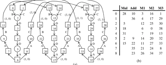
(2) Int. Computer Symposium, Dec. 15-17, 2004, Taipei, Taiwan. 0. for i = 1 to m for j = 1 to n D[i, j] = B[i-1, j] × C[i-1, j-2] ; A[i, j] = D[i, j] × 0.5 ; B[i, j] = A[i, j] + 1 ; C[i, j] = A[i, j-1] + 2 ; end end. B. (1, 0). 0. 1 C 2. (1, 2). (1, 1). 12. 11. D. 11. 1. B. C D. B. C 4 D. A 5. 7. B. 10. 9. A. A. 8. C 4. 6. 10 D. 5. 7. A. (a). 12. 3. 3. 9. (3, 1). 2. A 8. A (0, 1). (b). ALU operation memory operation. 6. (1, 0). (c). Figure 1. (a) Nested loop, (b) corresponding MDFG, (c) parallelized MDFG. Definition A multi-dimensional data flow graph. executed to complete the process. Usually, the time. (MDFG) G = (V, E, X, d, t) is a node-weighted and. required for prologue and epilogue are negligible.. edge-weighted direct graph, where V is the set of. 2.3. Unimodular Transformations Technique [8]. computation nodes, E is the edge set of precedence. Loop transformation is one of basic techniques. relations, X(e) represents the variable accessed by an. for parallel compiler design. It changes the execution. edge e, d(e) is the delays between nodes, and t(v) is. sequence of iterations to achieve higher degree of. the computation time of node v.. parallelism. Unimodular transformations technique. A MDFG is realizable if there exists a schedule. unifies loop permutation, skewing, and reversal, and. vector s such that s•d ≥ 0, where d are loop-carried. models them as elementary matrix transformations.. dependencies [6]. An iteration is equivalent to. All combinations of these loop transformations can. execute each node in V exactly once. The period. simply be represented as products of the elementary. during which all nodes in an iteration are executed. transformation matrices.. without resource constraints is called a cycle period.. 2.4. Related Work. Cycle period is the maximum computational time. Since retiming is useful for generating compact. among paths that have no delay, which will dominate. schedules, many scheduling algorithms are designed. the entire execution time of a nested loop.. based on it. In order to solve the variable partitioning. 2.2. and scheduling problem, Rotation scheduling with. Retiming Technique [7] Retiming is a technique that redistributes nodes in. variable repartitioning (RSVR) [4], modified from. consecutive iterations to enhance the performance.. rotation scheduling by considering multiple memory. n. The retiming vector r(u), a function from V ot Z ,. modules while constructing a schedule, is proposed.. represents the offset between the original iteration. RSVR uses variable independence graph (VIG) to. and that after retiming. A MDFG Gr = (V, E, X, dr, t). partition variables initially. When the schedule length. is created after applying r such that each iteration still. cannot be improved in a rotation phase, it will try to. has one execution of each node. Delay vectors will be. repartition variables to shorten the schedule length.. changed accordingly to preserve dependencies.. We have proposed rotation scheduling with. A prologue is the instruction set that must be. unfolding (RSF) and rotation scheduling with tiling. executed to provide data for the iterative process. An. (RST) for the same problem before [5]. RSF and RST. epilogue is the complementary set that will be. use simpler variable partitioning mechanisms, and. 1321.

(3) Int. Computer Symposium, Dec. 15-17, 2004, Taipei, Taiwan. Input: MDFG G = (V, E, X, d, t), N Output: schedule S 1. Allocate variables to N memory modules 2. Gp = parallelize G that the inner loop is parallelizable 3. GN = unfold GP with factor N 4. Select the schedule vector s = (1, 0) 5. S = schedule GN using list scheduling 6. S’ = compact S using rotation scheduling 7. Return S’. Input: MDFG G = (V, E, X, d, t) Output: MDFG G’ = (V, E, X, d’, t). 1. T = 1 0 ; G’ = G; 0 1   . 2. while (∃ (a, 0) and (b, 0) in d’, for a, b > 0) T = T × 1 0 ; ∀ d’(e) ∈ d, d’(e) = T × d’(e); 1 1  . 3. if (∃ (a, 0) in d’, for a > 0) (a) if (∃ (b, -c) in d’, for b, c > 0) T=T× . 1 0 ;  (c + 1) b 1   . Figure 3. The scheduling steps of RSP. partitioning mechanism and loop parallelization. (b) T = T × 0 1 ; ∀ d’(e) ∈ d, d’(e) = T × d’(e); 1 0  . algorithm in detail. Scheduling steps of RSP will be listed in Section 3.4. Since nested loop used in DSP. 4. Return G’ = (V, E, X, d’, t). applications are usually with depth two, we use the. Figure 2. Loop parallelization algorithm.. two-dimensional MDFG to design and analysis RSP. don’t need to repartition variables during rotation. However, RSP and the analytic model can be easily. phases. From our analyses, RSF and RST are as. extended to cover MDFG with higher dimensions.. effective as RSVR, sometimes even outperform it.. 3.2. Variable Partitioning Mechanism. Besides, they are much efficient than RSVR, because. Notice that a variable in MDFG indicates an array. they avoid time consuming steps in RSVR such as. not a single variable. Similar as RSF and RST, we. VIG construction and variable repartition.. partition array components based on loop indices in RSP. For DSP with 2~4 memory modules, we design. 3 3.1. particular mechanisms as follows.. Rotation Scheduling with Parallelization. 2 memory modules (k ∈ N, k ≥ 1). Motivation. Module 1: [m, 2k – 1]. Although RSF and RST are quite effective, they still can be further improved. In order to fit their. Module 2: [m, 2k]. variable partitioning mechanisms, we apply unfolding. 3 memory modules (k ∈ N, k ≥ 0). and tiling techniques in RSF and RST. That is, their. Module 1: [m, 3k + (m mod 3)]. enlarged iterations are composed of original iterations.. Module 2: [m, 3k + (m mod 3) + 1]. However, if critical paths of those original iterations. Module 3: [m, 3k + (m mod 3) – 1]. are cascaded after unfolding or tiling, RSF and RST. 4 memory modules (k ∈ N, k ≥ 1). will obtain very poor results. Therefore, we propose. Module 1: [m, 2k – 1]. if (m mod 4) = 1. rotation scheduling with parallelization (RSP), which. [m, 2k]. if (m mod 4) = 3. applies unimodular transformations technique to. Module 2: [m, 2k]. if (m mod 4) = 1. parallelize the inner loop before unfolding. After loop. [m, 2k – 1]. if (m mod 4) = 3. parallelizing, original iterations within an unfolded. Module 3: [m, 2k – 1]. if (m mod 4) = 0. iteration are independent. Since this feature leads RSP. [m, 2k]. if (m mod 4) = 2. to avoid the drawback of RSF and RST, we believe it. Module 4: [m, 2k]. if (m mod 4) = 0. [m, 2k – 1]. can achieve reasonable scheduling results. In Section 3.2 and 3.3, we will describe variable. 1322. if (m mod 4) = 2.

(4) Int. Computer Symposium, Dec. 15-17, 2004, Taipei, Taiwan.. 0. 1. B (1, 0). 13 (3, 0). C 2. 11. B (1, 0). D. 12 C. 4. 10 D. 7. 5. A 8. A 6. (1, 1). 24. 25. 17. 23. D 20. C 30. 35. A. 18. 17. 38. B. A. A. 31. 33. 21. 36. D 34. A. A (1, 0). (3, 1). D. 37. C. A. C 28. 29. B 22. Mul Add M1. 27. B. (3, 0). 15. 16. B. A. C. 26. D. 3. 9. 14. (1, 0). 32. 0 1 2 3 4 5 6 7 8. 28 5 18 31 2 15. (1, 0). 10 36. 3 4 12 6 7 14 11 21 26. 9 22 35 23. M2. M3. 16 17 25 0 19 20 27 24 34. 1 29 30 38 13 32 33 8 37. (b). (a) Figure 4. (a) Parallelized MDFG, (b) schedule result. 3.3. [9]. A retimed nested loop contains prologue,. Loop Parallelization Algorithm Unimodular transformations technique unifies. repetitive patterns, and epilogue phases, where we use. three loop transformations, but it doesn’t explain how. variables prologue, length and epilogue to represent. to use them. For a nested loop with depth two, we. their execution lengths. list is the execution length of. have designed a simple algorithm to parallelize the. a repetitive pattern produced by list scheduling, which. inner loop as listed in Figure 2 [9]. In RSP we will. is usually greater than length. Retiming depth, d, is. directly apply this algorithm, and Figure 1(c) contains. the number of iterations been moved into prologue. the parallelized MDFG GP of Figure 1(a).. and epilogue. Besides, if an iteration of RSP contains. 3.4. less than N original iterations, its execution length is. RSP Algorithm After introducing above two mechanisms, Figure. defined as half (k, N).. 3 contains scheduling steps of RSP. With the similar. Assume temporary variables (A, B, C, D, E, F, G, H). reason of RSF and RST, GP must be unfolded with. equals to (mw – w – n, A mod w, n mod w, m – 1. factor N before applying rotation scheduling, where N is the number of memory modules. Moreover, due. mod N, m mod N, ( n w – 1) mod N, n w mod N, n w mod N).. to the parallelized inner loop, we can always select. F1: list × dwN (d – 1). (1, 0) as the schedule vector. The unfolded graph GN. F2: (prologue + epilogue) × (wm + w + n – 2wNd). and final schedule are shown in Figure 4.. F3: (prologue + epilogue) × (2w n w – 2wNd + 2w +. 4 4.1. Performance Studies Preliminary Performance Analysis In this subsection, we design an analytic model to. B  A w + 2C + (w – B)  A w ) F4: length × w( (m − 1) N  – d)(m – Nd – N + 1 + D) F5: length × (w + n – mw)( m N  – d) F6: length × w( (n − w) wN  – d)( n w – Nd – N + 1 + F). analysis RSP. At first we define variables used in our analytic model. Given a nested loop with depth two, and its loop bounds of outer and inner loops are m and n respectively. w is the skew factor used to parallelize the inner loop, and two kinds of changed. F7: length × (2w + B  A w )( n wN  – d) F8: length × (2C + (w – B)  A w )( n w N  – d) F9: 2w (m − 1) N  × ∑i =1 half (i, N ) N −1. iteration space will be produced after parallelization. 1323.

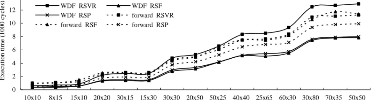
(5) Int. Computer Symposium, Dec. 15-17, 2004, Taipei, Taiwan.. Table 1. Experimental results (2 multipliers and 2 adders) (length, d). 2 memory modules Wave Digital Filter Forward-substitution IIR 2D Filter Discrete Fourier Transform THCS. 3 memory modules. 4 memory modules. RSVR RSF. RST. RSP RSVR RSF. RST. RSP RSVR RSF. 5,2 6, 3 24, 1 6, 2 14, 1 4, 2. 9, 3 11, 4 40, 1 10, 3 28, 0 8, 0. 9, 1 5, 3 11, 1 4, 8 40, 1 14, 1 10, 1 5, 3 28, 0 10, 1 8, 0 4, 2. 10, 5 11, 8 40, 1 10, 6 28, 1 8, 1. 9, 1 3, 6 11, 2 4, 8 40, 1 11, 1 10, 1 4, 3 28, 1 8, 3 8, 1 2, 4. 9, 1 11, 3 40, 1 10, 5 28, 2 8, 2. 9, 1 11, 5 40, 1 11, 9 28, 4 8, 3. 9, 2 11, 9 40, 2 11, 15 29, 6 8, 5. RST. RSP. 10, 8 12, 12 40, 3 10, 7 28, 1 8, 1. 9, 1 11, 2 40, 1 10, 1 28, 1 8, 1. F10: 2w × ∑ half (i, N ) i =1. application we only sketch the results of RSF or RST. F11: (w + n – mw) × half (E, N). execution time of RSP is similar to others, sometimes. F12: 2w (n − w) wN  × ∑ half (i, N ) i =1. even outperforms them. Thus, like RSVR, RSF, and. D. depending on which result is better. In this figure, the. N −1. RST, RSP is also an effective and efficient algorithm.. F13: 2w × ∑i =1 half (i, N ) F. 5. F14: (2w + B  A w ) × half (G, N). Concluding Remarks In this paper, we have proposed RSP to schedule. F15: (2C + (w – B)  A w ) × half (H, N). nested loops for DSP systems with multiple memory. The execution time of RSP =. modules. It contains a simple variable partitioning. F1 + F2 + F4 + F5 + F9 + F10 + F11. mechanism, and applies unimodular transformation,. if wm + 1 ≤ w + n. unfolding, and rotation scheduling techniques to. F1 + F3 + F6 + F7 + F8 + F12 + F13 + F14 + F15. schedule both ALU and memory operations. We also use an analytic module and DSP applications to. if wm + 1 > w + n 4.2. evaluate RSP. Based on evaluating results, RSP is. Experimental Results Finally, we select some DSP applications to. actually an efficient and effective algorithm compared. compare RSVR, RSF, RST, and RSP. Suppose both. with RSVR, RSF, and RST.. ALU and memory operations take one time unit to execute, Table 1 list our scheduling results.. Reference. Notice that in our three algorithms an iteration. [1] V. K. Madisetti, VLSI Digital Signal Processors:. contains N original iterations, so the actual execution. An Introduction to Rapid Prototyping and. time of an iteration equals to the value in Table. Design Synthesis, Butterworth-Heinemnn, 1995.. divided by N. From these results, lengths obtained by. [2] J. Eyre and J. Bier, “The Evolution of DSP. all algorithms are similar, but RSP can obviously get. Processors”, IEEE Signal Processing Magazine,. smaller d. The reason is that an iteration in RSP is. Vol. 17, Issue 2, pp. 43-51, March 2000.. composed of N independent original iterations, and its. [3] R. Leupers and D. Kotte, “Variable Partitioning. memory operations will be evenly allocated. Hence,. for Dual Memory Bank DSPs”, Proc. of. the schedule generated by list scheduling will be. International Conference on Acoustics, Speech,. already quite compact, which can decrease times. and Signal Processing, Vol. 2, pp. 1121-1124,. applying retiming technique and retiming depth.. May, 2001.. Figure 5 shows the execution time calculated by. [4] Q. Zhuge, B. Xiao, and E. H. -M. Sha, “Variable. above formulas. Except RSVR and RSP, for each. Partitioning and Scheduling of Multiple Memory. 1324.

(6) Int. Computer Symposium, Dec. 15-17, 2004, Taipei, Taiwan.. Execution time (1000 cycles). 14 WDF RSVR WDF RSP forward RSF. 12 10. WDF RSF forward RSVR forward RSP. 8 6 4 2 0 10x10. 8x15. 15x10 20x20 30x15 15x30 30x30 20x50 50x25 40x40 25x65 60x30 30x80 70x35 50x50 Number of iterations. Execution time (1000 cycles). 16 Filter RSVR Filter RSP THCS RST. 14 12 10. Filter RST THCS RSVR THCS RSP. 8 6 4 2 0 10x10. 8x15. 15x10 20x20 30x15 15x30 30x30 20x50 50x25 40x40 25x65 60x30 30x80 70x35 50x50 Number of iterations. Execution time (1000 cycles). 40 IIR2D RSVR IIR2D RSP DFT RST. 35 30 25. IIR2D RSF DFT RSVR DFT RSP. 20 15 10 5 0 10x10. 8x15. 15x10 20x20 30x15 15x30 30x30 20x50 50x25 40x40 25x65 60x30 30x80 70x35 50x50 Number of iterations. Figure 5.. Experimental results (2 multipliers, 2 adders, and 3 memory modules).. Architectures for DSP”, Proc. of International. Synchronous Circuitry”, Algorithmica, Vol. 6, No.. Parallel and Distributed Processing Symposium,. 1, pp. 5-35, June 1991. [8] M. E. Wolf and M. S. Lam, “A Loop Transforma-. pp. 130-136, April 2002. [5] Y. -H. Lee and C. Chen, “Efficient Variable. tion Theory and an Algorithm to Maximize Para-. Partitioning and Scheduling Methods of Multiple. llelism”, IEEE Trans. on Parallel and Distributed. Memory Modules for DSP”, Proc. of 10. th. Systems, Vol. 2, No. 4, pp. 452-471, Oct. 1991.. Workshop on Compiler Techniques for High-. [9] Y. -H. Lee and C. Chen, “A Two-level. performance Computing, pp. 80-89, March 2004.. Scheduling Method: An Effective Parallelizing. [6] L. Lamport, “The Parallel Execution of DO. Technique for Uniform Nested Loops on a DSP. Loops”, Comm. ACM SIGPLAN, Vol. 17, No. 2,. Multiprocessor”, accept and to appear to Journal. pp. 82-93, Feb. 1974.. of Systems and Software.. [7] C. E. Leiserson and J. B. Saxe, “Retiming. 1325.

(7)