First-order analysis of a two-conjugate zoom system

First-order analysis of a two-conjugate

zoom system

Mau-Shiun Yeh

National Chiao Tung University Institute of Electro-Optical Engineering 1001 Ta Hsueh Road

Hsin Chu 30050, Taiwan

Shin-Gwo Shiue

Industrial Technology Research Institute Opto-Electronics & Systems Laboratories Q000 OES/ITRI

Building 44, 195-8 Chung Hsing Road, Section 4

Chutung, Hsin Chu, 310, Taiwan

Mao-Hong Lu,MEMBER SPIE National Chiao Tung University Institute of Electro-Optical Engineering 1001 Ta Hsueh Road

Hsin Chu 30050, Taiwan E-mail: mhlu@jenny.nctu.edu.tw

Abstract. A general analysis for the first-order design of the

two-conjugate zoom system, which consists of three lenses and has a real or virtual image, is presented. The design formulas are derived. Of two-conjugate zoom systems, we analyze the solution areas in the system parameter diagrams under two particular initial conditions in which the object/image and pupil magnifications of the middle lens are taken to be 1 and 21 or 21 and 1. Two design methods are proposed. Several examples are given to demonstrate the proposed design procedures. © 1996 Society of Photo-Optical Instrumentation Engineers.

Subject terms: two-conjugate zoom lenses.

Paper 08026 received Feb. 13, 1996; revised manuscript received May 18, 1996; accepted for publication May 20, 1996.

1 Introduction

A zoom system is generally considered to consist of three parts: the focusing, zooming, and fixed parts. The focusing part is placed in front of the zooming part, to adjust the object distance. The zooming part is literally used for zooming and the fixed rear part serves to control the focal length or magnification and reduce the aberrations of the whole system. Some published papers1 concentrate on the first-order zoom design in which only the object/image dis-tance is fixed. However, few of them discuss the possible solutions in the first-order design. Oskotsky2 describes a graphoanalytical method for the first-order design of two-lens zoom systems and discusses the region of Gaussian solution. Johnson and Feng3use a methodology to discuss the potential solutions for a mechanically compensated zoom lenses with a single moving element. We have also proposed a two-optical-component method for designing zoom system.4

In a general zoom system, the aperture stop is usually placed after the moving elements and before a fixed lens, so the exit pupil position is fixed but the entrance pupil posi-tion varies widely in zooming. In some optical systems, the wandering of the entrance pupil is not a great disadvantage. However, the variation of the entrance pupil position could be a very serious disadvantage for a large-zoom-ratio sys-tem or a zoom-phase-contrast microscope.

A two-conjugate zoom system is the one in which not only the object and image but also the entrance and exit pupils are fixed during zooming. Such a zoom system re-quires at least three lenses that move separately. Hopkins5 proposed the first-order design formulas for a special sym-metrical two-conjugate zoom system. In that case, the pow-ers of the first and third lenses are the same and the middle lens has a power with an opposite sign; the distance from

object to entrance pupil and the distance from image to exit pupil are equal, but in opposite direction; the object/image and pupil magnifications are numerically reciprocal and in opposite sign; and the power of the system is the same for any given magnification and its reciprocal. In the mean position of zooming, he assumes the system has object/ image magnification M521 and pupil magnification

M¯ 51, and the magnification of the middle lens M2 is21. Following the method described by Hopkins, Shiue6 dis-cussed the two-conjugate zoom system with M51, M¯

521, and M251 in the mean position of zooming. In this paper, we analyze a general two-conjugate zoom system that consists of three lenses and has a real or virtual image. The powers of the three lenses and the positions of object, image, entrance, and exit pupils are not constrained as those in the symmetrical system proposed by Hopkins.5 To simplify the design, we discuss two special two-conjugate zoom systems in which the object/image and pu-pil magnifications of the middle lens at the initial condition are 1 and 2 1 or 21 and 1. In both cases, we find the possible solutions for the positions of object, image, en-trance, and exit pupils, which are related to the power val-ues of the three lenses, with the graphoanalytical method.2 Two design methods are discussed. Four examples are pre-sented to demonstrate this analysis.

2 Theory

2.1 General Design Formulas

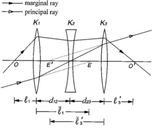
The notation used in this paper is shown in Fig. 1. The object O is imaged at O

8

with a object/image magnification

M and the entrance pupil E is imaged at the exit pupil E

8

with a pupil magnification M¯ . Here

l

and

l

8

are the dis-tances from the first principal plane to the object and the

second principal plane to the image, respectively. Similarly,

l

¯ and

l

¯

8

are the distances from the first principal plane to the entrance pupil and the second principal plane to the exit pupil. In this paper, the distance to the right of the reference point is positive; that to the left is negative. In this analysis, we take the paraxial and thin-lens approximations. For a thin lens, both the principal planes coincide with the lens. The general conjugate equation gives

M L

8

2 1 M L5K5 1 F, ~1!

where K and F are the equivalent power and focal length of the system, respectively; L5(OE) is the distance from ob-ject to entrance pupil of the system; and L

8

5(O

8

E

8

) is the distance from image to exit pupil of the system. From Gaussian optics, we have

L5

l

¯2

l

5

S

1 M¯ 2

1

M

D

F, ~2!

L

8

5

l

¯

8

2

l

8

5~M2M¯ !F. ~3!

With the distance from the first to the second principal plane,D5~HH

8

!, we have

KD5PK2

S

22M21

M

D

, ~4!

where P is the distance from object to image~OO

8

!. For a three-lens system with powers K₁, K₂, and K₃and interlens separations d12and d23, the power K and the dis-tanceD are given by

K5K11K21K32dK1K32~d12K11d23K3!K2 1d12d23K1K2K3, ~5! KD52d2K1K32~d12 2 K11d23 2 K3!K21dd12d23K1K2K3, ~6!

where d5d121d23. Here, d12can be expressed as

d125

l

1

8

2

l

25~12M1!F12

S

1 M2 21

D

F2, ~7! or d125

l

¯1

8

2

l

¯25~12M¯1!F12

S

1 M¯2 21

D

F2, ~8!

where M1( M¯1) and M2( M¯2) are the object/image~pupil! magnifications of the first and second lenses, respectively. Using Eqs.~7! and ~8!, we have

F252

M₁2M¯₁

1/M221/M¯2

F1. ~9!

Similarly, d23 can be expressed as

d₂₃5

l

2

8

2

l

35~12M2!F22

S

1 M3 21

D

F₃, ~10! or d235

l

¯2

8

2

l

¯35~12M¯2!F22

S

1 M¯3 21

D

F3. ~11!

From Eqs.~10! and ~11!, we have

F352

M22M¯2 1/M321/M¯3

F2. ~12!

Note that L and L

8

can also be regarded as the distances from object to entrance pupil of the first lens and from image to exit pupil of the third lens, respectively. So we have L5

l

¯12

l

15

S

1 M¯1 2 1 M1

D

F1 ~13! and L

8

5

l

¯3

8

2

l

8

35~M32M¯3!F3. ~14! From Eqs. ~1! to ~6! with different values of K₁, K₂, and

K3, we can obtain a zoom system. However, it is difficult to get a satisfactory result by generally solving the preced-ing equations. To get a desirable solution easily, some con-straints in solving are needed.

2.2 Two Special Initial Conditions

As mentioned, the special initial conditions in which the object/image magnification M2and pupil magnification M¯2 of the middle lens are 1 and21 or 21 and 1 in the initial position are assumed. In the following, we discuss the so-lutions under these two initial conditions.

2.2.1 Case 1: M₂51 and M¯₂521

In this case, the marginal ray is through the center of the middle lens, as shown in Fig. 2. Substituting M₂51 and

M¯2521 into Eqs. ~9! and ~12!, we have

Fig. 1 Diagram of the Gaussian optics:PandP¯ are the distance from object to image and the distance from entrance to exit pupil, respectively.

F252 M12M¯1 2 F1, ~15! F352 2 1/M321/M¯3 F2. ~16!

In paraxial approximation, we have

l

15

S

1 M1 21

D

F1, ~17!

l

¯15

S

1 M¯1 21

D

F1, ~18!

l

3

8

5~12M3!F3 ~19!

l

¯3

8

5~12M¯3!F3. ~20!

Equations~17! to ~20! indicate the positions of object, en-trance pupil, image, and exit pupil. From these equations, we find that the positions of two pairs of conjugate planes are related to the values of F1, F2, and F3, and the values of object/image and pupil magnifications of each lens.

Substituting the initial condition, M251 and M¯2521, into Eqs. ~7!, ~8!, ~10!, and ~11! and using Eqs. ~18! and

~20!, we get d125~12M1!F1, ~21! d125~12M¯1!F112F2, ~22! d1252 F₁2

l

¯11F1 1~F112F2!, ~23! d2352

S

1 M₃21

D

F3, ~24! d2352F22

S

1 M¯3 21

D

F3, ~25! d235 F₃2

l

¯3

8

2F3 1~F312F2!. ~26!

The interlens separations d₁₂ and d₂₃ must be positive in zooming. This provides some constraints on the solution, i.e., on

l

1,

l

¯1,

l

8

3, and

l

¯3

8

. Under these constraints, we can calculate the solution ranges of

l

1 and

l

3

8

with Eqs.

~17!, ~19!, ~21!, and ~24!. From Eq. ~23!, we can also find

the solution ranges of

l

¯1 for different combinations of F1 and F2. Similarly, from Eq. ~26! we obtain the solution ranges of

l

¯3

8

for different combinations of F2and F3. All the results for

l

1and

l

¯1are shown in Tables 1 and 2 and for

l

3

8

and

l

¯3

8

in Tables 3 and 4.

By using Eqs. ~15!, ~18!, and ~21!, F₁2/(F₁12F₂) in Table 2 becomes

Fig. 2 Three-lens zoom system with the initial conditionsM251 and

M¯₂₅₂1. The marginal ray is through the center of the middle lens.

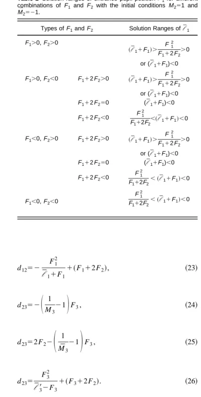
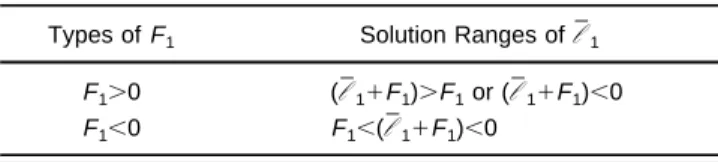
Table 1 Solution ranges of object positionl 1for different types of

F1with the initial conditionsM251 andM¯2521. Types ofF₁ Solution Ranges ofl1

F1.0 (l11F1).F1or (l 11F1),0

F1,0 F1,(l 11F1),0

Table 2 Solution ranges of entrance pupil positionl¯1for different combinations of F₁ and F₂ with the initial conditions M₂₅1 and

M¯2521.

Types ofF₁andF₂ Solution Ranges ofl¯1

F1.0,F2.0 ~l¯11F1!. F₁2 F112F2. 0 or (l¯11F1),0 F₁.0,F₂,0 F₁12F₂.0 _~l¯ 11F1!. F₁2 F₁₁2F₂.0 or (l¯11F1),0 F112F250 (l¯11F1),0 F112F2,0 F₁2 F112F2,~ l¯11F1!,0 F_1,0,F_2.0 F₁₁2F_2.0 _~l¯ 11F1!. F₁2 F112F2. 0 or (l¯11F1),0 F₁12F₂50 (l¯11F1),0 F112F2,0 F₁2 F₁₁2F₂, ~l¯11F1!,0 F_1,0,F_2,0 F₁2 F112F2, ~ l¯11F1!,0

F₁2 F112F2 5

l

¯11F1 11@~12M1!F1/F1 2_#~

l

¯11F1! 5 ~

l

¯11F1! 11~d12/F1 2_!~

l

¯11F1! . ~27!

Here d₁₂must be positive. The value of 11d₁₂~

l

¯11F1!/F1 2 is greater than 1 if

l

¯11F1.0 and is between 0 and 1 if

l

¯11F1,0 and F112F2,0, so the inequality equation

l

¯11F1.F12/(F112F2) in Table 2 is always true. It means that the constraints

l

¯11F1.F1

2_/(F

112F2).0 and

F12/(F112F2),

l

¯11F1,0 are actually equivalent to the conditions

l

¯11F1.0 and

l

¯11F1,0, respectively.

By using Eqs. ~16!, ~20!, and ~24!, the term

2F3 2_/(F 312F2) in Table 4 becomes 2F 3 2 F₃12F₂5 ~

l

¯3

8

2F3! 12@2~1/M₃21!F₃/F ₃2#~

l

¯3

8

2F3! 5 ~

l

¯ 3

8

2F3! 12~d₂₃/F ₃2!~

l

¯3

8

2F3! . ~28!

Here d23 must be positive. The value of 1 2 d23(

l

¯3

8

2 F3)/F 3 2

is greater than 1 if

l

¯3

8

2 F3, 0 and is between 0 and 1 if

l

¯3

8

2 F3 . 0 and F312F2,0, so the inequality equation2 F ₃2/(F31 2F2).

l

¯3

8

2 F3in Table 4 is always true. It means that the constraints

l

¯3

8

2 F3 , 2F 3

2 /(F3

1 2F2), 0 and2 F3 2

/(F31 2F2).

l

¯3

8

2 F3. 0 areactu-ally equivalent to the conditions

l

¯3

8

2 F3, 0 and

l

¯3

8

2 F3

. 0, respectively.

By using Eqs.~15!, ~17!, and ~18!, the term F₁12F₂in Table 2 can also be written as

F₁12F₂5F₁2~

l

¯

11F1!2~

l

11F1!

~

l

¯11F1!~

l

11F1!

F ₁2. ~29!

The curve for F112F250 is a hyperbola in the

l

1;

l

¯1 diagram. The solution distribution in the diagram is thus divided into several areas by the hyperbolic curves and the sign of F₁12F₂.

By using Eqs.~16!, ~19!, and ~20!, F312F2 in Table 4 can be expressed as

F312F25F31

~

l

¯3

8

2F3!2~

l

3

8

2F3!

~

l

¯3

8

2F3!~

l

3

8

2F3!

F ₃2. ~30!

Thus, F312F250 gives another hyperbola in the

l

3

8

;

l

¯3

8

diagram. Similarly, in this diagram, the solution distribu-tion is thus divided into several areas by the hyperbolic curves and the sign of F₃12F₂.

According to the different values of F1, F2, and F3, we can illustrate the solution areas in the

l

1 ;

l

¯1 and

l

3

8

;

l

¯3

8

diagrams, as shown in Figs. 3 and 4, where we make coordinate transforms from

l

1~

l

¯1! to

l

11F1~

l

¯11F1! in the object~entrance pupil! space of the first lens and from

l

3

8

(

l

¯3

8

) to

l

8

32 F3(

l

¯3

8

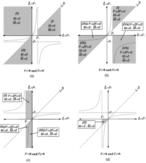
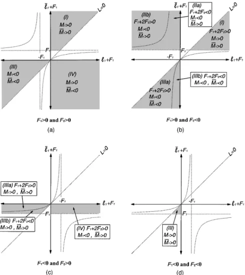
2 F3) in the image~exit pupil! space of the third lens to make the magnifications have the same sign in each quadrant.

Figure 3 shows the solution areas of the object distance and entrance pupil distance of the first lens for different combinations of F₁and F₂. Each solution area gives some constraints on the signs of the related parameters including

F₁12F₂, M₁, and M¯₁. From Eq. ~15!, the sign of ( M12M¯1) in each area is determined by the sign of F2, which is given when the solution area is chosen. The sign of L5~

l

¯12

l

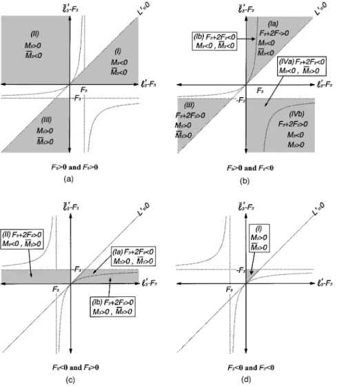
1!, which is the distance from object to the entrance pupil, is positive in the upper-left section and negative in the lower-right section.

Similarly, Fig. 4 shows the solution areas of the image distance and exit pupil distance of the third lens for differ-ent combinations of F2and F3. This figure shows the con-straints on the signs of the related parameters, including

F312F2, M3, and M¯3, in each solution area. Similar to L, the sign of L

8

5 (

l

¯3

8

2

l

3

8

), which is the distance from

im-Table 3 Solution ranges of image positionl 38for different types of

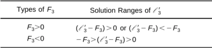
F₃with the initial conditionsM₂51 andM¯₂521. Types ofF₃ Solution Ranges ofl38

F3.0 (l 382F3).0 or (l 382F3), 2F3

F_3,0 ₂F3.(l 382F3).0

Table 4 Solution ranges of exit pupil positionl¯38for different com-binations ofF₂andF₃with the initial conditionsM₂₅1 andM¯₂₅₂1. Types ofF2andF3 Solution Ranges ofl¯38

F_3.0,F_2.0 _~l¯ 3 82F3!.0 or ~l¯382F3!, 2F₃2 F₃₁2F₂,0 F_3.0,F_2,0 F₃₁2F_2.0 ~l¯382F3!.0 or ~l¯382F3!, 2F₃2 F312F2, 0 F₃₁2F₂₅0 _~l¯ 3 82F3!.0 F312F2,0 2 F₃2 F312F2.~ l¯382F3!.0 F_3,0,F_2.0 F₃₁2F_2.0 _~l¯382F3!.0 or ~l¯382F3!, 2F₃2 F312F2, 0 F312F250 ~l¯382F3!.0 F312F2,0 2F₃2 F312F2.~ l¯382F3!.0 F₃,0,F₂,0 2F32 F312F2.~ l¯382F3!.0

age to the exit pupil, is positive in the upper-left section and negative in the lower-right section.

In Figs. 3 and 4, on the boundaries of solution areas the solutions of interlens separation may be zero or infinite and are not discussed here. If the solution points are on the hyperbolic curves in Figs. 3 or 4, we would have the results of F₁12F₂50 or F₃12F₂50.

2.2.2 Case 2: M₂521 and M¯₂51

In this case, the principal ray is through the center of the middle lens as shown in Fig. 5, Substituting M₂521 and

M¯251 into Eqs. ~7! to ~12!, we get

F₂5M12M ¯ 1 2 F1, ~31! F35 2 1/M321/M¯3 F2, ~32! d₁₂5~12M₁!F₁12F₂ ~33! d1252 F 1 2

l

11F11~F112F2!, ~34! d₁₂5~12M¯₁!F₁, ~35! d2352F22

S

1 M3 21

D

F3, ~36! d235 F 3 2

l

3

8

2F31~F 312F2!, ~37! d2352

S

1 M¯3 21

D

F3. ~38!

We also have the same equations as Eqs.~17! to ~20!,

l

15

S

1

M₁21

D

F1 ~39!

Fig. 3 Solution areas in thel1;l¯1diagram are indicated with shadow regions: (a) to (d) show the solution areas for different combinations ofF1andF2with the initial conditionsM251 andM¯2521. The constraints on the signs ofF₁₁2F₂,M₁, andM¯₁in each area are also shown. The value ofLis positive at the upper-left section and negative at the lower-right section. The hyperbola represents the curves ofF₁₁2F₂₅0.

l

¯15

S

1 M¯1 21

D

F1, ~40!

l

3

8

5~12M3!F3, ~41!

l

¯3

8

5~12M¯3!F3. ~42!

In the same way as we did in case 1, we get the solution ranges for

l

1,

l

¯1,

l

3

8

, and

l

¯3

8

, as listed in Tables 5 through 8. According to the different values of F₁, F₂, and

F3, the solution areas in the

l

1;

l

¯1and

l

3

8

;

l

¯3

8

diagrams are shown in Figs. 6 and 7.

Fig. 4 Solution areas in thel38;l¯38diagram are indicated with shadow regions: (a) to (d) show the solution areas for different combinations ofF2andF3with the initial conditionsM251 andM¯2521. The constraints on the signs ofF₃12F₂,M₃, andM¯₃in each area are also shown. The value ofL8is positive at the upper-left section and negative at the lower-right section. The hyperbola represents the curves ofF312F250.

Fig. 5 Three-lens zoom system with the initial conditionsM₂₅₂1 andM¯251. The principal ray is through the center of the middle lens.

2.3 Interlens Separations d₁₂and d₂₃in Zooming To find the positions of the three lenses for a given magni-fication M during zooming, we must calculate d12and d23. From Eqs.~5! and ~6! we have

d12d235

KD2~K2K12K22K3!d

K₂~K₁1K₃! . ~43!

Substituting d₁₂d₂₃into Eq.~5!, we have the relation of the interlens separations d12 and d23 as follows:

d235Ad121B, ~44! where A52K1~K1K21KK3! K3~K2K31KK1! , ~45! and B5

S

K₁1K₂1K₃2K1 K1K3 K11K3 KD

D

K11K3 K3~K2K31KK1! . ~46!

Using Eqs.~5! and ~44!, we find

d125 2b6~b2_24ac!1/2 2a , ~47! where a5AK1K2K3, b5BK1K2K32AK3~K11K2!2K1~K21K3!, c5K11K21K32K2BK3~K11K2!.

We substitute the given values of L, L

8

, and P, which are from the initial position, into Eqs. ~1! and ~4! to get the values of K and KD as the functions of M. Then we can obtain the interlens separations with Eqs.~44! and ~47! for each M value. After solving for d12 and d23, we calculate the distance

l

1 from the first lens to the object and the

Table 5 Solution ranges of entrance pupil positionl¯1for different types ofF₁with the initial conditionsM₂₅₂1 andM¯₂₅1.

Types ofF1 Solution Ranges ofl¯1

F₁.0 (l¯11F1).F1or (l¯11F1),0

F1,0 F1,(l¯11F1),0

Table 6 Solution ranges of object positionl 1for different combina-tions ofF₁andF₂with the initial conditionsM₂₅₂1 andM¯₂₅1.

Types ofF1andF2 Solution Ranges ofl 1

F1.0,F2.0 ~l 11F1!. F ₁2 F₁₁2F₂.0 or (l 11F1),0 F1.0,F2,0 F112F2.0 ~l 11F1!. F ₁2 F112F2. 0 or (l 11F1),0 F₁₁2F₂₅0 (l 11F1),0 F₁₁2F_2,0 F1 2 F₁₁2F₂,~l 11F1!,0 F1,0,F2.0 F112F2.0 ~l 11F1!. F ₁2 F₁₁2F₂.0 or (l 11F1),0 F112F250 (l 11F1),0 F₁₁2F_2,0 F1 2 F112F2,~ l 11F1!,0 F_1,0,F_2,0 _F 1 2 F₁₁2F₂,~l 11F1!,0

Table 7 Solution ranges of exit pupil positionl¯38 for different types ofF₃with the initial conditionsM₂₅₂1 andM¯₂₅1.

Types ofF3 Solution Ranges ofl¯38

F_3.0 _(l¯ 3

82F₃)_.0 or(l¯382F3), 2F3

F₃,0 _2F

3.(l¯382F3).0

Table 8 Solution ranges of image positionl38for different combina-tions ofF2andF3with the initial conditionsM2521 andM¯251.

Types ofF2andF3 Solution Ranges ofl 38

F_3.0,F_2.0 _~l 3 82F3!.0 or ~l 382F3!, 2F₃2 F₃₁2F₂,0 F3.0,F2,0 F312F2.0 ~l 382F3!.0 or ~l 382F3!, 2F₃2 F312F2, 0 F₃12F₂50 (l 382F3).0 F312F2,0 2F₃2 F312F2.~ l382F3!.0 F_3,0,F_2.0 F₃₁2F_2.0 _~l 3 82F3!.0 or ~l 382F3!, 2F₃2 F₃₁2F₂,0 F312F250 ~l 382F3!.0 F312F2,0 2 F₃2 F₃₁2F₂.~l 382F3!.0 F_3,0,F_2,0 2F₃2 F312F2.~ l382F3!.0

distance

l

3

8

from the last lens to the image in any zooming position. In doing so, we need the values ofd~the distance from the first moving lens to the first principal plane H! and d

8

~the distance from the last moving lens to the second

principal plane H

8

!, as shown in Fig. 1. These quantities can be calculated using

d5d23K31d12~K21K32d23K2K3!

K , ~48!

d

8

52d12K11d23~K1_K1K22d12K1K2!. ~49!

So

l

1and

l

3

8

are given by

l

15

l

1d, ~50!

l

3

8

5

l

8

1d

8

, ~51!

where

l

5(1/M21)F and

l

8

5(12M)F.

3 Design Methods

To simplify the solving of a two-conjugate zoom system, we could give some related parameters in the initial posi-tion of zooming. If one of the two special initial condiposi-tions is selected as mentioned in Sec. 2.2, M2 and M¯2 will be determined. Besides, it can be seen from Eqs. ~15! to ~26! or Eqs.~31! to ~42! that we still need the other five param-eters, which could be the focal lengths of the three lenses, the object or entrance pupil distance from the first lens, the image or exit pupil distance from the third lens, the object/ image or pupil magnifications of the first and third lenses, and the distance from object to image, etc. We propose two useful calculating procedures as follows.

3.1 Given

l

1,

l

¯1,

l

3

8

,

l

¯3

8

, and F1

According to the system requirements and the expected signs of powers for the three lenses, we give the positions of the object, entrance pupil, image and exit pupil in the initial position and obtain the values of L and L

8

. One of the solution areas of Figs. 3 or 6 for

l

1 and

l

¯1 can be

Fig. 6 Solution areas in thel1;l¯1diagram are indicated with shadow regions: (a) to (d) show the solution areas for different combinations ofF₁andF₂with the initial conditionsM₂₅₂1 andM¯₂₅1. The constraints on the signs ofF112F2,M1, andM¯1in each area are also shown. The value ofLis positive at the upper-left section and negative at the lower-right section. The hyperbola represents the curves ofF₁₁2F₂₅0.

chosen according to the given values of

l

1and

l

¯1and the expected signs of F1and F2. The initial values of M2and

M¯₂ depend on the selected initial conditions. We then choose a value of F1 according to the constraint in the chosen solution area and calculate M₁ and M¯₁ from Eqs.

~17! and ~18! or Eqs. ~39! and ~40!. The value of F2can be found from Eqs. ~15! or ~31!. With Eqs. ~2! and ~3!, we have

L

8

L 5M M¯ 5M1M2M3M ¯

1M¯2M¯3. ~52! Combining this equation with Eqs. ~19! and ~20! or Eqs.

~41! and ~42!, we have M3as follows:

M35 2b6~b2_24ac!1/2 2a , ~53! where a51, b5

S

l

3

8

l

¯3

8

21

D

, c52

S

l

3

8

l

¯3

8

DS

L

8

L

D

1 M1M2M¯1M¯2 ,

and M¯3is given by Eq.~52!. The value of F3is calculated from Eqs. ~16! or ~32!. The interlens separations d₁₂ and

d23 are found from Eqs.~21! to ~26! or Eqs. ~33! to ~38!. The distance from object to image P is obtained from the following equation:

Fig. 7 Solution areas in thel38;l¯38diagram are indicated with shadow regions: (a) to (d) show the solution areas for different combinations ofF₂andF₃with the initial conditionsM₂521 andM¯₂51. The constraints on the signs ofF312F2,M3, andM¯3in each area are also shown. The value ofL8is positive at the upper-left section and negative at the lower-right section. The hyperbola represents the curves ofF₃₁2F₂₅0.

P5

S

22M12 1 M1

D

F11

S

22M22 1 M2

D

F2 1

S

22M32 1 M₃

D

F3. ~54!

If the initial structure is not satisfactory or the values of

l

3

8

2 F3and

l

¯3

8

2 F3together with F2and F3are not lo-cated in the solution areas of Figs. 4 or 7 for

l

3

8

and

l

¯3

8

, we should adjust the related input parameters or choose another solution area. After obtaining the desirable result and the structure of zoom system under the initial condi-tion, we can calculate the related parameters during zoom-ing.

In zooming, the system magnification M changes; L, L

8

, and P, which we have known from the initial position, remain constant. We can find K and KD with Eqs. ~1! and

~4! for any M value. We then find the interlens separations

d12 and d23 from Eqs. ~44! and ~47!, and the object and image distances

l

1and

l

3

8

from Eqs.~50! and ~51! during zooming. If the loci of the lenses are not smooth or the zoom ratio of the system is too small, of course, we can readjust the related input parameters or select the other ini-tial condition.

3.2 Given L,

l

1(or

l

¯1), P, M, and F1

In practical design, the value of L5~

l

¯12

l

1! is often given from the preceding system and the object/image distance P will also be a given value if the zoom lens is used as a relay system. In this case, if the object ~or entrance pupil! dis-tance from the first lens,

l

1 ~or

l

¯1! is given, we will find

l

¯1~or

l

1! from L5~

l

¯12

l

1!. The system magnification M may also be taken as an input parameter in the initial posi-tion. In this case, the value of M is often taken as 1 or21. According to the given values of

l

1,

l

¯1, P, and M , and the expected signs of powers for the three lenses, we choose one of the solution areas of Figs. 3 or 6 for

l

1 and

l

¯1. Since the initial condition gives the values of M2 and M¯2, we can calculate M1 and M¯1 with Eqs. ~17! and ~18! or Eqs.~39! and ~40! if a value of F₁is given according to the constraint in the chosen solution area. We also find the value of F₂ from Eqs. ~15! or ~31! and obtain the focal length F3of the third lens from the following equations:

F35

F

P2

S

22M12 1 M1

D

F12

S

22M22 1 M2

D

F2

G

Y

S

22M32 1 M3

D

, ~55! and M35 M M₁M₂. ~56!

The M¯3value is calculated with the following formulas:

P2L5P¯2L

8

, ~57! P ¯5

S

22M¯12 1 M¯1

D

F11

S

22M¯22 1 M¯2

D

F2 1

S

22M¯32 1 M¯3

D

F3, ~58!

where P¯ is the distance from entrance to exit pupil ~EE

8

! and we have M¯35 F3 L2P1~22M¯121/M¯1!F11~22M¯221/M¯2!F21~22M3!F3 , ~59!

l

3

8

and

l

¯3

8

are calculated from Eqs. ~19! and ~20! or Eqs.

~41! and ~42!, and L

8

is then found from Eq. ~14!. The interlens separations d12 and d23 are obtained with Eqs.

~21! to ~26! or Eqs. ~33! to ~38!. If the initial structure is not

satisfactory or the values of

l

3

8

2 F3and

l

¯3

8

2 F3together with F2and F3are not located in the solution areas of Figs. 4 or 7 for

l

3

8

and

l

¯3

8

, the related input parameters should be adjusted or another solution area should be chosen. In zooming, we obtain the interlens separations d₁₂ and d₂₃ and the object and image distances

l

1 and

l

3

8

with the procedures described in Sec. 3.1.

4 Examples

Using the method described, we design four different zoom systems. To obtain a zoom ratio R, the zoom system is usually arranged to have the overall magnification varied fromuMu5

A

R touMu5 1/

A

R.

4.1 Example 1: Given

l

1590,

l

¯152130,

l

3

8

5 280, and

l

¯3

8

5125

In this example, the object and image are virtual and the entrance and exit pupils are real in the initial position so that L is negative and L

8

is positive. We can find several possible solution areas in Figs. 3 and 6. If we expect that the zoom system comprises two positive lenses and a nega-tive lens in between and has M251 and M¯2521 as the initial conditions, the solution area marked with (IVb) of Fig. 3~b! for

l

1 and

l

¯1 can be chosen. The calculation follows the procedures described in Sec. 3.1. If we give

F1550, we obtain M150.357143, M¯1520.625,

M₃52.64869, M¯₃521.576079, d₁₂532.143, and

d23530.204 in the initial position. We also get

F₂5224.5536, F₃548.5234, and the results of F₁12F₂.0 and F₃12F₂,0. The values of

l

3

8

2 F3 and

l

¯3

8

2 F3are located in the solution area marked with (IIb) of Fig. 4~b! for

l

3

8

and

l

¯3

8

. During zooming, the result is shown in Fig. 8, with the natural logarithm ofuMu as ordi-nate. The system has a zoom ratio of 16:1, magnification M from 4 to 0.25.

4.2 Example 2: Given

l

152100,

l

¯152320,

l

3

8

590, and

l

¯3

8

5295

In this case, we have different values of

l

1,

l

¯1,

l

3

8

, and

l

¯3

8

but the same L5~

l

¯12

l

1! and L

8

5 (l¯3

8

2 l3

8

), as com-pared with the previous example. Here, the object, image,

entrance, and exit pupils are all real. If the zoom system comprises two positive lenses and a negative lens in be-tween and the initial conditions are chosen to be M₂521 and M¯251, we can select the solution area marked with (IIIa) of Fig. 6~b! for

l

1 and

l

¯1. Following the proce-dures described in Sec. 3.1 and giving F1550, we obtain

M1521, M¯1520.185185, M3520.939344, M¯3

525.356738, d12559.259, and d23555.071 in the initial position. We also have F25220.3704, F3546.4075, and the results of F₁12F₂.0, F₃12F₂.0. The values of

l

3

8

2 F3and

l

¯3

8

2 F3are located in the solution area marked with (Ia) of Fig. 7~b! for

l

3

8

and

l

¯3

8

. During zooming, the result is shown in Fig. 9. The system has a zoom ratio of 16:1. The magnification M is from24 to 20.25.

4.3 Example 3: Given

l

152105,

l

¯1580,

l

3

8

5 105, and

l

¯3

8

5 280

Here the object and image are real and the entrance and exit pupils are virtual in the initial position. From the given data, we have positive L, negative L

8

, and L52L

8

. If the system consists of two positive lenses and a negative lens located in between and the initial conditions give M₂521 and M¯251, the solution area marked with (IIb) of Fig. 6~b! can be chosen. In the same way giving F₁540, we obtain M1520.615385, M¯150.333333, M3521.625,

M¯₃53, d₁₂526.667, and d₂₃526.667 in the initial position.

We also have F25218.9744, F3540, and the values of

l

3

8

2 F3and

l

¯3

8

2 F3located in the solution area marked with (IVb) of Fig. 7~b!. In this example, the system is symmetrical and has F₁5F₃, d₁₂5d₂₃, M₁51/M₃, and

M¯151/M¯3 in the initial position. During zooming, the re-sult is shown in Fig. 10. The system has a zoom ratio of 16:1. The magnification M is from24 to 20.25.

4.4 Example 4: Given L5195,

l

152105 (or

l

¯1590), P5270, and M521

In this case, the object is real and the entrance pupil is virtual in the initial position, so that L is positive. We ex-pect that the system has two positive lenses and a negative lens in between. If we select the initial conditions in which

M2521 and M¯251, we can choose the solution area marked with (IIb) of Fig. 6~b!. Because M is 21, M₁ is equal to 1/M3 in the initial position. Following the calcu-lating procedures described in Sec. 3.2 and giving F₁542, we obtain M1520.666667, M¯150.318182, M3521.5,

M¯₃53.299579,

l

3

8

5 106.636,

l

¯3

8

5 298.088, d12528.636, and d23529.727 in the initial position. We also have

F₂5220.6818, F₃542.6545, and the results of F112F2.0, F312F2.0. The values of

l

3

8

2 F3 and

l

¯3

8

2 F3are located in the solution area marked with (IVb) of Fig. 7~b!. During zooming, the result is shown in Fig. 11. The system has a zoom ratio of 16:1 and the magnification

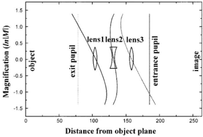
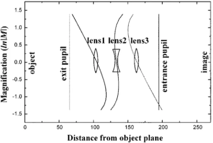
M is from24 to 20.25. Fig. 8 Loci of three lenses in zooming. This system has virtual

ob-ject and image withF₁₅50,F₂₅₂24.5536,F₃₅48.5234, and zoom ratio516. The distance from object to image P is2107.654, the distance from entrance to exit pupilP¯ is 317.347, andL₅₂220 and

L85205.

Fig. 9 Loci of three lenses in zooming. This system has real object

and image withF₁₅50,F₂₅₂20.3704,F₃₅46.4075, and zoom ratio

516, andLandL8are the same as that in Fig. 8. The distance from object to imagePis 304.330, and the distance from entrance to exit pupilP¯ is 729.330.

Fig. 10 Loci of three lenses in zooming. This system is symmetrical

and has real object and image withF1540,F25218.9744,F3540, and zoom ratio₅16. The distance from object to image P is 263.333, the distance from entrance to exit pupilP¯ is2106.667, and

5 Discussion

For the first-order design of two-conjugate zoom lenses, we have analyzed the possible solutions for the positions of two pairs of conjugate planes that correspond to the object/ image and pupils. The solution areas in the

l

1;

l

¯1 and

l

3

8

;

l

¯3

8

diagrams are visual and helpful for designers to select the positive and negative types of three lenses in the zoom system and find the constraints on the powers of lenses if the values of

l

1,

l

¯1,

l

3

8

, and

l

¯3

8

are given in the initial position. In this paper, we give F1and then calculate

F₂ and F₃. Of course, instead of F₁, we can give F₃and then calculate F1 and F2with different design procedures. From Figs. 3 and 4 and 6 and 7, we find that the solution areas for negative first and third lenses are smaller than that for positive first and third lenses. Generally, Eqs.~47! and

~53! should have two solutions. Sometimes only one of

them can meet the conditions d12.0 and d23.0. However, if both the solutions meet these conditions, we will choose the solution that gives a better result.

In examples 1 and 2, two different results are obtained under the same values of L and L

8

but different values of

M₂ and M¯₂, which correspond to the different initial con-ditions described in Sec. 2.2. We also find that the system in example 1 is more compact than that in example 2. In examples 1 to 4, the L and L

8

have opposite signs; this means that the direction from O to E is opposite to that from O

8

to E

8

. However, this is not a necessary condition in our design theory. Systems for different combinations of signs and values of L and L

8

can be solved only if the positions of two pairs of conjugate planes are located in the solution areas shown in the

l

1;

l

¯1and

l

3

8

;

l

¯3

8

diagrams. In many practical designs, we usually expect the initial con-dition is specified in the mean position of zooming, in which the system magnification M is 11 or 21. In this special case, we have one more constraint:uM1u is the re-ciprocal of uM₃u due to M5M₁M₂M₃. The signs of M₁ and M3are the same or not depending on the sign of M2,

11 or 21, such as in example 4. The formulas derived in

this paper are suitable for the general two-conjugate zoom

systems including the symmetrical systems described by Hopkins, who assumed F15F3, L5L

8

,

l

152

l

3

8

, and

l

¯152

l

¯3

8

in the mean position to be the necessary condi-tions. Example 3 is such a case.

6 Conclusion

As we know, a proper first-order layout often gives a sat-isfactory lens design. In general, the layout design of a two-conjugate zoom system is more difficult than that of an ordinary zoom system since both the entrance and exit pu-pils must be fixed during zooming. However, with the analysis of the solution areas in the 2-D diagrams for two pairs of the parameters~

l

1,

l

¯1! and (

l

3

8

,

l

¯3

8

), we can easily find the solutions for the two-conjugate zoom lens.

Acknowledgments

This project was supported by the National Science Council of the Republic of China under the grant No. NSC-85-2215-E-009-004.

References

1. A. Mann and B. J. Thompson, Eds., Selected Papers on Zoom Lenses, SPIE Milestone Series, Vol. MS 85, SPIE Press, Bellingham, WA

~1993!.

2. M. L. Oskotsky, ‘‘Grapho-analytical method for the first-order design of two-component zoom systems,’’ Opt. Eng. 31~5!, 1093–1097

~1992!.

3. R. B. Johnson and C. Feng, ‘‘Mechanically compensated zoom lenses with a single moving element,’’ Appl. Opt. 31~13!, 2274–2278

~1992!.

4. M. S. Yeh, S. G. Shiue, and M. H. Lu, ‘‘Two-optical-component method for designing zoom system,’’ Opt. Eng. 34~6!, 1826–1834

~1995!.

5. H. H. Hopkins, ‘‘2-Conjugate zoom systems,’’ in Optical Instruments and Techniques, pp. 444–452, Oriel Press, Newcastle upon Tyne

~1970!.

6. S. G. Shiue, ‘‘Gaussian optics for 2-conjugate zoom system,’’ Chi-nese J. Opt. Eng. 2~1!, 17–21 ~1985!.

Mau-Shiun Yeh received his BS degree

from the National Taiwan Normal Univer-sity and his MS degree from the National Central University. Currently, he is pursu-ing a PhD at the Institute of Electro-Optical Engineering, National Chiao-Tung Univer-sity. He was an assistant researcher with a major in optical lens design at the Chung Shan Institute of Science and Technology from 1986 to 1993.

Shin-Gwo Shiue received his BS and MS

degrees from the Chung-Cheng Institute of Technology, Taiwan, in 1973 and 1976, and a PhD degree from the University of Reading, United Kingdom, in 1984. He be-came an assistant researcher at the Chung Shan Institute of Science and Technology in 1976. Before receiving his PhD degree, his research interest was mainly solid state laser physics and after-ward concentrated in optical instrument design. He was a president of Taiwan Electro Optical System Com-pany in 1990 and joined the Precision Instrument Developing Center of the National Science Council as a senior researcher in 1994. His current research is optical instrument developing, optical metrology, and lens design.

Fig. 11 Loci of three lenses in zooming. This system has real object

and image withF₁₅42,F₂₅₂20.6818,F₃₅42.6545, and zoom ratio

516. The distance from object to imagePis 270, the distance from entrance to exit pupil P¯ is 2129.724, and L₅195 and

Mao-Hong Lu graduated from the

depart-ment of physics at Fudan University in 1962. He then worked as a research staff member at the Shanghai Institute of Phys-ics and Technology, Chinese Academy of Sciences, from 1962 to 1970 and at the Shanghai Institute of Laser Technology from 1970 to 1980. He studied at the Uni-versity of Arizona as a visiting scholar from 1980 to 1982. He is currently a professor at the Institute of Electro-Optical Engineer-ing, National Chiao-Tung University.