Maximum A Posteriori Restoration of Blurred Image Using Self-Organization

Maximum a posteriori restoration of blurred

images using self-organization

Cheng-Yuan Liou Wen-Pin Tai National Taiwan University

Department of Computer Science and Information Engineering Taipei 10764, Taiwan

E-mail: cyliou@csie.ntu.edu.tw

Abstract. We use the ‘‘magic TV’’ network with the maximum a posteriori (MAP) criterion to restore a space-dependent blurred im-age. This network provides a unique topological invariance mecha-nism that facilitates the identification of such space-dependent blur. Instead of using parametric modeling of the underlying blurred im-age, we use this mechanism to accomplish the restoration. The res-toration is reached by a self-organizing evolution in the network, where the weight matrices are adapted to approximate the blur func-tions. The MAP criterion is used to indicate the goodness of the approximation and to direct the evolution of the network. © 1998 SPIE and IS&T. [S1017-9909(98)01001-0]

1 Introduction

Restoration of a blurred image can be solved by removing the blurs, which are usually caused by an out-of-focus cam-era, linear motion, and the atmospheric turbulence, from the observed image. Blur identification methods have been developed to estimate the unknown blur function in the blurring model, where it is defined as the convolution of an original image with a point spread function~PSF! plus an observation noise. Some methods have focused on simple blurs.1,2Many restoration methods based on the parametric techniques model the original image as a 2-D autoregres-sive moving average~ARMA! process and impose certain statistical assumptions on the image.3Such methods formu-lated the blur identification problem into the parameter es-timation problem. The results are widely diverse according to those assumptions made about the model and the image. Nonparametric methods4–6that employ certain criteria and solve the restoration problem under basic constraints on the PSF have achieved different results.

Several potential methods7,8employ the entropy-related criteria to solve the blur identification problem. In Ref. 7, the unknown blur function is considered as a probability density function and is solved under its a priori knowledge. Since the PSF serves as a density function, the constraints are made to the PSF, for example, nonnegativity, finite sup-port, and energy preserving. The solution must obey these constraints. In Ref. 8, the probability density of the PSF is

also taken into account for blur identification. Maximizing entropy subject to these constraints gives a solution where the PSF tends to satisfy a priori given properties.

We study space-dependent blur functions that also obey the preceding basic constraints. We use a self-organizing network9 following the idea of the ‘‘magic TV’’ and use the maximum a posteriori ~MAP! criterion to evolve the network toward the solution. The ‘‘magic TV’’ provides a natural mechanism to utilize the invariant hidden topology in the image data. All blurs~candidates! that meet this in-variant topology are learned in the network. This criterion guides the network toward the solution.

In the following two sections, we briefly review the im-age and the blur model. The self-organizing network and the MAP criterion are also introduced. Following the crite-rion, we derive the training rule for the network to reach the unknown blur functions. Applications of the network are presented in Sec. 4. The SNR improvement will be used to measure the restoration performance. Based on this mea-sure, we make comparisons between the proposed approach and other methods, including inverse filters, Wiener filters, constrained least squares, Kalman filters, and constrained adaptive restoration.

2 Network and the MAP Criterion

We devise a self-organizing network to learn the blur func-tions. The self-organizing network contains N 5N3N neurons arranged in a 2-D plane. Each neuron i, iPN , has its own weight matrixWi, WiPMm3m. Each weight

ma-trix corresponds to a possible solution for an unknown blur matrix. For blurred image xs,xsPX ,X ,Rm, the

corre-sponding estimated image data yˆs,yˆsPY,Y,Rm, will be

restored by the best-matching weight matrix Wc,cPN ,

using

yˆs5Wc21xs. ~1!

The components in the vector xs are composed of the data

in the m13m2 image matrix Xs, m1•m25m, from one

rectangular region of the blurred image, i.e., x_s[vec(Xs) in lexicographically ordered form,

10_{where the}

vec(Xs) transforms the matrixXs into a vector by stacking Paper CIP-10 received Feb. 10, 1997; revised manuscript received July 1, 1997;

accepted for publication Aug. 1, 1997. 1017-9909/98/$10.00 © 1998 SPIE and IS&T.

the columns of Xs one underneath the other. Solving the

unknown blur matrixWcin Eq.~1! is an inverse problem of

the observation process

xs5Fsys1bs, ~2!

where ys is the original image data, Fs is the real

space-dependent blur matrix, and bs is the noise vector. In Eq.

~2!, each row ofFscorresponds to a PSF. The data xsmay

be contaminated by both the blur and the noise. We attempt to solve a yˆs, which is close to ys, yˆs.ys, from Eq. ~1!.

The object is to solve the best-matching matrixWcand

to derive the original undegraded image data ys from the

observed xs. The difficulty with it is lack of knowledge

about both the unknown blur matrix and the original image data.1 Additional constraints are needed in recovering the image. The basic constraints on the PSF can be accom-plished easily by limiting and normalizing each Wi

prop-erly. The probability densities for all the possible candi-dates Wi, iPN , can be estimated by counting the

excitation frequencies for all neurons. With these densities and the noise model of Eq. ~2!, we can construct an MAP criterion.

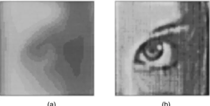
The network is inspired by the ‘‘magic TV.’’9 It pro-vides a platform and mechanism for exploring the hidden topology under severe transformation. The topological in-variance between the input image and the mapped image is the major feature of this mechanism. We utilize this invari-ance to assist the restoration. This network is devised as a self-organized mapping system, which could identify blur features from the input, i.e., the blurred image data. Ac-cording to the ‘‘magic TV,’’ a point source that is ran-domly excited in the input image plane will project a blur feature on the output image plane when the blur aperture is in between the input and the output plane. The implicit topology order of these random point sources can be aligned in a 2-D plane according to their coordinates. The excitations of the corresponding features can also be aligned in a similar topology on the network plane through a self-organizing scheme~see Fig. 1!. The noisy parts of the blur functions do not have such hidden topology. They will be screened out by the ‘‘magic TV’’ mechanism. Thus, we can regularly array these neurons on a rectangular plane with their weight matrices representing~responding to! the blur features.

To achieve statistic average, we use the MAP criterion as the distance measure instead of the linear distance used in the formal self-organization.9The MAP criterion is used to select the best-matching neuron c and to derive the learn-ing rule accordlearn-ingly to evolve the weights toward the un-known blur functions. Given a blurred image data xs, we

plan to determine a Wc that maximizes the a posteriori

probability. The best-matching neuron c among all neurons is determined by

c5arg max

iPN

$p~Wiuxs!%. ~3!

According to the Bayesian analysis, the a posteriori probability ofWigiven xs, p(Wiuxs), can be written in the

form

p~Wiuxs!5

p~Wi!p~xsuWi!

p~xs! }p~

Wi!p~xsuWi!. ~4!

To use this criterion, both the conditional probability p(xsuWi) and the a priori probability p(Wi) should be

ob-tained in advance. The probability p(xs) is assumed to be a

known constant and is omitted from our approach. To determine the a priori probability p(Wi), we count

the excitations~number of times of best-matching! for each neuron i, when a batch of input$xs%are fed to the network.

These excitations are accumulated for each neuron. We then normalize these excitation frequencies. The normal-ized frequency Rˆiis then used as an estimated p(Wi).

Assume the noise in Eq. ~2! is white, zero-mean, and with variances_n2. With a yˆsestimated by Eq. ~1!, the

con-ditional probability p(xsuWi) in Eq.~4! can be formulated

as p~xsuWi!}exp@2E~Wi!#, ~5! where E~Wi!5~xs2Wiyˆs!tD~xs2Wiyˆs!, ~6! and D5diag~1/sn 2_,1/s n 2_,...,1/s n 2_{!. ~7!}

3 Synapse Adaptation in the Network

With the MAP criterion, we derive the adaptation rules for the weight matrices in a generalized self-organization sense.12First, we determine the best-matching neuron c for each blurred input data xs using the formula

Fig. 1 (a) The concept of the ‘‘magic TV’’ for image restoration and (b) the weight matrices in the self-organizing network.

c5arg max i $ p~Wiuxs!% 5arg max i $ p~xsuWi!p~Wi!% 5arg max i $exp@2E~Wi!#Rˆi% 5arg min i $E~Wi!2log~Rˆi!%. ~8!

The best-matching neuron c, which has the minimum value of E(Wi)2log(Rˆi), will be further used. We then substitute

thisWcin Eq.~1! to estimate a temporary value for yˆs.

Then we tune the weight matrices to approach the pos-sible blur matrices. The synapse adaptation rules are de-rived by reducing E(Wc)2log(Rˆc) in Eq. ~8! with respect

to the tuning ofWc. We apply the steep descent method to

updateWc. The weight matrices are adapted by

W_cnew5Wc1akcD•~xs2Wcyˆs!yˆs t

5Wc1a

8

t_{, ~9!}

for the best-matching neuron c, where a and a

8

adapta-tion, and by Wi new₅ Wi1a

8

8

8

for all iPH(c), iÞc, where H~c! is the effective region of the neighborhood function hci in the self-organization.

Since the diagonal component ofDis an unknown constant in Eqs.~9! and ~11!,aDcan be set to a new adaptation rate

a

8

The value of k in Eq.~9! can be intuitively set to kc[ 1 sx_s 2 , ~12! wheres_x s 2

is the variance of the data xs. This means that

we update Eq.~9! safely in a smooth region and carefully in a rough region. Experiments show that this is a good as-signment.

The value kiis introduced to scale the adaptation ofWi

in Eq.~11!. If the distance between neuron i and neuron c is large, the weight matrixWicould not be a candidate of the

current blur function. The scaling of the weight update is needed for accurate mapping. We can set the neighborhood function hcito keep the relationship between kcand kiand

use it in the adaptation rule of Eq.~11! for Wi, iÞc. This

neighborhood function is assigned to a general lateral inter-action function in formal self-organization. Furthermore, this adaptation rule has less computation load than that of the rule in Eq.~10!.

After the adaptation by Eqs. ~9! and ~11!, the weight matrices are modified to satisfy the basic constraints on the

PSF. By the self-organizing learning, various blur functions in the rows are obtained for the space-dependent identifica-tion.

In summary, there are six steps in one training iteration: 1. Find the best-matching neuron c by Eq. ~8! for a

given input data x_s.

2. Estimate the restored image data yˆs from Wcand xs

by Eq.~1!.

3. Tune the values of the training parametersaand h. 4. Adjust the weight matrixWcby Eq. ~9!.

5. Adjust the weight matrices Wi, iPH(c), iÞc, by

Eq.~11!.

6. Modify the weight matrices with respect to the basic constraints on the PSF, nonnegativity and energy pre-serving.

Figure 2 shows a flow chart in an iteration. 4 Simulation Results

We now apply this approach to restore the blurred real images in presence or absence of noise. The simulations are carried out for a scanned 64364 8-bit monochrome image. The original image in absence of noise is shown in Fig. 3. The image in Fig. 3 are sampled from the picture of ‘‘Lena.’’ An image degraded by additive white Gaussian noise with 20-dB signal-to-noise ratio ~SNR! is shown in Figure 4. The SNR in the noisy image is defined by

Fig. 2 System chart for self-organization.

SNR510 log10 sx_s 2 sn 2, ~13! wheres_x s 2

is the variance of the blurred image xsandsn 2

is the variance of the white Gaussian noise.

In the simulation network, there are 16316 neurons with 1631631213121 weights, each neuron has a 121 3121-dimensional weight matrix, which resembles the 1213121 blur feature matrix. In this case, N516 and m1

5m2511. The initial weight matrices are set to variously

normalized 2-D Gaussian-shaped functions. The total itera-tions are set to 500. In the training, the adaptation ratea

8

Without any information about the true PSF, assump-tions on the blur function are made. We assume that the support of the blur functionWiis larger than that of the true

PSF. The proper support size for Wican be decided from

experience.

Since the true PSFs are totally unknown, the initial weight matrices Wi can be set to normalized random

val-ues. With such initialization, the network will require more iterations to reach the optimal solution. To ease the conver-gence, we set the initial weight matrices to various normal-ized 2-D Gaussian-shaped functions. Before the training, each neuron has a normalized 2-D Gaussian function with random standard deviation (s₁2,s₂2). When the value (s₁2 1s2

2₎1/2 _{is vary large, the blur function will be a uniform}

function in the support area. Conversely, when the value is small, the blue function will be similar to an impulse func-tion. All trained results are not significantly affected by such initialization.

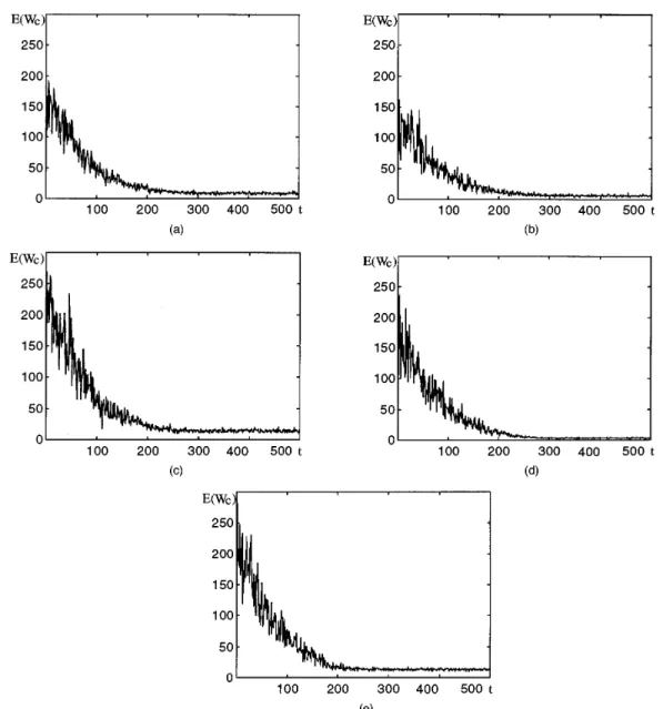
The blurred images and the restored images are shown in Figs. 5 to 9. In part~a! of each figure, the blurred image is generated using different blur matrices where each row is assigned to a normalized 2-D ‘‘noisy’’ Gaussian function where the noise is set to white and random with a strength of 30-dB SNR. The images from Fig. 3 degraded by 9 39 and 737 blur functions are shown in Fig. 5~a! and Fig. 6~a!, respectively. The image of Fig. 3 degraded by 737 blur functions in presence of noise at 30 dB SNR is shown in Fig. 7~a!. The image of Fig. 4 degraded by 737 blur functions is shown in Fig. 8~a!. The image of Fig. 4 de-graded by 737 blur functions in presence of noise at 30 dB SNR is shown in Fig. 9~a!. Part ~b! of each figure shows the restored image. The average computation time costs 1.17 h for each case. The learning curves for the five cases are shown in Figs. 10~a! to 10~e!. The averaged values of Fig. 4 Image of Fig. 3 degraded by white Gaussian noise at 20 dB

SNR.

Fig. 5 (a) Image of Fig. 3 degraded by 939 blur functions and (b) restored image for the degraded image in (a). The value ofDSNRis

9.8068.

Fig. 6 (a) Image of Fig. 3 degraded by 737 blur functions and (b) restored image for the degraded image in (a). The value of_DSNRis 3.3094.

Fig. 7 (a) Image of Fig. 3 degraded by 737 blur functions in pres-ence of white Gaussian noise at 30 dB SNR and (b) restored image for the degraded image in (a). The value ofDSNRis 3.2535.

E(Wc) for all xs are plotted to display the learning

behav-ior.

The convergence rate is related to the setup of the train-ing parameters, includtrain-ing the total iterations, the adaptation

rate, and the neighborhood function. In all our simulations, the weight matrices are always converged and approximate the true blur functions. The learning curves are always de-clined and stabilized after certain iterations. During each Fig. 8 (a) Image of Fig. 4 degraded by 7₃7 blur functions and (b)

restored image for the degraded image in (a). The value ofDSNRis

7.6621.

Fig. 9 (a) Image of Fig. 4 degraded by 737 blur functions in pres-ence of white Gaussian noise at 30 dB SNR and (b) restored image for the degraded image in (a). The value ofDSNRis 5.7993.

iteration, we calculate the averaged values of E(Wc) over

all sample input to indicate the goodness of the training results. The convergence rate is mainly related to the vari-ance of the image data and the initialization of the weight matrices.

SNR improvement is a popular measurement for the res-toration performance. SNR improvement is defined as DSNR510 log10

(siys2xsi2

(siys2yˆsi2

, ~14!

whereiys2xsi measures the distance between the sampled

blurred data xs and its corresponding original image data

ys, and iys2yˆsi measures the distance between the

re-stored data yˆsand the original image data ys. In the

simu-lations, SNR improvements for the five cases are 9.8068, 3.3094, 3.2535, 7.6621, and 5.7993, respectively.

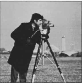
To compare with other methods, this approach is tested with the standard 2563256 8-bit monochrome cameraman image~Fig. 11!. Figure 12 shows the ‘‘Cameraman’’ image degraded by additive white noise at 30 dB SNR. There are 16316 neurons in the network. Each neuron has a 49 349-dimensional weight matrix. In this case, N516 and m15m257. The blurred images and the restored images

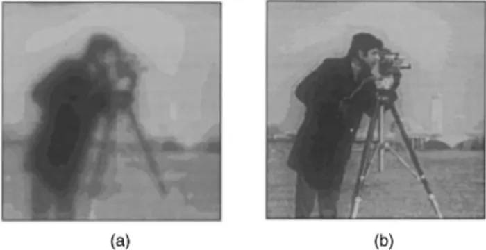
are displayed in Figs. 13 to 17. The noise in the 2-D Gauss-ian blur function is set to white and random with strength 40 dB SNR. The images from Fig. 11 degraded by 535 blur functions and 333 blur functions are shown in Fig. 13~a! and 14~a!, respectively. The image of Fig. 11 de-graded by 333 blur functions in presence of noise at 40 dB SNR is shown in Fig. 15~a!. The image of Fig. 12 degraded by 333 blur functions is shown in Fig. 16~a!. The image of Fig. 12 degraded by 333 blur functions in presence of noise at 40 dB SNR is shown in Fig. 17~a!. Part ~b! of each figure shows the restored image. The SNR improvements for the five cases are 8.4989, 4.0347, 4.0285, 4.1148, and 4.0756, respectively. The average computation time costs 3.25 h for each case.

Comparisons are also made with the results produced using other existing methods. These methods include in-verse filters, Wiener filters, constrained least squares, Kal-man filters, and constrained adaptive restoration.13 These are classical deblurring methods. The types of blur func-tions are known a priori in these methods. The SNR im-Fig. 11 Original 2563256 8-bit ‘‘Cameraman’’ image.

Fig. 12 Image of Fig. 11 degraded by white Gaussian noise at 30 dB SNR.

Fig. 13 (a) Image of Fig. 11 degraded by 535 blur functions and (b) restored image for the degraded image in (a). The value ofDSNR

is 8.4989.

Fig. 14 (a) Image of Fig. 11 degraded by 333 blur functions and (b) restored image for the degraded image in (a). The value ofDSNR

provements of the blurred cameraman image for each method are listed in Table 1 for comparisons.

From the simulation results, this approach is robust to the noise in either the observation process, the blur func-tion, or the image data. Comparing the restored results in Fig. 6~b! with those in Figs. 7~b! and 8~b!, we find that the noise in the observation process ~at 30 dB SNR! causes more difficulty in restoration than the noise in the image data~at 20 dB SNR!. Furthermore, this approach has larger SNR improvements for the cases without the observation noise.

In deriving the learning rule, we attempt to reduce the observation noise. The best-matching neuron c for input xs

is the neuron that has the minimum E(Wi)2log(Rˆi) value.

This E(Wi) is the distance between xsandWiyˆs.

Minimiz-ing this E(Wi) will reduce the observation noise optimally.

The neuron with the minimum E(Wi) value may not win

the competition. Hence the learning rule is not the optimal rule for reducing the observation noise. The value Rˆi,

which is used to estimate the a priori probability p(Wi), is

introduced in the term E(Wi)2log(Rˆi) by Eq.~4!. This Rˆi

makes the degraded image with the observation noise dif-ficult to restored. We may prefer the neurons with equal probabilities to improve the performance.

Acknowledgment

This work has been supported by the National Science Council, ROC.

References

1. T. G. Stockham, Jr., T. M. Cannon, and R. B. Ingebretsen, ‘‘Blind deconvolution through digital signal processing,’’ Proc. IEEE 63~4!, 678–692~1975!.

2. H. C. Andrews, ‘‘Digital image restoration: a survey,’’ Computer

7~5!, 36–45 ~1974!.

3. A. M. Tekalp, H. Kaufman, and J. Woods, ‘‘Identification of image and blur parameters for the noncausal blurs,’’ IEEE Trans. Acoust. Speech Signal Process. 34, 963–972~1986!.

4. G. R. Ayers and J. C. Dainty, ‘‘Iterative blind deconvolution method and its application,’’ Opt. Lett. 13~7!, 547–549 ~1988!.

5. B. C. McCallum, ‘‘Blind deconvolution by simulated annealing,’’ Opt. Commun. 75~2!, 101–105 ~1990!.

6. D. Kundur and D. Hatzinakos, ‘‘A novel recursive filtering method for blind image restoration,’’ in Proc. IASTED Int. Conf. on Signal and Image Processing, pp. 428–431~1995!.

7. R. A. Wiggins, ‘‘Minimum entropy deconvolution,’’ Geoexploration

16, 21–35~1978!.

8. M. K. Nguyen and A. Monhammad-Djafari, ‘‘Bayesian approach with the maximum entropy principle in image reconstruction from micro-wave scattered field data,’’ IEEE Trans. Pattern Anal. Mach. Intell. 6, 721–741~1984!.

9. T. Kohonen, Self-Organization and Associative Memory, Springer-Verlag, Berlin~1984!.

10. H. C. Andrews and B. R. Hunt, Digital Image Restoration, Prentice-Hall, Englewood Cliffs, NJ~1977!.

11. S. Geman and D. Geman, ‘‘Stochastic relaxation, Gibbs distributions and the Bayesian restoration of images,’’ IEEE Trans. Pattern Anal. Mach. Intell. 6, 721–741~1984!.

12. T. Kohonen, ‘‘Generalizations of the self-organizing maps,’’ in Proc. Int. Joint Conf. on Neural Networks, pp. 457–462, Japan~1993!. 13. J. Biemond, L. Lagendijk, and R. M. Mersereau, ‘‘Iterative methods

for image deblurring,’’ Proc. IEEE 78~5!, 856–883 ~1990!. 14. D. Kundur and D. Hatzinakos, ‘‘Blind image deconvolution,’’ IEEE

Signal Process. Mag. 13~3!, 43–64 ~1996!. Fig. 15 (a) Image of Fig. 11 degraded by 333 blur functions in

presence of white Gaussian noise at 40 dB SNR and (b) restored image for the degraded image in (a). The value of_DSNRis 4.0285.

Fig. 16 (a) Image of Fig. 12 degraded by 3₃3 blur functions and (b) restored image for the degraded image in (a). The value ofDSNR

is 4.1148.

Fig. 17 (a) Image of Fig. 12 degraded by 333 blur functions in presence of white Gaussian noise at 40 dB SNR and (b) restored image for the degraded image in (a). The value ofDSNRis 4.0756.

Table 1 Restoration performance for different methods.13

Methods _DSNR

Inverse Filters ₂16.5

Wiener Filters 5.9

Constrained Least Squares 6.2

Kalman filters 5.6

Constrained Adaptive Restoration 8.1

Cheng-Yuan Liou received the BS de-gree in physics from National Central Uni-versity in 1974, the MS degree in physical oceanography from National Taiwan Uni-versity in 1978, and the PhD degree in ocean engineering from the Massachu-setts Institute of Technology in 1985. From 1986 to 1987, he was a visiting associate professor in the Institute of Applied Me-chanics, National Taiwan University, where he taught courses in stochastic pro-cess and digital signal propro-cessing and did research in sonar array signal processing. In 1988, he joined the faculty of the same univer-sity, where he is currently a professor in the Department of Com-puter Science and Information Engineering. His current interests in-clude neural networks, digital signal processing, and artificial life.

Wen-Pin Tai received the BS degree, MS degree and PhD degree in computer sci-ence and information engineering from National Taiwan University in 1990, 1992, and 1997, respectively.