運用類自然語言處理之類神經網路預測分子與材料性質

全文

(1)國立臺灣大學工學院化學工程學系學士班學生論文 Department of Chemical Engineering College of Engineering. National Taiwan University Bachelor Degree Thesis. 運用類自然語言處理之類神經網路預測分子與材料性質 An Artificial Neural Network for Molecular and Material Properties Prediction Inspired by Natural Language Processing. 呂紹維 Shao-Wei Lu 指導教授：林祥泰博士 Advisor: Shiang-Tai Lin, Ph.D. 中華民國 109 年 6 月 June 2020.

(2)

(3) 中文摘要預測分子或材料的性質，一直是在科學研究上很被重視的課題，舉凡特用化學品的開發或者新藥的設計都與這個主題有關。理論上可以透過量子化學或者統計熱力學，來得到分子的性質，但因為多電子系統的薛丁格方程式並沒有解析解，要用近似的方法會消耗很多計算資源以及時間。因此所謂的定量結構與性質關係(QSPR)的模型就被提出，我們透過特徵工程將分子的結構轉換成描述子或者特徵，再透過數學上的方法將特徵與性質間的關係建立起來。隨著機器學習的發展，有越來越多用不同的機器學習技術，例如支援向量機或者隨機森林，來連結特徵與性質關係間的模型被提出。本論文建立在這樣的基礎上，受到語言翻譯的啟發，提出了另外一種預測分子性質的途徑。語言翻譯時，會建立一個語意空間(semantic space)，不同的語言可以藉由這個空間轉換。因此我們也相信存在有一個高維度的空間，它蘊含了用來描述分子最重要的資訊，從這個空間可以得到所有分子的性質。本論文利用 SMILES 以及 σ-profile 兩種不同的分子描述方法 (molecular representation)作為類神經網路的輸入，我們驗證利用類神經網路將分子描述法投射到這個空間，再從這個空間來預測分子的性質是可行的。此外我們也驗證了進行機器學習時，訓練集和測試集內資料的分布的選擇的重要。以及遇到過擬合(overfitting)的問題時，可以透過集成方法(ensemble method)來解決。我們也發現不同的分子表示法，會影響到模型的表現。 SMILES 的表現會比 σ-profile 來的好，因為 σ-profile 是從 SMILES 經過初步的量子化學計算得到的，這個過程就像是建立在人類智慧上的特徵工程，而透過類神經網路投影到高維度空間的過程則是建立在人工智慧上的特徵工程。在進行語言翻譯時，我們可以透過類神經網路將不同語言中對應到的字投影到語意空間。我們相信每種分子表示法或者性質，都可以理解成是分子的語言，因此我們的最終目標是同時透過多種分子表示法以及性質，來找到假設中的高維空間，如此一來，所有的分子性質都可以藉由這個空間來做到雙向的轉換。. II.

(4) Abstract Predicting molecules/material properties is always important when designing new drugs or developing novel material. Traditionally, we can acquire the properties from quantum mechanics or statistical thermodynamics. However, this process is time-consuming and resources-consuming. Therefore, the quantitative structure property relationship (QSPR) is proposed. This method converts structure into descriptors or features by feature engineering. Then map the relationship between features and property by the mathematical model or machine learning technique. This paper builds on this basis, we verify that using neural networks to extract latent features from different molecular representations and predicting properties from these latent features is feasible. Besides, we find that if the distribution of molecular size in the training and test set has a large difference, the model only performs well in the training set and cannot generalized to the test set. The so-called overfitting situation happened, and an ensemble method is a powerful way to deal with this problem. Moreover, we compare the performance of two models based on different representations respectively. The results show that σ-profile is more physically meaningful than SMILES. This is because σ-profile is the result of feature engineering by human intelligence of SMILES. Most importantly, we inspired by natural language translation. The process of language translation projects different words into semantic space then transforms between different languages. We believe any kind of property or representation can be viewed as a molecular language and there exists a hypothetical space contains all the necessary information about the molecules. All the properties of molecules can be derived from this space. We have verified that it is feasible to find this space from SMILES and σ-profile by neural network respectively. Therefore, our ultimate goal is to find this hypothetical space from multiple molecular representations and properties simultaneously. Then, we can bidirectionally transform between different properties and representations.. Keywords: Machine Learning, Natural Language Processing, Auto-encoder, Artificial Neural Network, Feature Engineering, Molecular Representations, Molecular Properties. III.

(5) 目錄 Table of Contents 口試委員會審定書………………………………………………………………………………. I. 中文摘要………………………………………………………………………….……………… II Abstract…………………………………………………………………………………………. III. 目錄 Table of Contents…………………………………………………………..……………. IV. 圖目錄 List of Figure…………………………………………………………………………… V 表目錄 List of Table…………………………………………………………………………… VI 1. 2.. 3. 4.. 5.. 6. 7. 8.. Introduction……………………………………………………………………………… Theory……………………………………………………………………………………… 2.1 Machine Learning……………………………………………………………………. 1 3 3. 2.2. Procedure of Machine Learning……………………………………………………… 2.2.1 Training, Validation, and Test Set…………………………………………… 2.2.2 Structure of the Neural Network…………………………………………… 2.2.3 Definition of the Loss Function…………………………………………… 2.2.4 Optimizer: Gradient Descent and Backpropagation…………………………. 2.3 2.4 2.5 2.6. Overfitting and Solutions…………………………………………………………… 8 DNN and RNN……………………………………………………………………… 9 Auto-encoder………………………………………………………………………… 10 Molecular Representation…………………………………………………………… 10 2.6.1 SMILES……………………………………………………………………… 11. 3 4 4 6 7. 2.6.2 σ-profile……………………………………………………………………… Databases………………………………………………………………………………… Computational Details…………………………………………………………………… 4.1 One-Hot Encoding and Vectorized SMILES……………………………………… 4.2 Vectorized σ-profile…………………………………………………………………. 11 12 13 13 13. 4.3 Structure of the Model……………………………………………………………… Result and Discussion…………………………………………………………………… 5.1 Different Distribution of Molecular Size…………………………………………… 5.2 Overfitting and the Ensemble Method………………………………………………. 13 15 18 18. 5.3 Different Type of Molecular Representations……………………………………… Conclusion………………………………………………………………………………… Future Work……………………………………………………………………………… References…………………………………………………………………………………. 18 20 21 22. IV.

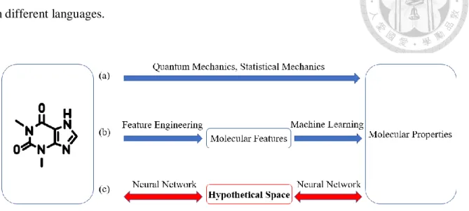
(6) 圖目錄 List of Figure Figure 1.. Different approaches to acquire molecular properties. (a) traditional methods (b) chemoinformatics models (c)neural network inspired by natural language translation………………………………………………………. 2. Figure 2. The difference between (a) traditional machine learning and (b) deep learning…….. 3. Figure 3.. The architecture of the neural network. ……………………………………………. 4. Figure 4.. A basic unit (neuron) in the neural network. ………………………………………. 5. Figure 5.. Different types of activation function. ………………………………………………. 5. Figure 6.. The schematic overview of gradient descent. ………………………………………. 7. Figure 7.. The schematic overview of underfitting and overfitting situation. …………………. 8. Figure 8.. Loss during the training process. ……………………………………………………. 9. Figure 9.. The schematic overview of ensemble method. ……………………………………… 9. Figure 10. The architecture of the auto-encoder. ……………………………………………… 10 Figure 11. Different representations of a same molecule. ……………………………………. 11. Figure 12. SMILES_logP and σ_logP model. …………………………………………………. 14. Figure 13. SMILES_logP model results on test data of GDB-11 database. …………………… 16 Figure 14. SMILES_logP model results on test data of GDB-11 database (ensemble). ………. 16. Figure 15. SMILES_logP model results on test data of Sigma database. ……………………… 17 Figure 16. σ_logP model results on test data of Sigma database………………………………. 17. Figure 17. The concept of language and molecular translation. ………………………………… 21. V.

(7) 表目錄 List of Table Table 1. Training set and test set of GDB-11 and Sigma databases…………………………… 12 Table 2. Results of SMILES_logP model on GDB-11 database………………………………. 16. Table 3. Results of SMILES_logP model on GDB-11 database (ensemble) …………………. 16. Table 4. Results of SMILES_logP model on Sigma database………………………………… 17 Table 5. Results of σ_logP model on Sigma database………………………………………… 17. VI.

(8) 1. Introduction Nowadays, there are more and more efforts dedicated to developing specialty chemicals, novel materials, and innovative drugs. When dealing with the abovementioned tasks, it is necessary to acquire molecular properties from its structure. From Figure1(a)., traditionally, we can use methods of quantum chemistry and statistical mechanics to obtain desired quantum or thermodynamic properties. However, the difficulty is that Schrödinger's equation for the multi-electronic system has no analytical solution and the approximation method will consume considerable computing resources and time. Additionally, it is annoying and inefficient to repeat calculation whenever we encounter new molecules. According to the above discussion, the most ideal method to acquire molecular properties is to derive a model based on existing data, then using it to predict the properties of new molecules. To achieve the above goal, we want to get help from the thriving of artificial intelligence and machine learning. We take advantage of neural networks to build a mathematical model based on sample molecules along with known properties, in order to predict new molecules. From Figure1(b)., the so-called chemoinformatics model is the study of this kind of approach1-7. The model consists of two parts. First, a molecular structure is converted into a vector of features, which also known as the descriptors. This process is called feature engineering. Next, we map the feature vector to the interested properties. The mapping process finds the underlying function and pattern which generally based on machine learning techniques. The most efforts of this approach put on finding different combinations of features vector and machine learning techniques. For example, Wu, Zhenqin et al. (2018) compared the performance of many different featurization methods, such as extended circular fingerprints (ECFP)8, coulomb matrix, and graph convolution with different machine learning technique, such as random forest and neural network on the same database9. Jeon, Woosung et al. (2019) proposed a new featurization method based on neural networks to enhance the performance of the chemoinformatics model10. In this paper, we inspired by the concept of language translation11 and propose another approach rather than focusing on extracting features then mapping it to properties. During language translation, each word will project to a high dimensional space called semantic space. Each corresponding word in different languages will project to the same point in this space. So, we assume there exists a hypothetical space that contains all the necessary information of the molecule, for instance, the wave function in quantum mechanics and the partition function in statistical mechanics. Besides, we think different molecular properties can be viewed as different languages of molecules. Therefore, we believe that all the properties of a molecule/material can be properly derived from this hypothetical 1.

(9) space. Form Figure 1(c)., our ultimate goal is to find that space using multiple molecular/material properties simultaneously by the neural network. Just like finding the semantic space of each word from different languages.. Figure 1. Different approaches to acquire molecular properties. (a)traditional methods (b) chemoinformatics models (c)neural network inspired by natural language translation. Our approach is more efficient than traditional quantum mechanics methods, because we can directly use the model when we encounter new molecules rather than consume lots of resources and time. Besides, we can bidirectionally transform between different molecular properties and representations from the hypothetical space. While most chemoinformatics model only map the unidirectional relationship between structure and property.. 2.

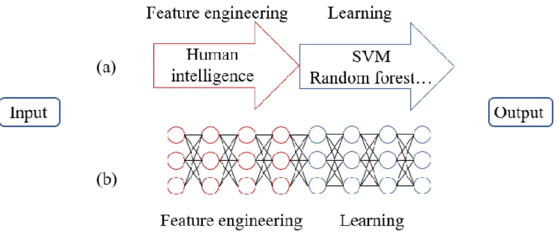
(10) 2. Theory 2.1 Machine Learning Machine learning12-13 is a way to achieve artificial intelligence. It is the study of algorithm and statistical model that computer systems use to perform a specific task relying on patterns and inference rather than explicitly instructing and programming. As for deep learning 14-15, it is a branch of machine learning. It using deep neural networks to achieve the goal of machine learning. When doing conventional machine learning techniques, most efforts are put on feature engineering. From Figure 2(a)., it means extracting important features from original data that need domain knowledge and rely on human intelligence. Then use traditional methods such as support vector machine (SVM)16 or random forest17 to learn the pattern. The goal and advantage of deep learning is to realize end-to-end learning. As shown in Figure 2(b)., it means the neural network performs feature engineering itself. We believe each layer can act as a transformer or classifier. After many deep layers, the machine can perform feature engineering itself and learn the underlying pattern from training data for classification or regression problems.. Figure 2. The difference between (a) traditional machine learning and (b) deep learning.. 2.2 Procedure of Machine Learning The procedure to create a neural network model and train it by data can be simply divided into four steps. First, we need to collect data or find the source of data and split it properly. Next, we should determine the structure of the neural network. Such as the number of neurons and layers and the type of activation function. Then, we define the loss function which measures the error between the predicted value and the expected value. After that, we choose the optimizer which means the most suitable algorithm to optimize the model parameters to get the best performance. In the next part, we 3.

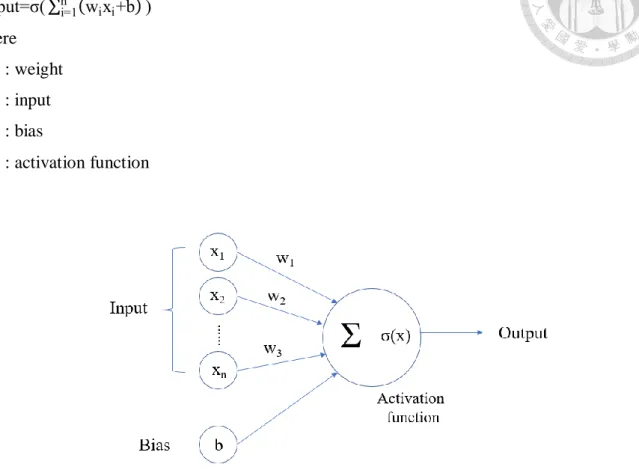
(11) will introduce these four steps in detail.. 2.2.1 Training, Validation, and Test Set After finding the source or collecting a group of data, we will split it into the training set, validation set, and test set. The training set is simply used to train a neural network, in other words, tuning the parameters of the model. The function of the test set is acting as new data which used to judge the performance of the trained model. Our ultimate goal is to develop a model that can generalize to new data. Excellent performance on the training set does not guarantee the equivalent performance on the test data. Therefore, there comes up with a concept called the validation set. The model sees the validation set but does not learn from it. It acts as pseudo-test data deciding which group of parameters is the most suitable. The process is called fine-tuning. That is, make the training set and validation set have the optimal performance simultaneously. Therefore, we can generalize this model to test data and expect good performance.. 2.2.2 Structure of the Neural Network A neural network is composed of the input layer, hidden layer, and output layer. Each layer consists of a group of nodes. Node, or neuron is the basic unit of the neural network.. Figure 3. The architecture of the neural network.. Each node will receive the previous output as its input and generate the output after proper transformation. As shown in Figure 4. and Equation (1), the output of a neuron is determined by the output of the previous layer, weight, bias, and the activation function. The output in the previous layer will be multiplied by so-called weights then add it together with bias. Next, transforming by an 4.

(12) activation function to get the output of this neuron. output=σ( ∑ni=1 (wi xi +b) ). (1). where w. : weight. x. : input. b. : bias. σ. : activation function. Figure 4. A basic unit (neuron) in the neural network.. The basic idea of the activation function is to simulate the opening and closing of neural signals. With the development of different types of neural networks and algorithm, more different versions of activation functions are proposed. Figure 5. shows some of them.. Figure 5. Different types of activation function.. 5.

(13) The parameters of the neural network model are weights and bias. We will tune the parameters so that the model has the best performance. The word deep in deep learning means many layers are stacked together. The whole structure of neural networks can be viewed as a non-linear function. Data is read by the neural network from the input layer. Then, after transformed by a set of weights, bias, and activation function in the hidden layer, the result of regression or classification is expressed in the output layer. By tuning the value of weights and bias from the training data, this neural network not only maps the input to output, but also learn and reveal the underlying physical laws, or so-called patterns.. 2.2.3 Definition of the Loss Function The metric used to measure the difference between the expected value and predicted value from neural networks is called the loss function. There have lots of options and we can even define it by ourselves. Different loss function will be selected in different task. If an inappropriate loss function is used, it will result in an ineffective training process and lead to terrible performance. Give a few common examples, cross entropy and mean square error. The concept of cross entropy comes from information theory, it used to compare the similarity between two different probability distributions. So cross entropy is dominant when we treat a classification problem. Because the principle of classification is to predict the possibility of each possible outcome. The smaller the value of cross entropy, the similar the two probability distributions. For two identical probability distribution, the cross entropy of them is 0. H(p,q)= - ∑x∈X p(x) ln q(x). (2). Where p. : actual probability distribution. q. : predicted probability distribution. x. : each possible outcome in the probability distribution. X. : set of possible outcomes in the probability distribution. When the task is about regression, the mean square error is very common and useful. The smaller the value of mean square error, the more accurate the model predicts.. 6.

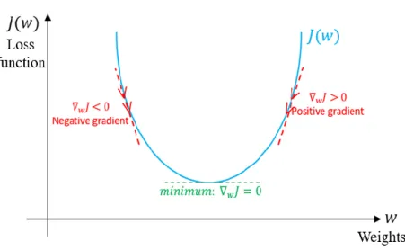
(14) MSE=. 1 N. ∑N ̂ )2 i=1 (y-y. (3). Where y. : predicted value. 𝑦̂. : expected value. 2.2.4 Optimizer: Gradient Descent and Backpropagation After defining the loss function, we need to minimize it by tuning the parameters of the model. Because the output of the neural network is obtained after a series of operations of weights and bias, the loss function will contain the above parameters. Here comes the concept called gradient descent, it iteratively moving in the direction of steepest descent as defined by the negative of the gradient, looking forward to finding the globe minimum. Wi+1 = Wi -λ∇J(Wi ). (4). Where Wi+1. : weight after update. Wi. : weight before update. ∇J(Wi ) : gradient of loss function when the parameter is Wi λ. : learning rate. Figure 6. The schematic overview of gradient descent.. Figure 6. shows the process to reach the global minimum. The learning rate determines the rate or 7.

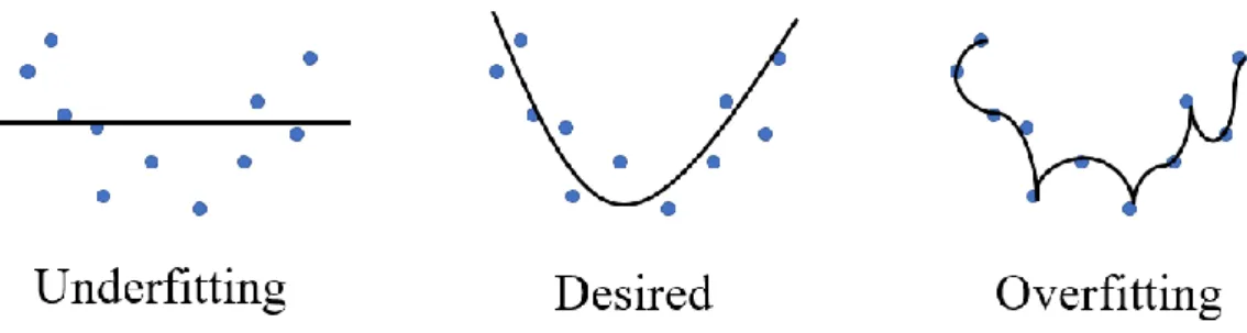
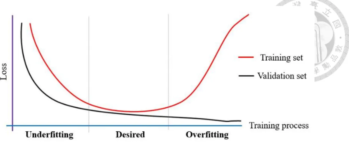
(15) magnitude of updating parameters. If it is too low, the optimization process may stuck in the saddle point or local minimum. On the other hand, if the learning rate is too large, it may move back and forth between the global minimum. The most commonly used minimum algorithms are based on gradient descent, such as Adagrad18 and Adam. They all propose some correction term or modify the learning rate to improve the process of optimizing parameters. In the process of gradient descent, we need to calculate the partial derivative respective to each weight and bias. Because the neural network is so deep, we used the so-called backpropagation method to realize the complex process of chain rule from back to front.. 2.3 Overfitting and Solutions As mentioned above, it is easy to iterate too many times during the optimization process leading to over-optimize the parameters. It causes a complex model so that the model has very little error in the training set, but the performance is very poor when we want to generalize this model to the test set. This situation is called overfitting. On the other hand, if we don’t have enough iterations to optimize the parameters, the over-simplified model will not learn anything from the training data. It will have poor performance on both training data and test data. This situation is called underfitting. So, there is always a trade-off between optimization and generalization. Too much emphasis on optimization will lead to overfitting, while too much focus on generalization will cause underfitting.. Figure 7. The schematic overview of underfitting and overfitting situation.. There are some ways to deal with the overfitting problem. We can monitor the loss function of the training set and validation set during the training process. When the loss of the training set is decreasing while that of the validation set is increasing, it means that the trained model is too focus on the features and details of the training set. Overfitting has occurred. So, we stop the training process when both the training set and validation set have good performance simultaneously. This method is called the early-stopping. 8.

(16) Figure 8. Loss during the training process.. Moreover, we know overfitting comes from an over-complex model and this kind of model has little bias but a large variance. So, we use averaging to reduce the variance of the model. To realize this concept during training process, we trained many different models based on the same data. Use these models to predict, then averaging the prediction of each model to get the final results. This technique is called an ensemble method19-20.. Figure 9. The schematic overview of ensemble method.. 2.4 DNN and RNN We will slightly modify the architecture of the neural network for different tasks. Based on the deep neural network (DNN), we can further memory the present state and use it as one of the next inputs. So, we can not only process single data, but also a sequence of data. Then we have the so-called recurrent neural network (RNN)21-22. RNN is suitable for dealing with dynamic and sequential problems, such as speech reorganization. Because it is important for the continuous or sequential data to memory its previous state. The most commonly used RNN module is long short-term memory 9.

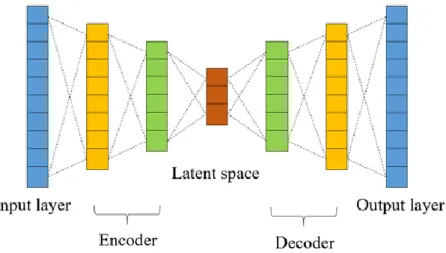
(17) (LSTM)23. A single unit of LSTM consists of input, output, and forget gates. The on/off of each gate is learned by the machine itself from the training data. By increasing the design of the gate, we can make the machine have memory.. 2.5 Auto-encoder The auto-encoder24 is a special type of neural network. It consists of encoder and decoder. The number of neurons in the encoder layers is decreasing while that in the decoder layers is increasing. We deliberately make the input and output of the auto-encoder the same. It means the input can convert back to the original representation after a series of transformations inside the hidden layer. So, we give the output of the middle layer or bottleneck layer a special name called latent features, which contain all the necessary and essential information about the original data.. Figure 10. The architecture of the auto-encoder.. This process can be viewed as a kind of dimension reduction. We discard redundant information and extract the essence through auto-encoder to get the so-called latent space which is more representative and informative.. 2.6 Molecular Representation Making computer and mathematical models understand the structure or the feature of molecules is an essential and crucial task. Furthermore, it’s often the key to the performance of the model. There are many ways to represent the type of atoms that forms a molecule and the connectivity between them on the computer. More broadly, the method of describing the electronic interaction of the molecular can also be called molecular representation. In this paper, we utilize two different molecular 10.

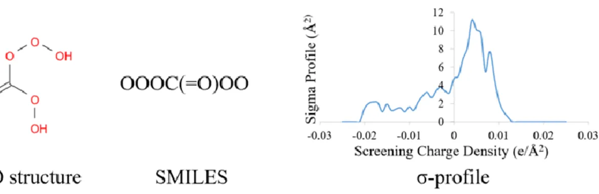
(18) representations and verify their performance.. 2.6.1 SMILES25 One simple way is Simplified Molecular Input Line Entry Specification (SMILES) which is a specification in the form of a line notation. SMILES uses the English alphabet to express the type of atoms and other symbols to express the connectivity between them. For example, the SMILES representation of acetic acid is CC(=O)O. English letter C means the carbon atom, while character = means the double bond between carbon and oxygen. Besides, character () means the side chain.. 2.6.2 σ-profile A more advanced method is called σ-profile. This concept comes from the COSMO-based model. Conductor-like Screening Model (COSMO)26 is a calculation method for determining the electrostatic interaction of a molecule with a solvent. And σ-profile is the probability distribution of surface area having specific screening charge density σ (e/Å2). Because the generation of σ-profile needs preliminary quantum calculation based on the type of atoms and connectivity, it describes the electronic interaction of the molecular. Therefore, σ-profile can better represent the characteristics of the molecules theoretically. Following is an example of different molecular representation of the same molecule.. Figure 11. Different representations of a same molecule.. 11.

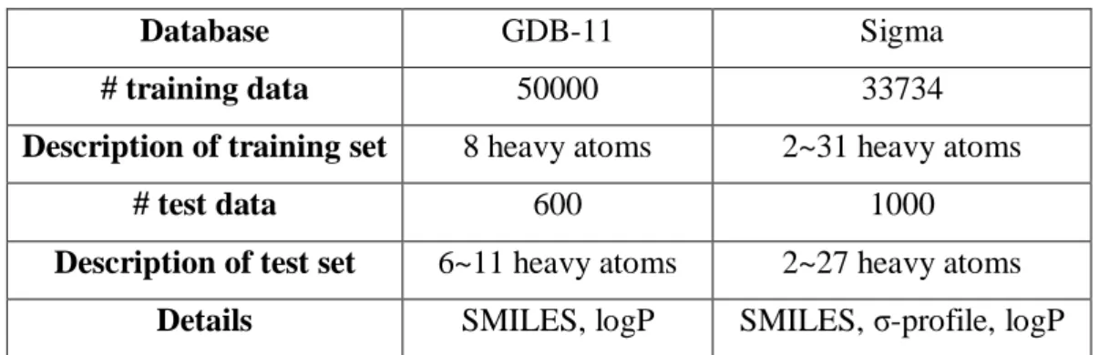
(19) 3. Databases As mentioned early, we need sample molecules to train the neural network model and new molecules to test the performance of the model. Hence, we choose two molecular databases as our source of molecules, one is GDB-1127-28 and the other is Sigma database. GDB-11 is a database which collects small organic molecules up to 11 atoms of C, N, O, and F following simple chemical stability and synthetic feasibility rules. GDB-11 database is expressed in the form of SMILES. Other than that, Sigma database is build up by our lab which consists of molecules ranging from 2~31 heavy atoms (except for hydrogen). In addition to SMILES, the Sigma database also records the σ-profile of each molecule. Therefore, there are two type of molecular representations can be used to train the neural network as input. As for the output, we choose the n-octanol/water partition coefficient (logP) as interested property in this paper. It is the ratio of concentrations of such compounds in a mixture of two immiscible solvents at equilibrium. We utilizing RDKit, an open-source cheminformatics software to calculate the n-octanol/water partition coefficient as our expected output when training the model. Besides, as mentioned above, we split each database into different sets to train, validate, and test. In this paper, actually, we divide the database into the training set and test set, then using 30 percent of training data to validate the model and avoid overfitting. In the GDB-11 database, we deliberately make the distribution of molecular size different in the training set and test set. In detail, we only choose molecules that contain 8 heavy atoms as our training set, and molecules that contain 6~11 heavy atoms as our test set. On the other hand, we make the distribution of molecular size in the training set and test set of the Sigma database roughly the same. The most frequently occurring molecular size is 7, and the percentage is 32.5% in both training set and test set. We want to verify whether the distribution of molecular size inside the training set and test set will affect the performance of the model.. Table 1. Training set and test set of GDB-11 and Sigma databases Database. GDB-11. Sigma. # training data. 50000. 33734. Description of training set. 8 heavy atoms. 2~31 heavy atoms. # test data. 600. 1000. Description of test set. 6~11 heavy atoms. 2~27 heavy atoms. Details. SMILES, logP. SMILES, σ-profile, logP. 12.

(20) 4. Computational Details 4.1 One-Hot Encoding and Vectorized SMILES When training the neural network, everything is represented by vector rather than alphabet or character. So, we borrow the concept of one-hot encoding which is often used in natural language processing to encrypt SMILES representation. We create a vector which element represents the alphabet or character that has appeared in the training data. The vector consists of 0 in all elements with the exception of a single 1 in an element used uniquely to identify the alphabet or character. From another perspective, this vector represents the probability distribution of each alphabet or character. After the transformation, a matrix which size is m×n is used to represent a molecule. Where m is the largest number of alphabet and character owned by a molecule in the training set and n is the total number of alphabet or character appeared in the training set.. 4.2 Vectorized σ-profile It is observed that the screening charge density for most molecules lies between -0.025 to 0.025 (e/Å 2). When we choose the interval as 0.001, we can use a vector which has 51 elements to represent a molecule. The value of each element is the molecular area under that specific screening charge density. This vector which has 51 elements will serve as our input to the neural network.. 4.3 Structure of the Model Our fundamental idea is to use auto-encoder to extract latent features from different molecular representations. In other words, project molecular representation into more informative latent space. Because we believe this latent space contains all the essential information about the molecule, we use these latent features to predict the molecular properties. Therefore, our structure of the model is made up of two parts. One is an auto-encoder to extract the essential features and the other is a neural network to predict logP form these latent features. We create two types of models using SMILES and σ-profile as input, and we call it SMILES_logP29 and σ_logP model respectively. The difference between the two models is the input representation, the architecture of the auto-encoder, and the selection of the loss function. Because SMILES representation expresses the sequential relationship and connectivity between atoms, so we choose RNN architecture which is suitable for handling sequential data as our autoencoder in the SMILES_logP model. As for σ-profile, we simply choose DNN architecture as our auto-encoder. 13.

(21) Figure 12. SMILES_logP and σ_logP model.. When we encrypt SMILES into one-hot encoding then using auto-encoder to extract the latent feature, the value of each element in this vector actually represents the probability. So it is a classification problem and the loss function we chose is cross entropy. While the value of each element in the σprofile vector represents the real molecular area. Therefore, we choose the mean square error as our loss function. In addition, the part of predicting logP from latent features in both models is a regression problem. So again, mean square error is the most suitable loss function. Besides, the optimizer we chose in this paper is Adam, which is the most commonly used algorithm with the best performance.. 14.

(22) 5. Results and Discussions First, this paper uses SMILES_logP model on both GDB-11 and Sigma databases to verify the effect of molecular size distribution in the training and test set on the neural network. Besides, we use the ensemble method to solve overfitting problem. Furthermore, we also use SMILES_logP and σ_logP model on Sigma database to compare the performance of two different molecular representations. In the following table, Loss_1 means the average loss when the auto-encoder extracting the latent features, while Loss_2 means the average loss of the neural network predicting logP from latent feature during the training process. As mentioned above, we choose cross entropy for SMILES autoencoder but MSE for σ-profile autoencoder. As for the performance on test data, we select root mean square error (RMSE) and correlation coefficient R2 as our metrics. We expect the smaller the RMSE and the closer to 1 the R2.. 1. RMSE= √N ∑N ̂ )2 i=1 (y-y. R2 =(. n ∑(yŷ )-(∑ y)(∑ ŷ ) √[n ∑(y2 )-(∑ y)2 ][n ∑(ŷ 2 )-(∑ ŷ )2]. (5). ). 2. (6). where y. : predicted value. 𝑦̂. : expected value. 15.

(23) Table 2. Results of SMILES_logP model on GDB-11 database Database. GDB-11. Model. SMILES_logP. Loss_1. Loss_2. (cross entropy). (MSE). 0.0018. 0.1389. RMSE. R2. 0.9461. 0.4660. Figure 13. SMILES_logP model results on test data of GDB-11 database.. Table 3. Results of SMILES_logP model on GDB-11 database (ensemble) Database. GDB-11. Model. SMILES_logP. Loss_1. Loss_2. (cross entropy). (MSE). Ensemble method. RMSE. R2. 0.4076. 0.8433. Figure 14. SMILES_logP model results on test data of GDB-11 database (ensemble). 16.

(24) Table 4. Results of SMILES_logP model on Sigma database Database. Sigma. Model. SMILES_logP. Loss_1. Loss_2. (cross entropy). (MSE). 0.0340. 0.3478. RMSE. R2. 0.5741. 0.7989. Figure 15. SMILES_logP model results on test data of Sigma database Table 5. Results of σ_logP model on Sigma database Database. Sigma. Model σ_logP. Loss_1. Loss_2. (MSE). (MSE). 3.4306. 0.2709. RMSE. R2. 0.5177. 0.8362. Figure 16. σ_logP model results on test data of Sigma database 17.

(25) 5.1 Different Distribution of Molecular Size From Figure 13., we find that the trained model will have different performance when predicting molecules of different sizes. For molecules having 8 heavy atoms, the predicted value and expected value roughly lie on the diagonal. While molecules having 10 and 11 heavy atoms have large deviation. The reason why the trained model performs best when predicting molecules of 8 heavy atoms is the training set we choose. We deliberately let the training set only contain molecules of 8 heavy atoms. So, we verify that machine really learns details and features only belong to molecules of such specific size. When we want to generalize the model to the molecules of different sizes, it falls. And the greater the difference in the size of molecules, the worse the performance. On the other hand, from Figure 15., we find the trained model performs roughly the same when predicting molecules of different sizes, except some special outliers. Because we make the distribution of molecular size in the training set broader and more diverse. Besides, we check the distribution of molecular size in the training set and test set is roughly the same. Therefore, the machine can learn more diverse and general features that belong to all size of molecules and we can get a more general model.. 5.2 Overfitting and the Ensemble Method When the trained model cannot generalize to molecules of different sizes, it means the overfitting situation happened. The machine learns specific and limited features rather than diverse and general features. Fortunately, we can use the ensemble method to deal with this problem. We train four different models with the same data. The predicted results between each model have a small bias but a large variance. Then we average the predicted values from each model as the final result. Theoretically, the averaging process can reduce the large variance and get better performance. From Figure 14., we find the ensemble method worked. We successfully solved the overfitting problem.. 5.3 Different Type of Molecular Representations We use two different types of auto-encoder on Sigma database. One uses SMILES as input and the other uses σ-profile as input. We want to verify which molecular representation can better express the molecules. Especially the electronic interaction, which determines most of the properties of a molecule. From Figure 15. and Figure 16., the results show that when we select σ-profile as our input, we can get better performance than SMILES. The reason is that σ-profile is obtained after preliminary quantum calculation. The electronic interaction of a molecule can be calculated form the type of atoms and connectivity between them after quantum calculation. SMILES only express the type of 18.

(26) atoms and connectivity between them, while σ-profile express the electronic interaction. Therefore, σ-profile can better represent a molecule than SMILES. From the perspective of machine learning, σ-profile is actually the results of SMILES after doing feature engineering by human intelligence. The process discard redundant information and obtain more representative expression.. 19.

(27) 6. Conclusion From above results, we come to a conclusion that the auto-encoder is a useful way to extract latent features from different molecular representations. Besides, using latent features to predict molecular properties is feasible. Furthermore, we believe the latent space contains all the necessary information about such molecule. Multiple properties can be bidirectionally transformed between each other. We also verify that the machine learns from what we give to it. Therefore, the split of database is important. The model does not work if the training set contains only the specific size of molecules. Before we actually utilize this model to predict the new molecules, we cannot confirm the size distribution of them. In most cases, it is assumed that this distribution is similar to the distribution of the test set. Therefore, we must make sure that the molecular size distribution in the training set is the same as test set. If the training set only contain specific molecules, the machine will learn limited features. As consequence, we cannot get general model, which means we have no way to predict molecules of different sizes. The trained model is useless. If it has too many iterations during the process of optimizing parameters to minimize the loss function, the model may over-focus on the specific details only belong to training data. It may lead to an overcomplex model and cause the over-fitting problem. In other words, we get a model that cannot be generalized in the trade-off between optimization and generalization. When this circumstance unfortunately happens, the ensemble method is a powerful method to deal with it. The reason why this method works is because overfitting is caused by an over-complex model. It has the characteristics of a low bias but a high variance. The process of averaging can reduce the variance and we expect to get better performance. Moreover, using σ-profile as a molecular representation will have better performance than SMILES. It is because σ-profile describes the electrostatic potential of the molecule by preliminary quantum calculation, while SMILES only express the type of atoms which made up the molecule and the connectivity between them. We know that most of properties of the molecule is determined by the electronic interaction of the molecule. Therefore, σ-profile is more physically meaningful and representative than SMILES. We know that feature engineering means discarding the redundant information then acquiring more representative expression. The process can be done by either human or artificial intelligence. Preliminary quantum calculation is feature engineering by human intelligence and the auto-encoder is feature engineering by artificial intelligence. The results show that if we do the feature engineering by human intelligence first, we can expect to get better performance.. 20.

(28) 7. Future Work The concern and criticism about machine learning lie in the so-called black box. We cannot clearly indicate what the machine has learned and why it makes such predictions. We believe we can solve this problem by further investigating the latent space. As mentioned above, this space contains and implies all the necessary and essential information about the molecules. We borrow the concept from natural language processing. When translating between different languages, there is a technique using RNN to project each word to a high dimensional space which we call it the semantic space. Each corresponding word in different language will project to the same point in this space. Therefore, we are inspired by language translation and propose so-called molecular translation. We believe there exists a high dimensional space that contains all the necessary information of the molecule, for instance, the wave function in quantum mechanics and the partition function in statistical mechanics. We believe that all the properties of a molecule/material can be properly derived from this space. We call this space the Schrödinger space. In this paper, we have used the auto-encoder to extract and project SMILES and σ-profile into Schrödinger space respectively. If we can prove that similar molecules will be in close positions in Schrödinger space no matter which representations or properties are used for auto-encoder to extract features, we can confirm that the machine really learned some underlying physical patterns and the assumption of Schrödinger space is feasible. Therefore, the criticism of black box can be explained.. Furthermore, we can even use multiple. properties and representations simultaneously to acquire a more accurate Schrödinger space. Therefore, we can effectively and bidirectionally convert between multiple molecular properties.. Figure 17. The concept of language and molecular translation.. 21.

(29) 8. References [1] Svetnik, V., Liaw, A., Tong, C., Culberson, J. C., Sheridan, R. P., & Feuston, B. P. (2003). Random forest: A classification and regression tool for compound classification and QSAR modeling. Journal of Chemical Information and Computer Sciences, 43(6), 1947-1958. [2] Dudek, A. Z., Arodz, T., & Galvez, J. (2006). Computational methods in developing quantitative structure-activity relationships (QSAR): A review. Combinatorial Chemistry & High Throughput Screening, 9(3), 213-228. [3] Varnek, A., & Baskin, II. (2011). Chemoinformatics as a Theoretical Chemistry Discipline. Molecular Informatics, 30(1), 20-32. [4] Varnek, A., & Baskin, I. (2012). Machine Learning Methods for Property Prediction in Chemoinformatics: Quo Vadis? Journal of Chemical Information and Modeling, 52(6), 1413-1437. [5] Mitchell, J. B. O. (2014). Machine learning methods in chemoinformatics. Wiley Interdisciplinary Reviews-Computational Molecular Science, 4(5), 468-481. [6] Ma, J. S., Sheridan, R. P., Liaw, A., Dahl, G. E., & Svetnik, V. (2015). Deep Neural Nets as a Method for Quantitative Structure-Activity Relationships. Journal of Chemical Information and Modeling, 55(2), 263-274. [7] Duvenaud, D. K., et al. (2015). Convolutional networks on graphs for learning molecular fingerprints. In: Advances in Neural Information Processing Systems (Vol. 28, pp. 2224-2232) [8] Rogers, D., & Hahn, M. (2010). Extended-Connectivity Fingerprints. Journal of Chemical Information and Modeling, 50(5), 742-754. [9] Wu, Z. Q., Ramsundar, B., Feinberg, E. N., Gomes, J., Geniesse, C., Pappu, A. S., . . . Pande, V. (2018). MoleculeNet: a benchmark for molecular machine learning. Chemical Science, 9(2), 513-530. [10] Jeon, W., & Kim, D. (2019). FP2VEC: a new molecular featurizer for learning molecular properties. Bioinformatics, 35(23), 4979-4985. [11] Turney, P. D., & Pantel, P. (2010). From Frequency to Meaning: Vector Space Models of Semantics. Journal of Artificial Intelligence Research, 37, 141-188. [12] Blum, A. L., & Langley, P. (1997). Selection of relevant features and examples in machine learning. Artificial Intelligence, 97(1-2), 245-271. [13] Butler, K. T., Davies, D. W., Cartwright, H., Isayev, O., & Walsh, A. (2018). Machine learning for molecular and materials science. Nature, 559(7715), 547-555. [14] LeCun, Y., Bengio, Y., & Hinton, G. (2015). Deep learning. Nature, 521(7553), 436-444. [15] Schmidhuber, J. (2015). Deep learning in neural networks: An overview. Neural Networks, 61, 85-117. 22.

(30) [16] Cortes, C., & Vapnik, V. (1995). SUPPORT-VECTOR NETWORKS. Machine Learning, 20(3), 273-297. [17] Breiman, L. (2001). Random forests. Machine Learning, 45(1), 5-32. [18] Duchi, J., Hazan, E., & Singer, Y. (2011). Adaptive Subgradient Methods for Online Learning and Stochastic Optimization. Journal of Machine Learning Research, 12, 2121-2159. [19] Dietterich, T. G. (2000). Ensemble methods in machine learning. In J. Kittler & F. Roli (Eds.), Multiple Classifier Systems (Vol. 1857, pp. 1-15). [20] Zhou, Z. H., Wu, J. X., & Tang, W. (2002). Ensembling neural networks: Many could be better than all. Artificial Intelligence, 137(1-2), 239-263. [21] Williams, R. J., & Zipser, D. (1989). A Learning Algorithm for Continually Running Fully Recurrent Neural Networks. Neural Computation, 1(2), 270-280. [22] Schuster, M., & Paliwal, K. K. (1997). Bidirectional recurrent neural networks. Ieee Transactions on Signal Processing, 45(11), 2673-2681. [23] Hochreiter, S., & Schmidhuber, J. (1997). Long short-term memory. Neural Computation, 9(8), 1735-1780. [24] Hinton, G. E., & Salakhutdinov, R. R. (2006). Reducing the dimensionality of data with neural networks. Science, 313(5786), 504-507. [25] Weininger, D. (1988). SMILES, A CHEMICAL LANGUAGE AND INFORMATIONSYSTEM .1. INTRODUCTION TO METHODOLOGY AND ENCODING RULES. Journal of Chemical Information and Computer Sciences, 28(1), 31-36. [26] Klamt, A., & Schuurmann, G. (1993). COSMO - A NEW APPROACH TO DIELECTRIC SCREENING IN SOLVENTS WITH EXPLICIT EXPRESSIONS FOR THE SCREENING ENERGY AND ITS GRADIENT. Journal of the Chemical Society-Perkin Transactions 2(5), 799805. [27] Fink, T., Bruggesser, H., & Reymond, J. L. (2005). Virtual exploration of the small-molecule chemical universe below 160 daltons. Angewandte Chemie-International Edition, 44(10), 1504-1508. [28] Fink, T. & Reymond, J. L. (2007). Virtual exploration of the chemical universe up to 11 atoms of C, N, O, F: assembly of 26.4 million structures (110.9 million stereoisomers) and analysis for new ring systems, stereochemistry, physico-chemical properties, compound classes and drug discovery. Journal of Chemical Information and Modeling, 47, 342-353. [29] Sattarov, B., Baskin, II, Horvath, D., Marcou, G., Bjerrum, E. J., & Varnek, A. (2019). De Novo Molecular Design by Combining Deep Autoencoder Recurrent Neural Networks with Generative Topographic Mapping. Journal of Chemical Information and Modeling, 59(3), 1182-1196. 23.

(31)