利用預棄技術和狀態再利用的技巧實現低功率渦輪解碼器

國

國

國

國 立

立

立

立 交

交

交

交 通

通

通

通 大

大

大

大 學

學

學

學

電

電

電

電 機

機

機

機 與

與

與

與 控

控

控

控 制

制

制

制 工

工 程

工

工

程

程

程 研

研

研

研 究

究

究

究 所

所

所

所

碩

碩

碩

碩 士

士

士

士 論

論

論

論 文

文

文

文

利用預棄技術和狀態再利用實現低功率渦輪解碼器

利用預棄技術和狀態再利用實現低功率渦輪解碼器

利用預棄技術和狀態再利用實現低功率渦輪解碼器

利用預棄技術和狀態再利用實現低功率渦輪解碼器

Low-Power Turbo Decoder Implementation with

Early Give-up and State Reuse Techniques

研

研

研

研 究

究

究 生

究

生

生

生

: 連樹德

連樹德

連樹德

連樹德

指導教授

指導教授

指導教授

指導教授

: 董蘭榮

董蘭榮

董蘭榮 博士

董蘭榮

博士

博士

博士

中華民國

中華民國

中華民國

中華民國 九十四年

九十四年

九十四年 七

九十四年

七

七

七月

月

月

月

利用

利用

利用

利用預

預

預

預棄

棄

棄

棄技術

技術和

技術

技術

和

和

和狀態

狀態

狀態

狀態再利用的技巧實現低功率渦輪解碼器

再利用的技巧實現低功率渦輪解碼器

再利用的技巧實現低功率渦輪解碼器

再利用的技巧實現低功率渦輪解碼器

學生: 連樹德

指導教授: 董蘭榮 博士

國立交通大學電機與控制工程學系碩士班

摘要

考慮傳輸通道品質的情況下，為了使晶片能量能有效率的被使用，而提出了 新的想法“提早放棄”以利用在渦輪解碼的流程上。渦輪解碼器是利用反覆的方 式，完成解碼的動作，解碼的次數和通道的品質高度相關。如果通道狀況良好， 可以利用提早停止的方式，停止解碼程序。然而，當通道品質惡劣，傳統的做法 是解到最大解碼次數之後，若發現解碼失敗，再要求傳送端重傳該封包。因為解 碼所消耗的能量會正比於解碼迴圈的次數，所以就浪費能量在無意義的迴圈上。 我們提出的作法是放棄可能解碼失敗的封包其解碼程序，以節省不必要能量的浪 費，並能及早重傳。利用模擬觀察渦輪解碼資料，我們增加一個簡單的硬體，檢 查解碼中所產生的外部資訊，當作判斷提早放棄的機制。除此之外，我們也提出 在假設重傳的封包資料一致的情況下，如何再利用之前提早放棄解碼的計算，使 得整體解碼所需的迴圈次數下降。我們實驗結果顯示，在通道狀況惡劣的情況 下，綜合我們所提的想法，對達成一定數量成功解碼的封包，可以減少平均 10% 到 37%的解碼所需迴圈次數。

Low-Power Turbo Decoder Implementation with Early

Give-Up and State Reuse Techniques

Student: Shu-Der Lan

Advisor: Dr. Lan Rong Dung

Department of Electrical and Control Engineering

National Chiao Tung University

ABSTRACT

A novel early give-up algorithm for turbo decoding process undergoing poor channel SNR is proposed for energy-efficient consideration. Turbo decoding involves an iterative process and the number of iterations required to correctly decode the information packet is highly dependent of the channel condition. If the channel SNR is good enough, the iterative process could likely be reduced, i.e. early stop or termination. When the channel is contaminated at the time of transmission, the process will keep going until a maximal number of iterations is reached, and request a packet to be re-submitted. Because energy consumption of the decoding algorithm is proportional to the number of iterations, this would cost extra energy resource. The proposed approach is to give up the decoding process earlier during bad channel SNR and request data to be re-sent immediately. Based on observations from the simulations of turbo decoding process, a simple hardware checking the average absolute value of the extrinsic information on-the-fly is involved into the original turbo decoder architecture. Besides, we apply another technique to reuse the prior MAP information of the given-up process based on the assumption of correlation between same packets transmitted at different times. Our results shows that the average iterations required to decode fixed amount of valid packets can be reduced

Contents

Abstract in Chinese i

Abstract in English ii

Contents iii

List of Figures vi

List of Tables viii

Chapter 1 Introduction

1

1.1 Motivation 2

1.2 The Proposed Scheme 2

1.3 The Arrangement for Thesis Chapters 3

Chapter 2

Turbo Coding Technology

5

2.1 The Encoding and Decoding Structure for Turbo Code 5

2.2 The MAP Algorithm 6

2.3 The Implementation Issues 9

2.3.1 The Log-MAP Algorithm 9

2.3.2 The Fixed-Point Effects 11

2.3.3 The Metric Normalization 12

2.3.4 The Sliding Window Method for Turbo Decoder 12 2.3.5 The Termination Techniques for Turbo Code 14

2.4 Applications for Turbo Code 15

2.4.1 Application for 3GPP 16

Chapter 3

Early Give-up and State Reuse Techniques for Turbo

Coding

19

3.1 Motivation 19

3.2 Observation and Simulation for Early Give-up 20

3.2.1 The Trends of Extrinsic Information 20

3.2.2 Simulation Results for Give-up 23

3.3 The Reuse Methodology for Early Give-up Scheme 25

3.3.1 The Idea of Reuse Methodology 25

3.3.2 The Simulation Results for State Reuse Methodology Scheme 26 3.4 The False Alarm for Early Give-up Technique 30 3.4.1 The Quantization Effects for False Alarm 30 3.4.2 The Decoding Flow Effects for False Alarm 37 3.5 The Simulation Results of Proposed Scheme 43

Chapter 4

Hardware Implementation

47

4.1 A Case Study: The Turbo Decoder for 3GPP system 47

4.1.1 The Process Element Design 47

4.1.1.1 The Branch Metrics (gamma) 48

4.1.1.2 The Forward/ Backward State Metrics (alpha, beta) 49

4.1.1.3 The Soft-output Calculation (LLR) 50

4.1.2 The Interleaver and Deinterleaver Design 51

4.1.3 The State Metrics Normalization 54

4.1.4 Sliding Window Timing Diagram 54

4.1.6 The Early Give-up Detection Circuit 57 4.2 Experiment Reports for Hardware Implementation 58

4.2.1 The Area Estimation by Design Analyzer 58

4.2.2 The Power Estimation by PrimePower 60

4.3 Chip Layout 60

Chapter 5

Comparison and Conclusion

62

5.1 Overhead and Iteration Saving of Give-up Detection Unit 62

5.2 Conclusions 63

Chapter 6

Future Works

64

List of Figures

【 【 【

【Figure 2-1】】】】 Turbo encoder system block diagram 6 【

【 【

【Figure 2-2】】】】 Turbo decoder system block diagram 6 【

【 【

【Figure 2-3】】】】 MAP decoding flow chart 9

【 【 【

【Figure 2-4】】】】 Timing diagram for sliding window method 14 【

【 【

【Figure 2-5】】】】 Turbo-CRC encoding and decoding block diagram 15 【

【 【

【Figure 2-6】】】】 The Structure of turbo encoder 16 【

【 【

【Figure 2-7】】】】 The performance of turbo decoder 17 【

【 【

【Figure 2-8】】】】 The encoder structure for the CCSDS turbo code 18 【

【 【

【Figure 3-1】】】】 Simulation result for SNR vs. average iteration 20 【

【 【

【Figure 3-2】】】】 |LLR| trends for different types of decoding packets 21 【

【 【

【Figure 3-3】】】】 The trends of extrinsic information for frame=1024 bits 22 【

【 【

【Figure 3-4】】】】 The trends of extrinsic information for different frame size 23 【

【 【

【Figure 3-5】】】】 Effects on the performance by give-up decoding process 24 【

【 【

【Figure 3-6】】】】 The reuse methodology for turbo decoder 26 【

【 【

【Figure 3-7】】】】 Reuse method for SNR at 0.0 dB 28 【

【 【

【Figure 3-8】】】】 Reuse method for SNR at 0.5 dB 29 【

【 【

【Figure 3-9】】】】 BER for different quantization schemes 33 【

【 【

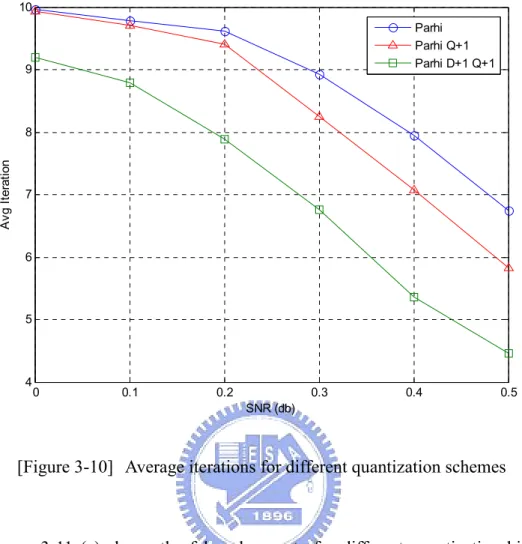
【Figure 3-10】】】】 Average iterations for different quantization schemes 34 【

【 【

【Figure 3-11】】】】 False alarm rate for different quantization schemes 36 【

【 【

【Figure 3-12】】】】 Turbo decoder decoding flow with give-up and state re-use scheme (give-up detection before termination checking) 38 【

【 【

【Figure 3-13】】】】 Turbo decoder decoding flow with give-up and state re-use scheme (give-up detection after termination checking) 39

【 【 【

【Figure 3-14】】】】 The false alarm rate of different decoding flow 42 【

【 【

【Figure 3-15】】】】 Traditional turbo decoding flow with termination scheme 44 【

【 【

【Figure 3-16】】】】 Average iterations for 1000 valid packets 46 【

【 【

【Figure 4-1】】】】 The Gamma calculation unit 48 【

【 【

【Figure 4-2】】】】 Block diagram of ACSO unit 49 【

【 【

【Figure 4-3】】】】 The forward processor unit with memory (FP) 49 【

【 【

【Figure 4-4】】】】 The soft-output calculation unit 50 【

【 【

【Figure 4-5】】】】 The row-by-row scheme for data writing 51 【

【 【

【Figure 4-6】】】】 Data arrangement after intra-row permutation 52 【

【 【

【Figure 4-7】】】】 Data arrangement after inter-row permutation 52 【

【 【

【Figure 4-8】】】】 The column-by-column scheme for data reading 53 【

【 【

【Figure 4-9】】】】 Space and time relationship for α-first memory

management 55

【 【 【

【Figure 4-10】】】】 Block diagram for SW log-MAP decoder 55 【

【 【

【Figure 4-11】】】】 The PE controller 57

【 【 【

【Figure 4-12】】】】 Block diagram of give-up detection circuit 58 【

【 【

【Figure 4-13】】】】 Artisan’s memory compiler 59 【

【 【

【Figure 4-14】】】】 MAP chip layout by SoC Encounter 61 【

【 【

【Figure 6-1】】】】 State diagram for Type-I and Type-II HARQ Protocol

List of Tables

【 【 【

【Table 2-1】】】】 Information block lengths and rates 18 【

【 【

【Table 3-1】】】】 Different quantization scheme for MAP 31 【

【 【

【Table 3-2】】】】 Iteration reductions and throughput increase for

different channel SNR 46

【 【 【

【Table 4-1】】】】 Area report for each component 59 【

【 【

Chapter 1 Introduction

With the performance approaching the Shannon limit of channel capacity, turbo codes [1] [2] represents one of the most popular research topics in coding theory and have been deployed in many designs of communication systems such as wireless systems. Although turbo code provides powerful ability for error control coding, it also requires a lot of power consumption during the iterative decoding process. Thus, low-power turbo decoder design becomes an important research issue for communication systems operated with stand-alone batteries. Due to the iterative decoding style of turbo code, to reduce unnecessary iterations means to save the energy consumption and has been studied in many references [12] [18] [27]. This kind of techniques is called early-termination while decoded outputs are already correct patterns.

When the channel condition becomes noisy, the decoded output is possibly unreliable even as maximal iteration number is reached. In [20], a neural network training method is proposed to estimate the patterns of decoding errors for re-transmission. Similar to the idea in [20], we find out a possible pattern of decoding error through simulations and we propose early give-up technique to stop the decoding process in advance. Then a request of re-transmission is sent. A reuse method is also proposed to utilize the prior MAP information of the given-up process as the initial condition for next transmission, based on the correlation between the same packets transmitted at different times. The early give-up algorithm is acquired from observations of simulation results, so there exists possible mis-judges, i.e. false alarms. Under poor channel conditions, the simulations show that both the average iteration number of turbo decoding process and the overall decoding latency are

reduced despite of the existence of false alarms.

1.1 Motivation

For battery-based applications like cell-phone or other portable devices, power issues get more and more concerns recently. Our main job is to design a turbo decoder which can use energy more efficiently depends on the channel conditions. With no unnecessary energy waste for decoding, we can increase the use time for battery-based applications with turbo coding and also increase the life time for the battery.

1.2 The Proposed Scheme

The turbo decoding is a kind of iterative decoding process. For power saving aspects, a lot of papers discuss how to save unnecessary iterations for the situation that the decoded outputs are already correct decoded pattern during decoding process. This kind of techniques called termination skills [4] [18]. In this situation, because the channel condition is good enough, a few iterations will be able to decode out the correct patterns so we can stop decoding process before reach the preset limit (maximum iteration).

However, in this thesis, we think about the other side of situation that if channel condition goes very bad (over the decoding ability of the turbo decoder), whether we should stop decoding process preventing unnecessary iterations for power saving?

According to our motivations, we propose a new idea called “Early Give-up” which can detect the channel condition during decoding process by decoded extrinsic

stage are reliable (error free) or not. If the estimation shows that we will get the unreliable decoded pattern finally, the decoding process will be stopped for energy saving, and request for re-transmission immediately to reduce overall decoding latency.

Besides that, we also present a methodology for re-use the work we calculated before the give-up stage. According to the simulation results, we prove that we can reduce the overall average decoding iterations for given valid packet numbers under bad channel conditions by using “Early Give-up” with reuse state methodology, thus we can save power and reduce decoding latency under bad channel conditions.

1.3 The Arrangement for Thesis Chapters

This Thesis is structured as follows. Chapter 1: Introduction

Chapter 2: Turbo Coding Technology

In this chapter, we will briefly explain the encoding and decoding algorithm for turbo code and corresponding hardware structures. Besides, we also take implementation issues into considerations, like log-MAP algorithm, fixed-point implementation effects, sliding window algorithm and some termination techniques for turbo decoding. In the end of this chapter, we will introduce turbo code as an application in the communication field.

Chapter 3: The Early Give-up and State Reuse Methodology for Turbo Coding In this chapter, we will explain our new idea “Early Give-up” technique for turbo decoding, and corresponding re-use methodology for re-send process. We will modify

the turbo code decoding flow with the new idea and show simulation results for the proposed scheme in this chapter.

Chapter 4: Hardware Implementation

In this chapter, we will explain each component in turbo decoder for realizing MAP algorithm, and also introduce the Early Give-up detection circuit for implementation. We will compare the overhead from area and power point of view in the end of this chapter to judge the new idea’s contributions.

Chapter 5: Comparison and Conclusion

We will compare the benefits and overheads for Early Give-up from hardware and power point of view and make conclusions for the thesis in this chapter.

Chapter 6: Future Works

In this chapter we will present the future works relative to our research in this thesis as the direction for future research topics.

Chapter 2

Turbo Coding Technology

What is Turbo Code

Turbo code was firstly introduced in 1993 by Berrou, Glavieux and Thitimajshima [1]. They promised almost 10 dB coding gain (at BER=10-5), which is within 0.7 dB of Shannon limit in AWGN channel. Special features of turbo code are as follows: (1) turbo code are composed of two parallel-concatenated recursive systematic convolutional code (RSC) with (usually) very long block length (2) A pseudo random interleaver is used to randomize the input data for second RSC encoder (3) The decoder uses iterative MAP algorithm. These factors combined make turbo code great abilities for error correcting, and also make turbo code a milestone in error control coding area.

2.1 The Encoding and Decoding Structure for Turbo Code

The encoder side for turbo code uses two the recursive systematic convolutional code (RSC) and one interleaver, as figure 2-1 shows. Code rate can be increased to 1/2 by puncturing (without puncturing, the code rate will be 1/3). The decoder parts are shown in figure 2-2. De-puncturing action for decoder is according to encoder. Other parts are composite of two SISO (Soft-Input Soft-Output) decoder、interleaver and de-interleaver. The main concept for decoding is to use first SISO decoder which made use of the received value from channel and a-priori information to calculate the extrinsic information, and then take the extrinsic information as the a-priori information to the second SISO decoder. Iterating the decoding process to decrease

the bit error rate from decoder (refer to [1] for detail). For SISO decoder, it can be implemented by MAP algorithm or Soft-output Viterbi algorithm (SOVA) [8].

[Figure 2-1] Turbo encoder system block diagram

e L₁₂

e

L₂₁

[Figure 2-2] Turbo decoder system block diagram

2.2 The MAP Algorithm

BCJR Algorithm (MAP) was firstly presented in 1974 by Bahl, Cocke, Jelinik and Raviv [2]. BCJR algorithm is optimal for estimating the states or the outputs of a Markov process observed in white noise. The details of the algorithm are available in [2] [5] [6] [9] [10], we briefly describe the main idea of the MAP algorithm. The Log

( )

_[

[

]

_]

r

|

0

x

Pr

r

|

1

x

Pr

ln

ˆ

k k

=

=

≡

Λ

x

k (2.1)

Where r is the received symbol form channel and xk is the information bit.

Considering the state transition in trellis structure, we can express Pr[Xk=1|r] as follows:

∑

+ ∈ = = = = S s) , (s k ' 1 -k k ' r) | s S , s Pr(S r] | 1 Pr[x (2.2)

Where S+ is the set of all pairs of states which transient from state s’ at time k-1 to state s at time k due to xk = 1. Similarly,

∑

− ∈ = = = = S s) , (s k ' 1 -k k ' r) | s S , s Pr(S r] | 0 Pr[x (2.3)

Where S- is the set of all pairs of states which transient from state s’ at time k-1 to state s at time k due to xk = 0.

Hence, the LLR of the kth input bit of the input sequence x is obtained as:

( )

₍

(

)

₎

          = = = = = = = = Λ

∑

∑

− + ∈ ∈ S s) , (s k ' 1 -k S s) , (s k ' 1 -k ' ' r) s, S , s Pr(S r) s, S , s Pr(S ln r 0 Pr r 1 Pr ln ˆ k k k x x x (2.4)

If Λ

( )

xˆ_k >0, we decode the input bit xk as 1, otherwise, the input bit as 0.

Take Pr(Sk-1=s’, Sk=s, r) into consideration, By using Bayes’ rule, we can partition the joint probability of Pr(Sk-1=s’, Sk=s, r) into three parts.

) Pr( ) , Pr( ) , Pr( ) , , Pr( ) , , Pr( 1 1 1 1 1 k n j k k k k k j k k k k k S r S S r r S r S S r s S s S ≤ < − < ≤ − − − = ≡ = ′ = (2.5)

Define the three probabilities as follows:

) , Pr( ) ( _{1 1 1} 1 k k j k k− S − ≡ S − r≤ < α (2.6) ) , Pr( ) , ( _{k−1 k} ≡ _{k k k−1} k S S r S S

γ

(2.7)

) Pr( ) ( _{k k j n k} k S ≡ r < ≤ S

β

(2.8)

Where αk-1(Sk-1) is the function of received information prior to the stage k, γk(Sk-1, Sk)

is the function of received information for stage k and βk(Sk) is the function of

received information after stage k. αk(Sk) can be computed recursively as:

∑

∈ − − − ≤ ≤ = ′ ′ ≡ S s k k k k k k j k k k S S r S S S ' 1 1 1 1 ) ( ) ( , ) , Pr( ) (

α

γ

α

(2.9)

where S is the set of trellis state transition. Similarly βk(Sk) can be computed

recursively as:

∑

∈ − − ≤ ≤ − − ≡ = ′ ′ S s k k k k k k n j k k k S r S S S S ' 1 1 1 1( ) Pr( )

β

( )

γ

( , )

β

(2.10)

The function

γ

_k(S_k−1,S_k)can be expressed as:

) ( ) ( ) ( ) , Pr( ₁ , k k k k k k k k m i k ≡ r S S − = p x =i p x′ x p p′ p

γ

(2.11)

Where i is the input bit that cause the transition from state Sk-1=s’ to Sk=s, and xk ` pk

are the systematic bit and parity bit respectively.

From equation (2.4)-(2.11), we can obtain the following equation:

( )

₍

(

)

₎

          = = = = Λ

∑∑

∑∑

− − − − − − − − k k k k S S k k k k k k S S k k k k k k k k k S S S S S S S S x x x 1 1 ) ( ) , ( ) ( ) ( ) , ( ) ( ln r 0 Pr r 1 Pr ln ˆ 1 0 1 1 1 1 1 1

β

γ

α

β

γ

α

(2.12)

m i k , γ ) ( ₁ 1 − − k k S α ₍ ˆ ₎ k X Λ β_k(S_k)

[Figure 2-3] MAP decoding flow chart

2.3 The Implementation Issues

From software point of view, BCJR algorithm will be fine for BER performance. But if it talks to hardware implementations, that will be lots of factors to effect the overall performance. Like the performance degradation due to fixed-point realization, and for real-time demands and decreasing memory area (saving power), take sliding window method for implementation, the effects for the performance. We also talk about some techniques for reducing unnecessary iterative process for termination. Therefore, the following sections will be from the hardware point of view to talk about the questions and solutions from papers.

2.3.1 The Log-MAP Algorithm

Though MAP decoding can achieve great error correcting capacity near Shannon limit, this algorithm is too difficult to be realized, basically because the numerical representation of probabilities, non-linear functions and mixed multiplications and additions of these values. For the SISO decoders, Log-MAP algorithm is suitable for

hardware implementation, due to its relative simplicity compared with original MAP algorithm, and better performance than SOVA [5].

The Log-MAP algorithm is a transformation of MAP, which has equivalent performance and without its problems in practical implementation. It works in logarithmic domain, where multiplication is converted to addition. From (2.9), we can define forward state metrics α in log domain.

) ln( ln ) , ( ) ( ln ) ( ln ) ( ' ) ( ) ,' ( ' ) ( ) ,' ( ' 1 1 1 1 1

∑

∑

∑

∈ + ∈ ∈ − − − − − =      _⋅ =       _{′ ′} = ≡ S s s s s S s s s s S s k k k k k k k k LM k LM k LM k LM k LM k _{e e} e S S S S S α γ α γ

γ

α

α

α

(2.13) Where

γ

_kLM(s',s)≡ln

γ

_k(s',s)

Form (2.10), we can derive backward state metric β in log domain.

) ln( ) ln( ) ( ln ) ( ' ) ' ( ) ,' ( ' ) ' ( ) ,' ( ' 1 1 ' 1 1

∑

∑

∈ + ∈ − − − − ≡ = ⋅ = S s s s s S s s s s k k k LM k LM k LM k LM k LM k _{e e} e S S

β

γ β γ β

β

(2.14)

Therefore, from (2.12) the log-likelihood ratio is given by

( )

        −         =           =           = Λ

∑∑

∑∑

∑∑

∑∑

∑∑

∑∑

− − − − − − − − − − − − − − − − − − − − − − − − + + + + + + + + k k k LM k k k LM k LM k k k k LM k k k LM k LM k k k k LM k k k LM k LM k k k k LM k k k LM k LM k k k k LM k k k LM k LM k k k k LM k k k LM k LM k S S S S S S S S S S S S S S S S S S S S S S S S S S S S S S S S S S S S k e e e e e e e e e e x 1 1 0 1 1 1 1 1 1 1 1 1 0 1 1 1 1 1 1 1 1 1 0 1 1 1 1 1 1 1 ) ( ) , ( ) ( ) ( ) , ( ) ( ) ( ) , ( ) ( ) ( ) , ( ) ( ) ( ) , ( ) ( ) ( ) , ( ) ( ln ln ln ln ˆ β γ α β γ α β γ α β γ α β γ α β γ α (2.15)

By use of equation: max*(x,y)≡ln(ex +ey)=max(x,y)+ln(1+e−x−y) (2.16)

We can get _kLM(s) max*

(

[

_uLM₀(s',s) _kLM₁(s')

] [

, _uLM₁(s',s) _kLM₁(s')

]

)

k k= + − = + − =

γ

α

γ

α

α

(2.17) from (2.13). _kLM₁(s) max*

(

[

_uLM₀(s',s) _kLM(s')

] [

, _uLM₁(s',s) _kLM(s')

]

)

k k

β

γ

β

γ

β

₋ = ₌ + ₌ + (2.18)

( )

ˆ max (

[

( ', ) ( ) ( ')

]

) max (

[

( ', ) ₁( ) ( ')

]

) ) ,' ( 0 * 1 ) ,' ( 1 * s s s s s s s s x _kLM _kLM _kLM s s u LM k LM k LM k s s u k k k β α γ β α γ + + − + + = Λ ₋ = − = (2.19)

2.3.2 The Fixed-point Effects

From hardware implementation and real-time demanded point of view, using fixed-point method to realize MAP algorithm is the best solution for cost and performance. So we will discuss the considerations of quantization on the performance proposed in [7] [16] [26].

In [16] [26], they consider the internal MAP state variables and channel data from A/D outputs then simulate the different quantization schemes for BER compared to infinite precision case to find the minimum precision representation under tolerable performance degradation. The meanings for minimum bit representations are not only for cost-down in hardware implementations but also for power saving due to minimum storage requirement and less switching activities.

Paper [7] talks about the size of look-up table for Log-MAP. The core of Log-MAP is the operation_Max*(_A,_B)=_Max(_A,_B)+ln(1+_e−|A−B|)=_Max(_A,_B)+∆_, according to the quantization scheme, the ∆ in above equation can be expressed

as ) 2 | | exp 1 ln( |)) | exp( 1 ln( p B A B A− ≅ + − − − + ≡

∆ , where p is number of precision

bits. We can find the minimum positive integer m stored in ROM satisfying the

inequality ln(1+exp(−m/2p))≤2−(p+1) to minimize the effects due to look-up table

2.3.3 The Metric Normalization

An important issue in Turbo Decoding fixed-point operation is the growing of state metrics over the finite numerical range representation. The same problem also can be found in Viterbi’s algorithm [22]. In 1999, Parhi had proposed a solution in [16]. This method requires small amount of hardware and its speed does not depend on the number of state. His approach is that if the word length of state metrics is q bits, once the state metrics is larger than 2q−2, then subtract 2q−2 from all state metric

)

(α or β . The proof is as follows:

The Max* operation is: Max*(x+z, y+z) = Max(x+z, y+z) + ln(1+e-|(x+z)-(y+z)|) (2.20)

Thus Max*(x+z, y+x) = Max(x, y) + z + ln(1+e-|x-y|) = Max*(x, y) + z (2.21)

According to equation (2.21), Max* operation is linear. Thus a global shift for α and β

in (2.17) (2.18) won’t change the value of L(uk) in (2.19) since the contribution of z,

when put outside two Max* operations, is cancelled [17].

2.3.4 The Sliding Window Method for Turbo Decoder

According to section 2.3.1 above, we have simplified the MAP decoding complexity by log-MAP equation. However, for log-MAP decoding algorithm, we

still have to store every branch metric (γ) and forward state metric (α) at every

stage until the backward state metrics (β) had been calculated out, so as to compute

LLR in (2.19)

Taking 3GPP specification for example, according to encoder structure, we have 8 states in trellis diagram, if we express every state by 8 bits, it would require 64 bits of storage per branch, and if the frame size is 1024 bits, the turbo decoder must at

least have 64x1024=64K bits storage for traditional MAP decoding algorithm.

Because lots of memory requirement and decoding latency for MAP decoding, Viterbi proposed sliding window [3] structure as a solution for these questions in 1998. We will briefly explain his idea by figure 2-4. First of all, we have three process elements for sliding window (SW) MAP decoding algorithm, one for forward processing and the other two for backward processing. L means the sliding window length (typically 6-10 times for constraint length). The label for each node below means the trellis time instance. The main idea for sliding window method is that we can estimate real backward state metric condition by applying learning period (L). As figure 2-4 shows, dash line means that the unreliable backward branch metric computations (learning period). After learning period, we get reliable initial state condition for backward state metrics computations. Now we take first decoded output for example to explain how these three process elements function. We compute forward state metrics as the label shows. From time 2L to 3L, we compute the node metric from 0 to L, at the same time (2L-3L), the first backward processor start to learning the backward state by received data from 2L to L. During learning period, we do not store anything until time goes to 3L, at this time instance (3L), because the forward processor had been already computed the forward state metric from 0 to L, so we can combine the forward and backward state metrics to get valid decoded output (L to 0) from time 3L to 4L.

The operation for second backward processor will be same as the first backward processor. While the first backward processor decode out branch from L to 0 at time 3L to 4L, second backward processor will start learning at time 3L. After learning period, we can get decoded output for branch 2L to L from second backward processor from time 4L to 5L. Two backward processors will take turn to decode out the branch as the timing in figure 2-4 shows. This is the way for sliding window MAP

algorithm functions.

[Figure 2-4] Timing diagram for sliding window method (refer to [3])

2.3.5 The Termination Techniques for Turbo Code

Termination is a kind of power saving technique for turbo code. Traditional way for stopping of turbo decoding is to set a maximum iteration limit and whether decoded outputs are valid or not, decoding iteration will not stop until the preset limit. This is not a smart way for iterative decoding process, so lots of papers talk about when to stop properly, this kind of technique calls termination.

The termination techniques can be split into two categories, one is made use of inner forces and the other is made use of external forces [4]. Observing convergence for decoding data with the number of iterative process increased to decide whether continue decoding or not calls the inner force method. The other way calls external force, it means to use another kind of error control coding prior to turbo encoder to

illustrated in figure 2-5 (taking CRC as outer code for example). My thesis uses CRC as the outer code for termination scheme.

(a) Turbo-CRC encoder

e

L₁₂ e

L21

(b) Turbo-CRC decoder

[Figure 2-5] Turbo-CRC encoding and decoding block diagram

2.4 Applications for Turbo Code

In this section we will briefly describe two applications of turbo code in communication field, and corresponding specifications.

2.4.1 Application for 3GPP

First of all, we describe the encoder structure for 3GPP. As in Figure 2-6, Encoder’s part is made up of two convolution encoders, and for each encoder, the

generator matrix: ] ) ( ) ( , 1 [ ) ( 2 1 D g D g D G = , where g1(D)=1+D+D3, g2(D)=1+D2+D3. The

frame size for 3GPP specified is from 40 to 5114 bits per frame, and the code rate is 1/3. (In 3GPP2, the standard use two rate 1/3 constituent codes, both with generator

matrix ] 1 1 , 1 1 , 1 [ ) ( 3 2 3 2 3 2 3 D D D D D D D D D D G + + + + + + + + +

= , with rate from 1/5 up to 1/2). The

internal interleaver is implemented as an array with 5, 10, or 20 rows and between 8 and 256 columns, depending on the frame size K. Data is wrote in row-wise, intra-row and inter-row permutation is performed on the array. We will give a more detail example in chapter 4. The dash line in figure 2-6 is for termination to all-zero state.

[Figure 2-6] The Structure of turbo encoder (refer to [15])

The performance of 3GPP turbo decoder is in figure 2-7 [6]. Simulation is implemented on TI DSP using Max-Log MAP algorithm. We can see the relationship

iterations.

[Figure 2-7] The performance of turbo decoder (excerpted from [6])

2.4.2 Application for CCSDS

CCSDS (Consultative Committee for Space Data Systems) takes turbo code in

channel coding standard recently. The additional coding gain of 2.5 dB at BER = 10-5

can be achieved by rate 1/6 turbo code with respect to the old standard. The encoder has two code rate 1/4, 16 states convolutional codes with generators

] 1 1 , 1 1 , 1 1 , 1 [ ) ( _{3 4} 4 3 2 4 3 4 2 4 3 4 3 D D D D D D D D D D D D D D D D G + + + + + + + + + + + + + + + = [23]. The

corresponding information rate and encoder structure are shown in table 2-1 and figure 2-8. For encoder, the information block buffer contains interleaver which is described in new CCSDS standard.

Code block length n Information length k

Rate 1/2 Rate 1/3 Rate 1/4 Rate 1/6

1784 3576 5364 7152 10728

3568 7144 10716 14288 21432

7136 14280 21420 28560 42840

8920 17848 26772 35696 53544

16384 32776 49164 65552 98328

[Table 2-1] Information block lengths and rates

Chapter 3 Early Give-up and State Reuse

Methodology for Turbo Coding

3.1 Motivation

According to simulations of paper [4] [18], when channel condition goes very bad (SNR very low), the decoding iterations needed will be very close to maximum iteration during decoding process (shown in figure 3-1). Sometimes after final iteration for decoding, we still get wrong information from decoder output (decoded failure frame). This result points that when messages are interfered by noise seriously, it may be not a smart way to continue decoding process (because lots of time we may get decoded failure frame in the end). So we present a technique calls Early Give-up. The so called “Early Give-up” means that during decoding process, once we find the trend of decoding failed, we will stop the decoding procedure immediately not until to maximum iteration! The goal of early give-up is to prevent power consumptions for unnecessary iterations.

Giving up decoding process is not enough to decode a valid frame out, it needs re-send frame to complete decoding process (As for a decoding frame at maximum iteration but failed finally, it also needs re-send scheme, so “Early Give-up” gets benefits from (1) no waste iterations for power saving (2) early re-send to shorten overall decoding latency). According to above reasons, we can improve the QoS (Quality of Service).

Besides, we have a reuse scheme for give-up. Reuse means that we can save the previous work during give-up and use it for re-send the same packet as initial conditions. We prove it by simulation. Reuse state methodology really can reduce

overall average decoding iteration numbers for successful decoded frames.

[Figure 3-1] Simulation result for SNR vs. average iteration (excerpted from [18])

3.2 Observation and Simulation for Early Give-up

Observing failure frame’s properties during simulation, we find the common feature of decoding failed frame is that the extrinsic information of most decoding failed frame will be oscillating with decoding iterations increasing. The oscillation means that the average absolute value of extrinsic information will not increase monotonically with decoding iterations increasing [12] [30]. In other words, if it can’t gain additional information (judged by average absolute value of extrinsic information) from iterative decoding process, more iteration may be useless!

3.2.1 The Trends of Extrinsic Information

through iterations, turbo decoding decrease the variance σ2, so

∑

= = N k k i m L L u N M 1 ) ( | | | ( )| 1 increase. (Q Y u Y f u Y f Y u Y u x L m k k e k k e 2 2 ) 1 ( ) 1 ( log ) 1 Pr( ) 1 Pr( log ) (

σ

= − = + = = − = + = = ,

[

L x

]

E

[ ]

Y E m 2 2 ) ( σ = , so

σ

_m ↓thenM_|L| ↓)

[Figure 3-2] |LLR| trends for different types of decoding packets (excerpted from [12])

According to the idea and error pattern of [12], we also analyze the data during decoding process. The sample data for extrinsic information from decoding process as in figure 3-2, we can find the property that, for most decoding failed frame (in red color marked by ‘x’), the mean of absolute value of extrinsic information (Le) will not increase with iteration stepping up (oscillation for Le). Thus, we made a rule (Early Give-up) that when we get the information of oscillation for average absolute value of extrinsic information during decoding process, from the experience of successful decoding point of view, we should give-up the decoding process immediately for power saving. Therefore, we use the oscillation of extrinsic information as the criteria for give-up detection.

0 2 4 6 8 10 12 14 16 18 20 0 2 4 6 8 10 12 14 16 18 Iterations M e a n o f |L e | x failure frame + error free frame

0 2 4 6 8 10 12 14 16 18 20 0 2 4 6 8 10 Frame size = 512 Number of Iteraions M e a n o f |L e | 0 2 4 6 8 10 12 14 16 18 20 0 2 4 6 8 10 Frame size = 256 Number of Iteraions M e a n o f |L e |

[Figure 3-4] The trends of extrinsic information for different frame size

In figure 3-3, the simulation results are for frame size=1024 bits, we also observe different frame sizes for oscillation phenomena, as figure 3-4 shows. From the experiment results, we concluded that the estimation of decoding failed case is more reliable as the frame size increased. The reason is, for longer frame size, we have more side information about the bit we estimated, so the decoding failed case estimated by oscillating can be more accurate.

3.2.2 Simulation Results for Give-up

According to our idea, we simulate the give-up effects for decoding performance judged by packet error rate. Note that, in this case, we just give simulation results for give-up only. However, give-up is not enough for decoding a valid packet out, so we

will discuss the give-up effects in section 3.5 for the system with re-transmission scheme, and then give a complete conclusion there.

0 0.05 0.1 0.15 0.2 0.25 0.3 0.35 0.4 0.45 0.5 10-2

10-1 100

Simulation for Give-up effects

SNR (dB) P a c k e t E rr o r R a te Optimum Early Give-up 0 0.05 0.1 0.15 0.2 0.25 0.3 0.35 0.4 0.45 0.5 2 4 6 8 10 12 14 16 SNR (dB) A v e ra g e I te ra ti o n Optimum Early Give-up

[Figure 3-5] Effects on the performance by give-up decoding process

In figure 3-5, we set the number of maximum iterations to be 15, and the optimal means that the program compared the information bits in encoder and decoded outputs after per iteration of decoding process. If the output of encoder and decoder are the same, we stop the process immediately for saving unnecessary iterations (This is impossible in practical, because we don’t know what exactly the information bits for encoder, so this method is only available in simulation, therefore, paper [27] called it’s an optimal (or Magic Genie Rule) solution).

valid, we should use the termination techniques mentioned in chapter 2. Besides, we analyze the performance by packet error rate (PER), rather than bit error rate (BER), that because once we found a decoded failed packet, no matter one bit error or one hundred bit errors in it, we all need re-transmission, so from system level point of view, PER (or frame error rate, FER) is more meaningful than BER.

3.3 The Reuse Methodology for Early Give-up Scheme

By using the early give-up technique, the turbo decoding process can be stopped as early as possible while the channel condition is not good enough. The simulations show that energy can be saved even with the presence of false alarms. Another question is that if there exists useful information within the given-up process except for energy savings. Turbo decoding is an iterative process and requires the initial guess. We assume that there exists certain correlation between the same packets transmitted at different times. Therefore, a reuse method is proposed to utilize the calculated information of the given-up process and use it as the initial guess for re-transmitted packet. So section 3.3.1 will describe the re-use method detaily and the corresponding assumption conditions. Section 3.3.2 will show the simulation results for reuse methodology.

3.3.1 The Idea of Reuse Methodology

.

Traditionally, the initial condition for MAP decoding algorithms is set to be 0 based on the assumption that the probability of information bits to be 0 or 1 is

0 1 log 5 . 0 5 . 0 log ) 0 Pr( ) 1 Pr( log = = = = = n n k k n u u

. By applying the re-use technique, we save the extrinsic information calculated in the previous given-up process and use it as the initial condition of MAP decoding for the re-transmitted packet based on the correlation between the same packets transmitted at different times. The circled part in figure 3-6 shows the reuse part for explanation. Instead of starting from 0 as initial condition, we utilize the prior estimated values of information bits as initial guess. This will lead to the iterations reduction of decoding processes and we will give the simulation results in section 3.3.2.

) ' (x α

xˆ

) ( (2) 1 e L − α ' 1 p ' x ' 2 p ) 1 ( Λ ) 2 ( e L ) 2 ( Λ ) ( (1) e L α

[Figure 3-6] The reuse methodology for turbo decoder

3.3.2

The Simulation Results for State Reuse Methodology

The simulation results in figure 3-7, figure 3-8 demonstrate the average iteration numbers of decoding processes with the reuse state technique. The X-axis represents the SNR offset. The SNR offset means the SNR difference between the given-up packet and the re-transmission packet. To be conservative, we assume that the channel SNR becomes better than the previous given-up transmission, so that the resent packet

will have better chance to be correctly decoded. Therefore, the SNR offsets mean the difference between two transmissions of the same packet.

The original channel SNR of two simulation cases are shown in figure 3-7 and figure 3-8. Figure 3-7 is the case that the original channel SNR to be 0.0 dB and figure 3-8 is the case that the original channel SNR to be 0.5 dB. The SNR of the resend packet is according to the SNR offset. For example, if the original channel SNR is 0.5 dB (the case in figure 3-8) and the offset is 1.0 dB, the channel SNR of the re-transmitted packet is assumed to be 1.5 dB. Therefore, if the SNR offset is 0, it means that both transmissions are under the same channel condition.

The SNR offsets in the simulations are all positive because the early give-up/reuse state techniques proposed in this study focus on the worse channel conditions. If the re-transmitted packet bears worse channel SNR than the given-up packet, the possibility to decode correctly is much less.

Here are the specifications and simulation results. [Reuse Experiment 1]

Specifications:

Frame size = 1024 bits

Maximum iteration = 10 times

SNR (for the given-up packet) = 0.0 dB Total Early Give-up times = 200 times

0 0.5 1 1.5 1 2 3 4 5 6 7 8 9 10

Simulation for Reuse Method at 0.0 dB

SNR offset A v e ra g e i te ra ti o n WithRM WithoutRM

[Figure 3-7] Reuse method for SNR at 0.0 dB

[Reuse Experiment 2]

Specifications:

Frame size = 1024 bits

Maximum iteration = 10 times

SNR (for the given-up packet) = 0.5 dB Total Early Give-up times = 200 times

0 0.5 1 1.5 1 1.5 2 2.5 3 3.5 4 4.5 5 5.5 6

Simulation for Reuse Method at 0.5 dB

SNR offset A v e ra g e i te ra ti o n WithRM WithoutRM

[Figure 3-8] Reuse method for SNR at 0.5 dB

The green line (marked by diamond) is the result for the traditional case (taking 0 as initial condition for the re-send packet) and the blue line (marked by square) is the result for the re-use case (taking the extrinsic information at given-up stage as initial condition for the re-send packet). The goal of the reuse experiments is to prove that the decoding process will be converged faster if we use the information estimated at the given-up stage as the initial condition instead of traditional initial condition (0). Therefore, the experiment will focus on the decoding iterations of the re-send process.

The stopping condition for this experiment is to reach the pre-set number (total early give-up times in the specification: 200 times) of the re-send process. The figure 3-7 and figure 3-8 are plotted according to the average decoding iterations under 200 times of the re-send process for both traditional flow and re-use methodology. The number of the total transmission packets in this experiment must more than 200 packets, because not every transmission will request the re-transmission and we count

the re-transmission process only. Taking figure 3-8 for example, under the assumption conditions, we can reduce average decoding iteration about 1.8 iteration at the SNR offset 0.5 dB by re-use methodology compared to the traditional flow and thus, we can use less energy (proportional to the number of decoding iterations) for decoding a valid packet out with re-transmission.

From the simulation of above two case, we can give the conclusion: The reuse method for early give-up procedure is more usable for the case that the packet is given-up under better channel SNR, because the extrinsic information in better channel condition are more reliable than in bad channel, so the estimation will be more accurate and useful for decoding process.

3.4 The False Alarm for Early Give-up Technique

The give-up idea we proposed is that once the packet is estimated be a failed case, we give up decoding process as early as we could for power saving and hence, reducing latency for re-transmission. However, the give-up is a kind of estimation and we can’t estimate exactly accurate, therefore false alarm arises when the rest of iterations (if give-up not performed) can decode the valid packet out. In other words, if the alarm signs on the valid packet, it is the false alarm.

3.4.1 The Quantization Effects for False Alarm

The false alarm will be affected by a lot of factors like the size of the packets, the channel SNR and the decoding flow ...etc. In this section, we will combine these effects above to discuss the false alarm. We will simulate different quantization

conclusion from simulation results.

First, we want to explain the meaning of the symbol we used for quantization in Table 3-1. Taking Received value: q(4,2) for example, q is the abbreviation for quantization, 4 is the total bit numbers we represent the received value, and 2 is the precision bit numbers for received value. Thus, the received value is represented by 2 bits for dynamic range and 2 bits for precision bits (behind the dot). The column “Parhi” is the quantization scheme in his paper [16], and column “+Q1” means we add one precision bit compared with Parhi’s data. The column “+Q1+D1” means we add one bit for precision and one bit for dynamic range compared with Parhi. Table 3-1 shows the variables we used in MAP decoding process with different quantization schemes. Parhi [16] +Q1 +D1+Q1 +Q2 Received value q(4,2) q(5,3) q(6,3) q(6,4) Branch metric q(7,2) q(8,3) q(9,3) q(9,4) LLR q(10,2) q(11,3) q(12,3) q(12,4) Forward metric q(9,2) q(10,3) q(11,3) q(11,4) Backward metric q(9,2) q(10,3) q(11,3) q(11,4) Priori information q(6,2) Q(7,3) q(8,3) q(8,4) Extrinsic information q(6,2) Q(7,3) q(8,3) q(8,4)

[Table 3-1] Different quantization scheme for MAP

The simulation results for BER performance and average decoding iterations under different quantization scheme are shown in figure 3-9 and figure 3-10. (Figure 3-9 (a) and (b) are both simulation for BER but different in SNR range) We can see

from the simulation results that under terrible channel SNR (less than 0.5 dB), less precision quantization scheme will cause higher bit error rate and more iterations needed for decoding. Taking SNR=0.3 dB for example, the BER for Parhi’s

quantization is about 10-1 and is about 4x10-2 for Parhi+D1+Q1’s quantization scheme.

However, the number of average decoding iteration needed for Parhi’s quantization is about 9 times and is about 6.8 times for Parhi+D1+Q1 shown in figure 3-10. Therefore, in terrible channel SNR (< 0.5dB), using less precision quantization scheme will cause higher bit error rate and need more iterations for decoding due to the effects of quantization noise.

[Figure 3-9 (a)] BER for different quantization schemes

[Figure 3-9 (b)] BER for different quantization schemes

0 0.1 0.2 0.3 0.4 0.5 0.6 0.7 0.8 0.9 1 10-4 10-3 10-2 10-1 100 SNR B E R Parhi Parhi +Q1 Parhi +D1 +Q1 0 0.1 0.2 0.3 0.4 0.5 10-3 10-2 10-1 100 SNR (db) B E R Parhi Parhi Q+1 Parhi D+1 Q+1

[Figure 3-10] Average iterations for different quantization schemes

Figure 3-11 (a) shows the false alarm rate for different quantization bits. The false alarm rate is calculated according to the ratio of false alarm times and total alarm times (The total alarm times is illustrated in figure 3-11 (b)). The definition of the false alarm has been mentioned in section 3.4, here we explain the method we simulate. Because we do not know this alarm is true or false until the maximum iteration, therefore, we record this alarm and do not give-up until the maximum iteration for the false alarm experiment. If the decoded patterns are not valid patterns after maximum iteration, then this alarm is true, else it is a false alarm. From the simulation results of figure 3-11 (a), we conclude that, for the same dynamic range representation, false alarm rate will be decreased as the precision bits increased. Taking Parhi, Parhi+Q1, Parhi+Q2 for example, the number of precision bit of

0 0.1 0.2 0.3 0.4 0.5 4 5 6 7 8 9 10 SNR (db) A v g I te ra ti o n Parhi Parhi Q+1 Parhi D+1 Q+1

the false alarm of Parhi, Parhi+Q1, Parhi+Q2 are 3.5%, 1% and 0.2 %, respectively. That is because when we use more bits on precision, we will have less chance to mis-judge the oscillation case due to quantization. However, if we increase the representation for dynamic ranges, the quantization scheme will be less sensitive to the false alarm criteria (observing figure 3-11 (b), the alarm times of the Parhi+D1+Q1 are much less than the others). The experiment results for corresponding alarm times are shown in figure 3-11 (b). According to this experiment, we will choose the worst case of false alarm (Parhi+Q1+D1) as the quantization scheme to discuss the benefits of the proposed flow compared to traditional flow.

0 0.05 0.1 0.15 0.2 0.25 0.3 0.35 0.4 0.45 0.5 0 5 10 15 20 25 30 SNR (dB) F a ls e A la rm R a te i n p e rc e n t Parhi Parhi+Q1 Parhi+Q1+D1 Parhi+Q2 (a)

0

200

400

600

800

1000

1200

0

0.1 0.2 0.3 0.4 0.5

SNR (dB)

A

la

rm

t

im

es

Parhi

Parhi+Q1

Parhi+Q2

Parhi+D1+Q1

(b)

3.4.2 The Decoding Flow Effects for False Alarm

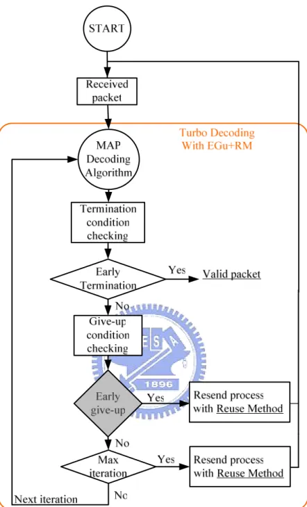
To achieve the goal of designing the energy efficient turbo decoder, we propose the scheme which is the combination of termination checking and give-up detection in decoding flow. However, how to decide the order of termination checking and give-up detection in the turbo decoding flow? To solve this problem, we simulate these two flows and the corresponding quantization effects of false alarm mentioned in above section, then we conclude by the simulation results of the false alarm to choose the best arrangement for termination checking and give-up detection as our proposed decoding scheme.

[Figure 3-12] Turbo decoder decoding flow with give-up and state re-use scheme (give-up detection before termination checking)

[Figure 3-13] Turbo decoder decoding flow with give-up and state re-use scheme (give-up detection after termination checking)

Figure 3-12 and figure 3-13 illustrate the different order of termination checking and give-up detection in decoding flow, and the corresponding false alarm simulation results are shown in figure 3-14. The decoding flow in figure 3-12 is stated: first, when receive a packet from channel, we use MAP algorithm to decode the packet.

After one iteration of the MAP decoding process, we will check the extrinsic information generated during the decoding process to see whether we are going to giving-up the decoding process or not. If the give-up checking shows that we should give-up the decoding process, we will request the re-transmission with re-use methodology. If the packet pass give-up checking, it will go to see whether it satisfy the termination condition. If the packet satisfies the termination checking, it is recognized as a valid packet under termination checking condition. If the packet does not pass the termination checking, it will check whether it reach the maximum iteration or not. If yes, the decoding process will request the re-transmission with re-use methodology, if no, the packet will go to next iteration of MAP decoding process. The difference between figure 3-12 and figure 3-13 is the order between give-up checking and termination checking, this is the point we want to decide by the simulation results of false alarm. Figure 3-14 (a) is the result for give-up detection first and the figure 3-14 (b) is the result for termination checking first. Comparing figure 3-14 (a) and figure 3-14 (b), we find that if we perform give-up detection before termination checking as in figure 3-12 shown, we will get higher false alarm in the higher (more than 0.4dB) channel SNR range. Taking SNR=0.5 dB for example, we will have false alarm rate about 13% with Parhi’s quantization scheme for give-up detection first flow (Fig. 3-12) and the false alarm about 7% for termination first flow (Fig. 3-13). That is because if we perform give-up detection first, we will mis-judge the case that the packet can pass the termination checking but been given-up before, and this case will be obvious in higher channel SNR of the simulation. Intuitively, the false alarm rate will go up as the channel SNR increased, that is because there will be more possible to decode a valid packet out under better channel SNR, to prevent the false alarm rate goes up severely for better (> 0.4dB) SNR range, we should use

therefore, we will take the decoding flow in figure 3-13 as our proposed decoding scheme.

0 0.05 0.1 0.15 0.2 0.25 0.3 0.35 0.4 0.45 0.5 0 5 10 15 20 25 30 SNR (dB) F a ls e A la rm R a te i n p e rc e n t Parhi Parhi+Q1 Parhi+Q1+D1 Parhi+Q2

(a) The early give-up before early termination in decoding flow (refer to fig. 3-12) 0 0.05 0.1 0.15 0.2 0.25 0.3 0.35 0.4 0.45 0.5 0 5 10 15 20 25 30 SNR (dB) F a ls e A la rm R a te i n p e rc e n t Parhi Parhi+Q1 Parhi+Q1+D1

(b) The early termination before early give-up in decoding flow (refer to fig. 3-13)

3.5 The Simulation Results of Proposed Scheme

Combining the factors we consider in above sections (including give-up detection, re-use methodology, quantization scheme, different decoding flow and the false alarm) we will give the simulation results including these factors to discuss the benefit of our proposed flow.

Firstly, we will compare the traditional flow and proposed flow then give the simulation results to explain the benefits of our scheme under the terrible channel conditions. As the figure 3-15 shows, the traditional flow for turbo coding system is illustrated. For traditional way, when received a packet, we decode the receive pattern by MAP algorithm. After per iteration of MAP decoding, we will check the opportunity for termination using some termination techniques mentioned in 2.3.4. If it is not the right time for termination, the process will check whether it reach the maximum iteration. If yes, it means that the decoding process reach max iteration but decoded output still not a valid pattern (because it failed to termination checking), so we will demand the transmitter to re-send the packet to complete data transmission. If no, we will continue the MAP decoding algorithm for next iteration.

[Figure 3-15] Traditional turbo decoding flow with termination scheme

The above flow is the same for turbo decoding with termination skill proposed in [12]. Now we will introduce our proposed flow for turbo decoding with proposed early give-up and re-use methodology. The flow is illustrated in figure 3-13. The differences between traditional flow and proposed flow are the give-up detection and reuse state methodology. In figure 3-13, according to the simulation result of false alarm, we add give-up decision after termination checking in decoding flow. After the termination checking, we will check the extrinsic information for termination checking to decide whether continue decoding process or not. If we decide to give up, we can re-use the state by the methodology mentioned in 3.3.1. The other parts are same to traditional flow.

To prove the give-up with reuse methodology really works for iteration reduction under bad channel condition, we made the following experiment. We set the

maximum iteration to be 10, and stop criteria is to receive 1000 valid packets at receiver for each SNR condition. The quantization scheme is the worst case for false alarm (Parhi+Q1+D1). Each packet contains 1024 information bits and the valid packet means that receiver decodes out a duplicate compared to the transceiver's message. By accumulating the number of decoding iterations, we can calculate the average decoding iterations for each valid packet.

The simulation assumptions are stated. Because we take re-transmission into consideration, there will be two kinds of cases for channel SNR. One is SNR for the give-up stage, and the other is for re-transmission stage. We assume the re-transmission packet will have 1 dB SNR offset better than the packet at give-up stage, for both traditional flow and our proposed flow. That is, if the packet with the SNR=0.4 dB at the give-up stage, then the re-transmission packet will have SNR=1.4 dB. The goal of this simulation is to prove that when the packet affected by noise seriously, stop decoding will be smarter than continue decoding process.

Under above assumptions and the simulation results, we can conclude from figure 3-16 that the idea we proposed really reduces iterations for decoding under terrible channel conditions. Taking SNR=0.4 dB for example, the traditional flow needs average 5.575 decoding iterations to decode a valid packet out and our proposed flow needs about 4.77 decoding iterations. Therefore, we can use less energy (according to iteration) to decode a packet out under our simulation conditions. The corresponding reduction percentages are in table 3-2.

From the throughput point of view, because the proposed scheme can use less decoding iterations for a valid packet under our assumptions, therefore, for given data to be transmitted, our flow can use less decoding iterations for the receiver compared to traditional flow, thus we can increase the through-put from iterations saving point of view. The corresponding increase in throughput compared to the traditional flow is

also reported in table 3-2. 0 0.1 0.2 0.3 0.4 0.5 0.6 0.7 0.8 2 3 4 5 6 7 8 9 10 11 12 SNR (dB) A v e ra g e i te ra to n s f o r p e r v a lid p a c k e t WithEGu+RM WithoutEGu+RM

[Figure 3-16] Average iterations for 1000 valid packets

SNR (dB) Average Iterations 0.0 0.2 0.4 0.6 0.8 Traditional flow 11.432 8.891 5.575 3.729 2.490 Proposed flow 7.108 6.369 4.770 3.323 2.435 Energy Saving 36.99 % 28.37 % 14.44 % 10.89 % 2.21 %

The increase for throughput (compared to traditional flow) 1.608 times 1.396 times 1.169 times 1.122 times 1.026 times

Chapter 4

Hardware Implementation

We have briefly described the encoder and the decoder structure for 3GPP system in chapter 2. The encoder part is easier than the decoder part for 3GPP, so the following sections will focus on the decoder for implementation. We take hardware architecture mentioned in [13] as the implementation blueprint to realize MAP algorithm and add the additional hardware for early give-up detection circuit. We will also estimate the overhead and the benefits for give-up from the point of area, power consumption and power saving.

4.1 A Case Study: The Turbo Decoder for 3GPP system

According to the idea we proposed in chapter 3, we take 3GPP standard as a case study to discuss the overhead of give-up, then compare the simulation results presented in chapter 3, to discuss the benefits of our idea. Therefore, the following sections will focus on the hardware implementation of process element, control unit and memory organizations.

4.1.1

The Process Element Design

As mentioned before in chapter 2, we have briefly described the MAP algorithm. So the goal of this section is to realize the process element including branch metric calculation, state metric calculation and soft-output calculation used in MAP algorithm.

4.1.1.1 The Branch Metrics (gamma)

The Branch metrics are calculated according to the formula below:

[

( ) ( )

]

2 1 ) , ( ) , ' ( _{k s,k p,k k s,k c s,k s,k p,k p,k} k s s =BM x x = L d ⋅x +L y ⋅x + y ⋅x γ , where L(dk)

and Lc are the a-prior information and channel reliability, respectively. The channel

reliability (Lc) can be implemented by look-up table according to real channel SNR

case. Some papers talked about the performance degradation affected by SNR mismatch [25]. However, in this thesis, we don’t touch this topic and assume the channel SNR is estimated accurately.

According to the structure suggested for 3GPP, we need to update every state metric in the same time stamp, therefore, we have to calculate every branch metrics out for updating the state metric on the corresponding trellis diagram. However, some

branch metrics calculations can be simplified by mapping rules

likeBM_k(1,1)=−BM_k(−1,−1), BM_k(1,−1)=−BM_k(−1,1), due to encoder structure and BPSK modulation. The block diagram of branch metric (gamma) calculation is in figure 4-1.

4.1.1.2 The Forward/ Backward State Metrics (alpha, beta)

The forward state metrics αk can be calculated recursively according to the

formula: ( ) ln exp[ ( ') ( ', )] max _'*( ₁( ') ( ', ))

' 1 s s s s s s s _{s k k} s k k k α γ α γ α = +      ₊ =

∑

_{− −} .

Similar to the ACS unit used in Viterbi’s algorithm, the process element we used to update the state metric is ACSO (Add Compare Select and Offset), the offset is compensation part for max* operation and corresponding block diagram is in figure 4-2. ) ( 4 1 + − j k s α ) ( 1 j k− s α ) , ( _{j 4 2j} k s+ s γ ) , ( _{j 2 j} k s s γ ) ( _{2 j} k s α

[Figure 4-2] Block diagram of ACSO unit

According to the FSM formula above, we need previous stage’s value to update FSM. Therefore, it needs registers to hold the state value as shown in figure 4-3. Besides, The LLR calculations also need FSM, so we need memory to store the value for the length of sliding window of the branch history.

) (

0 s

α