微型喇叭運用於行動電話之分析與設計

全文

(1)國立交通大學機械工程研究所. 碩士論文微型喇叭運用於行動電話之分析與設計. Analysis and Design of Miniature Loudspeakers for Mobile Phones. 研究生: 廖哲緯. 指導教授: 白明憲. 中華民國九十三年六月.

(2) 微型喇叭運用於行動電話之分析與設計 Analysis and Design of Miniature Loudspeakers for Mobile Phones 學生 : 廖哲緯指導教授 : 白明憲. Student: Jerwoei Liaw Advisor: Mingsian Bai. 國立交通大學機械工程系碩士論文. A Thesis Submitted to Institute of Mechanical Engineering College of Engineering National Chiao Tung University in Partial Fulfillment of Requirements for the Degree of Master of Science in Mechanical Engineering June 2004 HsinChu, Taiwan, Republic of China.. 中華民國九十三年六月.

(3) 微型喇叭運用於行動電話之分析與設計學生：廖哲緯. 指導教授：白明憲. 國立交通大學機械工程學系. 摘要. 近年來遠端通訊工業的快速發展。手機與個人數位助理等通訊產品對於聲音品質的要求是重要的。運用在這些產品的揚聲器稱為微型喇叭。微型喇叭是由振膜、音圈與框架組合而成，而這些物體的大小、形狀與材料性質會對微型喇叭的聲學特性造成影響。在這篇的論文中，我們將經由實驗與模擬的結果來分析微型喇叭。並且使用機電聲類比電路去模擬微型喇叭裝置於行動電話的動態響應。而機電聲類比電路則是利用電路分析的概念。對於機電聲類比電路參數的計算，在這裡我們採用測試箱法與曲線逼近的方式來求得。在電聲學裡，管路通常被當作只有質量效應，而管路的自然共振效應卻被忽略。在這篇的論文裡，我們將運用不同的方法去模擬管路的共振效應。開孔式與被動輻射式的揚聲器音箱設計概念被運用於行動電話的音箱設計，以增強低音的效果。. i.

(4) Analysis and Design of Miniature Loudspeakers for Mobile Phones Student: Jerwoei Liaw. Advisor: Mingsain Bai Institute of Mechanical Engineering National Chiao-Tung University. Abstract. The telecommunication industry is growing rapidly.. The demand of sound. quality is important in these telecommunication products like mobile phone or PDA. Loudspeakers applied in these products are called miniature speaker.. Miniature. speakers consist of a diaphragm, voice-coil and frame whose shape, size and material properties dominate the acoustic characteristics of them. In the paper, miniature speakers are analyzed by the experiment and simulation results.. Electro-mechano-acoustic (EMA) analogous circuit is used to simulate the. dynamic response of miniature speakers placed in mobile phone.. Delta compliance. and curve fitting method is adopted to calculate the parameters of the EMA analogous circuits. In theory of electroacoustics, duct is modeled by acoustic mass, but the natural resonance frequency of duct is never considered.. In this paper, the lumped. parameter oscillator model is used to model the natural resonance frequency of duct. And another method to model the resonance of duct is mentioned. The method of vented-box and passive radiator design is applied to design the well enclosure for mobile phone and enhance the bass response. ii.

(5) 誌謝. 轉眼間，研究生生活就在充實的學習與師長的教誨下度過。在此我首先要感謝白明憲教授給予我正確的學術研究態度與方向，使我不至於在茫茫學海中迷失方向。並且感謝老師對學生的照顧與關心，使我能夠順利完成學業。在論文寫作方面，感謝呂宗熙老師、陳宗麟老師能夠在百忙之中撥冗閱讀，並提出寶貴的意見與指導，使本文更趨完善。在學業與研究的進修方面，感謝學長曾平順、歐昆應、陳榮亮、李志中、蘇富誠及林家鴻；同學曹登傑、董志偉、林振邦、白淦元；學弟曾文亮、周中權、林建良、以及何柏璋彼此間的協助與砥礪，使我的實驗能有所進展，課業有所精進，在生活上彼此的照應，使的我可以愉快的度過研究生生活，大家朝夕相處的點點滴滴，亦是值得細細回憶。我也感謝所有給我精神支持的人，謝謝各位的幫忙與鼓勵。最後我以此篇論文獻給我所摯愛的家人，謝謝你們的勉勵與無私的照顧使我可以安心於學業之上。要感謝的人太多，以上列名恐有遺漏，在此一併致上最深的謝意。.

(6) TABLE OF CONTENTS. 摘要………………………………………………………………………i ABSTRACT…………………………………………………………….ii TABLE OF CONTENTS………………………………………………iii LIST OF FIGURES………………….………………………………...iv LIST OF PARAMETERS..…………………………………………….x 0 Introduction…………………………………………………………...1 1 Theory and Method………………………………………………...…3 1.1 Electro-mechano-acoustical analogous circuit…………......….3 1.2 The method of parameter identification..............................…...6 1.3 Modeling Acoustical System...............................................…...10 2 Simulation and experiment of results………….………….………..22 2.1 Parameter identification of miniature speakers…………….22 2.2 Modeling of the miniature speaker in mobile phones……….26 3 Bass-enhanced design for the miniature speakers…………....……31 3.1 The vented-box design…………………..………………………31 3.2 The passive-radiator design………………………………..…...33 3.3 Simulation results………………………….……………………37 4 Conclusions…………………………………………………….…...38 References…………………………………………………………40 Appendix……………………………………………………………42. iii.

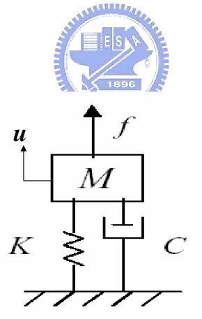
(7) List of Figures. Fig. 1.. Electro-mechano-acoustical analogous circuit of loudspeaker…………………………………………………....46. Fig. 2.. The mechanical system of loudspeaker. (M is diaphragm and voice coil mass, k is stiffness of suspension, C is damping factor)……………………………..…..…………..…46. Fig. 3. (a) An acoustic resistance consisting of a fine mesh screen (b) Analogous circuit of acoustic resistance……………...…...47 Fig. 4. (a) Closed volume of air that acts as an acoustic compliance (b) Analogous circuit of acoustic compliance………...…...….47 Fig. 5. (a) Cylindrical tube of air that behaves as an acoustic mass. (b) Analogous circuit of acoustic mass………..………..…….48 Fig. 6.. Analogous circuit for the radiation impedance on one side of a circular piston in an infinite baffle.....................................48. Fig. 7.. Geometry of the circular piston vibrating in a tube……………………………………………………….…...49. Fig. 8. Perforated sheet of thickness t having holes a of radius spaced a distance b on centers……….……………..……….49 Fig. 9. Fig. 10.. Geometry of the narrow slit………….………………......……50 Geometry of the duct (left side is entrance; right side is exit)……………………………………………..……………50. Fig. 11.. The curves of the tan(kl ) and the lumped method. (Solid line is tan(kl ) ; Dash line is lumped method)…………..…..…51. iv.

(8) Fig. 12.. Analogous circuit of lumped parameter oscillator model of a duct…………………………….………………...52. Fig. 13.. Equivalent circuit of a differential length ∆x of a two-conductor transmission line………………………..…...53. Fig. 14.. Equivalent circuit of a two-port model………….....….……..54. Fig. 15.. Impedance response comparison of simulation and experiment results for miniature speakers……………..…….55. Fig. 16.. The simple diagram of miniature speaker………………...….56. Fig. 17.. The real example of miniature speaker………………………56. Fig. 18.. The back side of miniature speaker………..…………………57. Fig. 19.. The front side of miniature speaker………………….……….57. Fig. 20.. The impedance response comparison of the three cases (Case 1: original speaker; Case 2: speaker without the damping material; Case 3: speaker without the damping material and the frame)…………………...........................................................58. Fig. 21.. The frequency response comparison of the three cases (Case 1 original speaker; Case 2: speaker without the damping material; Case 3: speaker without the damping material and the frame).......................................................................................59. Fig. 22.. The impedance response comparison of speaker and speaker with closed-port (closed-port means rear-side ventilation of speak is close)………...………………………….………..…60. Fig. 23.. The directivity of the Merry speaker (a) 500 Hz (b) 1k Hz (c) 2k Hz (d) 5k Hz (e) 7k Hz (f) 9k Hz (g) 10k Hz (h) 11k Hz ………..……………………………….…………………......61. v.

(9) Fig. 24.. The different views of enclosure for mobile phone……….........................................................................65. Fig. 25.. The analogous circuit of miniature speaker in mobile phone……………………………………..………………...65. Fig. 26.. (a) The structure of the front side of speaker (b) The analogous circuit of acoustic impedance Z AF ……………………………………………………...……..66. Fig. 27.. (a) The structure of the rear of the speaker (b) The analogous circuit of acoustic impedance Z AB …………………………………………………...………..67. Fig. 28.. The impedance response comparison of speaker and speaker in mobile phone……………...……………………..………68. Fig. 29.. The frequency response comparison of speaker and speaker in mobile phone……...….......……………….…….68. Fig. 30.. The impedance response comparison of experiment and simulation results………..……..…....…………………69. Fig. 31.. The frequency response comparison of experiment and simulation results…….…………..………….…………..….69. Fig. 32.. Electrical equivalent circuit diagram of low-leak of high-leak pinna simulator and IEC 711 Coupler. (Solid line: low-leak of high-leak pinna simulator; Dash line: 711 Coupler)…………................…..……….………....70. Fig. 33.. Simulation acoustic impedance for type 4195 Low-leak ear simulator compared to High-leak ear simulator …...........................................................................................70 vi.

(10) Fig. 34.. Simulation pressure frequency response for mobile phone coupled with low-leak and high leak Pinna……………….71. Fig. 35.. The simple diagram of the vented-box design………….…72. Fig. 36.. Low-frequency Model: EMA analogous circuit of vented-box system………………………………………...73. Fig. 37.. Low-frequency model: Acoustical analogous circuit of the vented-box system………………...……………….……...74. Fig. 38. The simple diagram of the passive radiator design…….……………………………...……………..….75 Fig. 39.. Low-frequency model: Acoustical analogous circuit of the passive radiator system………………..….………….……76. Fig. 40.. The frequency response comparison of Infinite Baffle and Closed-Box……………………...…………………….77. Fig. 41.. The simulation of impedance response of speaker and vented-box system……………………..….…………….…77. Fig. 42.. The simulation of the frequency response of vented-box system………………………..………………………….…78. Fig. 43.. The frequency response comparison of Infinite Baffle and vented-box system…………….………….…………….….78. Fig. 44.. The simulation of the frequency response of Passive radiator system…………………..……………………………….…79. Fig. 45.. The frequency response comparison of Infinite Baffle and passive radiator system…………………………...…….…79. Fig. 46.. The3-D diagram of the vented-box design for mobile phone………………………….………..……………….…80. vii.

(11) Fig. 47.. The frequency response comparison of Infinite Baffle and Vented-Box design……..………………………..……81. Fig. 48.. The frequency response comparison of Vented-Box: Vent open and Vent close……………..……….…….…….81. Fig. 49.. The 3-D diagram of the passive radiator design for the mobile phone………………...……….…………….….…..82. Fig. 50.. The frequency response comparison of Infinite Baffle and Passive Radiator design …………………….……..………………………..……...83. Fig. 51.. The frequency response comparison of Closed-Box and Passive Radiator design (Closed-Box means that passive diaphragm of passive radiator design is replaced and closed)…………………………………………….…...…..83. viii.

(12) List of Parameters Bl. = electro-mechanical transformation ratio, being product of magnetic flux density and voice-coil conductor length in air gap of loudspeaker driver. CA. = acoustic compliance of volume V. CM. = mechanical equivalent of C A. CMS = mechanical compliance of loudspeaker suspension system C AB = acoustic compliance of the air in the enclosure C AP = acoustic compliance of passive radiator suspension fs. = resonance frequency of loudspeaker driver. LE. = voice-coil inductance. QES. = electrical quality factor of loudspeaker. QMS. = mechanical quality factor of loudspeaker. QTS. = total Q of loudspeaker. M MD = mechanical mass of diaphragm M MS = mechanical mass of diaphragm and air-load M AP = acoustic mass of the air in the port or acoustic mass of passive radiator diaphragm. RE. = dc impedance of the loudspeaker. RAE = acoustical equivalent of R E ix.

(13) RMS = mechanical resistance of loudspeaker RAL = acoustic resistance of leak in box RAP = acoustic resistance of passive radiator SD. = effective area of diaphragm. ZA. = acoustic impedance. Z AB = acoustic impedance in the rear of diaphragm Z AF = acoustic impedance in the front of diaphragm ZVC = motional impedance. x.

(14) 0. Introduction Loudspeakers are important devices that are widely applied in many fields. The analysis technique of loudspeakers is well established. The history of loudspeaker is reviewed [1]. In this paper, Thiele and Small parameters will be used as the basis to analyze loudspeakers applied in mobile phone. Recently, consumer electronic products are rapidly developed. For the products of mobile phones and PDA, loudspeakers play an important role in these products. The loudspeakers applied in the product are usually called miniature speaker. These miniature speakers are widely used in many telecommunication products.. The. motivation for research of miniature speakers is that miniature speakers can have best sound quality when they are applied in mobile phone. [2], [3], [4] and [5] have well research in miniature speakers. These papers mainly focus on analysis of miniature speakers. In this paper, we not only analyze the miniature speakers but also discuss the enclosure design for miniature speakers. The analysis of method is Electro-mechano-acoustical (EMA) analogous circuit and lumped-parameter method. When the dimension of the system is smaller than the wavelength, the properties of loudspeaker such as mass and stiffness can be lumped to electrical elements such as inductance and capacitance. When miniature speakers are placed in mobile phones, the structure of mobile phone is complex and complex structure of mobile phone can be lumped to electrical elements. By the circuit analysis, the dynamic response of miniature speaker can easily be determined. For the mobile phone and PDA, their dimension is small. Thus the dynamic response for miniature speaker placed in mobile phone can be analyzed by lumped-parameter method.. When miniature speakers were placed in mobile phone,. 1.

(15) the structure of mobile phone may be influence the dynamic behavior of miniature speaker. The structure of mobile phone can be viewed as the acoustical impedance that causes some effects on the performance of miniature speaker. The acoustical impedance of structure can be lumped to acoustic mass, acoustic compliance and acoustic resistance.. In the theory of electroacoustics, acoustic mass, acoustic. compliance and acoustic resistance can be represented by inductance, capacitance and resistance. Thus we could mainly focus on acoustical system in EMA circuit and lump the acoustical impedance of structure to electrical elements. By using the circuit analysis, the dynamic response of miniature speaker placed in mobile phone is easily simulated. For enhancing the bass response of loudspeakers, the vented-box and passive radiator methods are the most popular methods and widely used in multimedia application. From the concept of vented-box and passive radiator method, this paper will use two methods to develop the suitable enclosure for the miniature speaker applied in mobile phone.. 2.

(16) 1. Theory and Method A loudspeaker is an electroacoustic transducer that converts the electrical signal to sound signal. The processes of the transduction are complex. These cover the electrical, mechanical and acoustical transduction. In order to model the process of the transduction, the EMA analogous circuit can be used to simulate the dynamic behavior of the loudspeaker. The circuit is overall and decomposed to electrical, mechanical and acoustical part.. A loudspeaker is characterized by a mixed of. electrical, mechanical and acoustical parameters.. 1.1 Electro-mechano-acoustical analogous circuit The concept of the electric circuit often applied to analyze transducers in the electrical and mechanical system. The technique analysis of the electric circuit can be adopted to analyze the transduction of the mechanical and acoustical system. The simple diagram of the EMA analogous circuit is shown in Fig. 1.. The subject of. EMA analogous circuit is the application of electrical circuit theory to solve the coupling of the electrical, mechanical and acoustical system. The EMA analogous circuit is formulated by the differential equations of the electrical, mechanical and acoustical system and the differential equations can be model by the circuit diagram. The overall behavior of the loudspeaker can be analyzed by the circuit diagram. The rules of analytic methods are as follows. Electrical-mechanical-acoustical system For the electromagnetic loudspeaker, the diaphragm is driven by the voice coil. The voice coil has inductance and resistance which are defined RE and LE . The term RE and LE are the most common description of a loudspeaker’s electrical. 3.

(17) impedance. Thus, the electrical impedance of loudspeaker is formulated as:. Z E = RE + jω LE. (1). When the current ( i ) is passed through the voice coil, the force ( f ) is produced and that drives the diaphragm to radiate sound. The voltage ( e ) induced in the voice coil when it movies with the mechanical velocity ( u ). The basic electromechanical equations that relate the transduction of the electrical and mechanical system are listed.. f = Bli. (2). e = Blu. (3). Here, electro-mechanical transduction can be modeled by a gyrator. So, the loudspeaker impedance is formulated as:. e Bl 2 Z = = ZE + i ZM + Z A. (4). where Z M is the mechanical impedance and Z A is the acoustical impedance. A simple driver model is shown in Fig. 2. This simple driver model can be used to describe the mechanical dynamics of the electromagnetic loudspeaker. Force f is produced according to the Eqs. (2). Vibration of the diaphragm of the loudspeaker displaces air volume at the interface. The primary parameters of the simple driver are the mass, compliance (compliance is the reciprocal of stiffness) and damping in the mechanical impedance. The acoustical impedance is induced by the radiation impedance, enclosure effect and perforation of the enclosure. exerts on the structure.. f s is the force that air. The coupled mechanical and acoustical systems can be. simplified as:. M MD & x&= f −. x − RMS x&− f s , CMS. (5) 4.

(18) where M MD is the mass of diaphragm and voice coil, f is the force in newtons , fs is the force that air exert on the structure, CMS is the mechanical compliance, RMS is the mechanical resistance and x is the displacement.. M MD ( s )( jω ) 2 x( s ) = f ( s ) −. M MD ( s ) jωu ( s ) = f ( s ) −. x( s ) − RMS jω x − f s ( s ) CMS. (6). u (s) − RMS u ( s ) − f s ( s ) jωCMS. f = ( Z M + Z A )u ( s ) , where Z M = jω M MD + RMS +. (7). 1 is the mechanical impedance and Z A is jω C MS. the acoustical impedance.. f s = Z Au. (8). The acoustical impedance primarily includes radiation impedance, enclosure impedance, and perforation of the enclosure impedance. The acoustical impedance can be formulated as. Z A = Z AF + Z AB ,. (9). where Z AB is the rear impedance of the speaker; Z AF is the front impedance of the speaker. The two basic variables in acoustical analogous circuits are pressure p and velocity U. Thus, it also can employ the concept about the transformer to combine the acoustical and mechanical part. The variables of the mechanical system and the acoustical system can be coupled by the below two equations.. fs = SD p. (10). U = S Du. (11) 5.

(19) The equation. f s = S D p represents the acoustic force on the diaphragm. generated by the difference in pressure between its front and back side, where S D is the effective diaphragm area and p is the difference in acoustic pressure across the diaphragm. The volume velocity source U = S D u represents the volume velocity emitted by the diaphragm. From the Eqs. (10), the pressure difference between the front and rear of the diaphragm is given by. p = U ( Z AF + Z AB ). (12). Using Eqs. (10) and (11), force field can be transformed to pressure field.. 1.2 The method of parameter identification Almost all of the useful loudspeaker parameters had been defined by other researchers before Thiele and Small.. However, Thiele and Small made these. parameters in a complete design approach and shown how they could be easily determined from impedance data. There are at least four methods for measuring Thiele and Small parameters from driver impedance data. They are: 1. Closed box(Delta compliance method) 2. Added mass(Delta mass method) 3. Open box only 4. Open box/closed box The first two procedures are the most popular. But for miniature speaks, the closed box method is the best choice. The closed box method and curve fitting method are adopted to calculate the Thiele and Small parameters. Placing the driver in a closed box will induce the alteration of the resonant frequency. The curve fitting employs the impedance of system to calculate the parameters of Thiele and Small. 6.

(20) precisely. Both methods are explained in the following section.. Curve fitting method The curve fitting method is used to calculate the QES and the result is more accurate. The procedure of the curve fitting method is explained as follows. (a) Choose the (. 1 1 jωM + R + jω C. ) to become the basic element that it fit a. peak of the impedance curve. Because the purpose of the method is to fit the mechanical part, the electrical part can be obtained previously. (b) Choose the fitting range in the impedance curve. If the range of the impedance curve is chosen broadly, result of the fitting is poor. Therefore, the range that starts and ends both sides of peak enclosures the peak, and it can be chosen. Then, the peak will fit better and it is obtained second order system transfer function. (c) We compare the coefficient between the second order transfer function and. 1 s + 2ζω S s + ω S2 2. , then the parameters ω S and QMS are solved.. ωs = 2π f s QMS =. 1 2ζ. QES = QMS (. (13). RE ) RES. (14). 7.

(21) Closed box method When the impedance of a mechanical system is Z M = jω M MS + RMS + the resonant frequency is ωS =. 1 M MS CMS. .. 1 , jωCMS. When a driver is placed in a closed box,. its resonant frequency rises. This is because the inward cone motion is resisted not only by the compliance of its own suspension, but also by the compression of the air in box. The compliance of the driver suspension is reduced by the compliance of the air spring. If the total compliance has decreased, the resonant frequency of the driver will rise. The concept can be employed to calculate to the mechanical mass, mechanical compliance and mechanical resistance of the system. The closed box procedure for determining T/S parameters is given below: 1. Measure f S and QES using the curve fitting method 2. Mount the driver in the test box. Make sure there are no air leaks around the box and speaker. One point must be noticed is that the testing volume for the case of miniature speaker must be less than 0.015L, or you can’t measure the realizable T/S parameters. 3. Measure the new in-box resonant frequency and electrical Q using the same procedure as that used in step 1. Label these new values fC and QEC .. 4. Compute the VAS as follows: ⎛ f Q ⎞ VAS = VT ⎜ c EC − 1⎟ ⎝ f s QES ⎠. Where VT is the total volume of the tested box. Therefore, the mechanical mass M MD and mechanical compliance C MS can be solved as CMS =. VAS ρ0 c 2 S D2. (15). 8.

(22) M MS =. 1 ω CMS. (16). 2 S. M MD = M MS − 2M 1. (17). where M 1 is the air-load impedance at low frequency. On the other hand, the parameters, and the mechanic resistance ( RMS ) and the motor constant (Bl) can be calculated, using the following formula:. RMS =. Bl =. ωS M MS. (18). QMS. ωS RE M MS. (19). QES. And the lossy voice-Coil Inductance can be calculated, using the following method: Z E ( jω ) ≈ ( jω ) n LE ⎡ ⎤ n ⎡ ⎤ n −1 Le Le ω , LE = ⎢ ⇒ RE′ = ⎢ ⎥ ⎥ω ⎣ cos(nπ / 2) ⎦ ⎣ sin(nπ / 2) ⎦ (n = 1: inductor; n = 0 : resistor). (20). The parameters n and Le can be determined from one measurement of Zvc at a frequency well above fs, where the motional impedance can be neglected Z E = ZVC − RE n=. ⎡ Im( Z E ) ⎤ ln | Z 2 | − ln | Z1 | 1 |Z | tan −1 ⎢ , LE = En ⎥= 90 ln ω 2 − ln ω1 ω ⎣ Re( Z E ) ⎦. The method to calculate lossy voice-Coil inductance is described [6].. 9. (21).

(23) 1.3 Modeling Acoustical Systems Electroacoustics is using the analogous circuit to model the acoustical behavior including acoustic mass, acoustic resistance and acoustic compliance.. The. impedance type of analogy is the preferred analogy for acoustical circuits. The sound pressure is analogous to voltage in electrical circuits. The volume velocity is analogous to current.. Acoustic Resistance An acoustic resistance is associated with dissipative losses that occur when there is viscous flow of air through a fine mesh screen or through a capillary tube. Fig. 3(a) is an example that illustrates a fine mesh screen with a volume velocity U flowing through it. The pressure difference across the screen is given by p = p1 − p2 , where p1 is the pressure on the side that U enters and p2 is the pressure on the side that U exits. The pressure difference is related to the volume velocity through the screen by. p = p1 − p2 = RAU. (22). where RA is the acoustic resistance of the screen. The analogous circuit is shown in Fig. 3(b). Acoustic Compliance A short closed-end tube or the cavity with volume of air inside has acoustic input impedance that is modeled as compliance. Acoustic compliance is a parameter that is associated with any volume of air that is compressed by an applied force without an acceleration of its center gravity. In other words, compression without acceleration identifies an acoustic compliance.. 10.

(24) According to Newton’s law, force is equaled to mass multiplied by acceleration. When the acceleration of a volume of air is zero, an applied force causes the volume to be compressed without a displacement of its center of gravity. Figure 4(a) is an example that illustrates a piston of area S is shown in one wall of the enclosure and an enclosed volume of air is distributed in the enclosure. We consider the piston to have zero mass and assume that it slides with zero friction. When a force f is applied to the piston, it moves and compresses the air. Denote the displacement of the piston by x and its velocity by u.. When the air is compressed, a. restoring force is generated against the piston, which can be written f = kM x , where k M is the spring constant. The mechanical compliance is defined as the reciprocal. of the spring constant. Thus we can write f =. x 1 = udt CM CM ∫. (23). The equation is one that involves mechanical variables and next be converted to one that involves the acoustic pressure p and the volume velocity U . By Eqs. (10), (11) and Eqs. (23) can be derived as p=. 1 1 Udt = Udt ∫ S CM CA ∫. (24). 2. where C A is the acoustic compliance of the air in the volume which is given by C A = S 2 CM. (25). Integration in the time domain corresponds to a division jω for sinusoidal phasor variable. It follows from Eqs. p =. 1 1 Udt = Udt that the phasor ∫ S CM CA ∫ 2. pressure is related to the phasor volume velocity by p = U. jω C A. . Thus the acoustic. impedance of the compliance is ZA = p. U. =. 1 jωC A. (26). 11.

(25) Acoustical impedance Z A , which varies inversely with jω is like a capacitor. The analogous circuit is shown in Fig. 4(b). The figure shows one side of the capacitor connected to ground. This is because the pressure in a volume of air is measured with respect to zero pressure which is analogous to zero or ground voltage. The acoustic compliance of the volume of air is given by the expression derived for the plane wave tube. It is CA =. V ρc2. (27). Acoustic Mass A short open-ended tube or a duct has impedance that can be modeled as an acoustic mass. All volume of air that is accelerated without being compressed acts an acoustic mass. In other words, acceleration without compression identifies an acoustic mass. Fig. 5(a) is an example of the cylindrical tube of air having a length l and cross-section S. The mechanical mass of the air in the tube is M M = ρ S l . If the air is moved with a velocity u , a force f is required that is given by f = M M du. dt. .. The volume velocity of the air through the tube is U = Su and the pressure difference between the two ends is p = p1 − p2 = f. S. . It follows from these relations. that the pressure difference p can be related to the volume velocity U as follows: p = p1 − p2 =. M M dU dU = MA 2 S dt dt. (28). where M A is the acoustic mass of the air in the volume that is given by: MA =. M M ρl = S2 S. (29). 12.

(26) A differentiation in the time domain corresponds to a multiplication by jω for sinusoidal phasor variable. p = p1 − p 2 =. M M dU dU = MA that the phasor 2 S dt dt. pressure is related to the phasor volume velocity by p = jω M AU . Thus the acoustic impedance of the mass is ZA =. p = jω M A U. (30). Acoustical impedance Z A , which is proportional to jω is like an inductor. The analogous circuit is shown in Fig. 5(b).. Radiation impedance of a baffled rigid piston Radiation impedance can be easily explained by an example of the diaphragm vibration. When the diaphragm is vibrating, the medium reacts against the motion of the diaphragm. The phenomenon of this can be described as there is impedance between the diaphragm and the medium. The impedance is called the radiation impedance. The detail of the theory of radiation impedance is clearly described by Beranek [7]. The analogous circuit of the radiation impedance for the piston mounted in an infinite baffle is shown in Fig. 6. The acoustical radiation impedance for a piston in an infinite baffle can be approximately over the whole frequency range by the analogous circuit. The parameters of the analogous values are given by. 8ρ 3π 2 a 0.4410 ρ c RA1 = π a2 ρc RA 2 = 2 πa. M A1 =. (31) (32) (33). 5.94a 3 C A1 = ρ c2. (34). 13.

(27) where ρ is the density of air, c is the sound speed in the air, a is the radius of the circular piston.. Radiation impedance on a piston in a tube The flat circular piston in an infinite baffle that is analyzed in the preceding section is commonly used to model the diaphragm of a direct-radiator loudspeaker when the enclosure is installed in an wall or against a wall. If a loudspeaker is operated away from a wall, the acoustic impedance on its diaphragm changes. It is not possible to exactly model the acoustic radiation impedance of this case. An approximate model that is often used is the flat circular piston in a tube.. The. geometry for this model is shown in Fig. 7. The analogous circuit for the piston in a long tube is the same from as that for the piston in an infinite baffle; only the element values are different. The analogous circuit is given in Fig. 6. The parameters of the analogous values are given by. 0.6133ρ πa 0.5045ρ c RA1 = π a2 ρc RA 2 = 2 πa M A1 =. (35) (36) (37). 0.55π 2 a 3 C A1 = ρ c2. (38). Other Acoustic elements Perforated sheets are often used in many applications. They can be viewed as the acoustic resistance elements in the acoustical system. They are modeled as an acoustic mass in series with the resistance. Fig. 8 is a simple diagram illustrates the geometry of a perforated sheet. If the holes in the sheet have centers that are spaced 14.

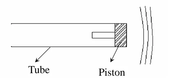
(28) more than one diameter apart and the radius a of the holes satisfies the inequality 0.01/. f < a < 10 / f , f is frequency in Hz, the acoustic impedance of. the sheet is given by 1 ( RA + jω M A ) N. ZA =. (39). where N is the number of holes, RA and M A are given by: RA =. ⎡t ⎛ π a 2 ⎞⎤ 2ωµ ⎢ + 2 ⎜1 − 2 ⎟ ⎥ b ⎠⎦ ⎝ ⎣a. ρ π a2. MA =. (40). ρ ⎡. ⎛ 2.5a ⎞ ⎤ t + 1.7a ⎜1 − 2 ⎟ ⎥ ⎢ b ⎠⎦ πa ⎣ ⎝. (41). 2. The parameter µ is the kinematic coefficient of viscosity. For air at 20o C and 0.76m Hg, µ ; 1.56 ×10−5 m 2 / s . A narrow slit is another acoustic element which can be modeled as an acoustic mass in series with the resistance. Fig. 9 is a simple diagram illustrates the geometry of such a slit. If the height inequality t < 0.003 / Z A = RA + jω M A =. t. of the slit in meters satisfies the. f , the acoustic impedance of the slit is given by. 12η l 6ρl + jω 3 5wt t w. (42). The parameter η is the viscosity coefficient. For air, η = 1.86 × 10−5 N gs / m 2 at. 20o C and 0.76m Hg.. Lumped Parameter Oscillator Model of a Duct When sound propagates inside of a rigid duct, a resonance phenomenon occurs. If the wavelength of the traveling wave is much larger than the diameter of the duct, the resonance properties will be governed by the pipe length and end conditions. When the wavelength becomes equal to, or smaller than the diameter of the pipe, two 15.

(29) and three-dimensional standing waves can occur. By matching the impedance of the loudspeaker and the duct at the end conditions, the resonant points can be calculated. First, consider a duct that is rigidly terminated at one end and is excited by a flat massless piston at the other. Fig. 10 shows a flat circular piston in one end of a circular tube of cross-section S , length l , and internal volume V = S l . Assuming that the piston is used to drive only low frequency content so that it produces a constant volume velocity, only plane waves will be produced. The pressure will take the form: p ( x) = Ae − jkx + Be + jkx. (43). The velocity has u ( x) =. 1 ⎡ Ae− jkx − Be + jkx ⎤⎦ ρc ⎣. (44). At the load, the ratio of the pressure p (l ) to the volume velocity U (l ) must be equal to the acoustical impedance Z A of the load. Thus we can write Z AL =. p (l ) p (l ) Ae − jk l + Be + jk l = = S U (l ) Su (l ) ⎡ Ae − jk l − Be + jk l ⎤⎦ ρc ⎣. (45). The acoustic impedance Z A seen by the ratio of the pressure p(0) at the source to the volume velocity U (0) emitted by the source. The equation can be wrote ZA =. p(0) p(0) = U (0) Su (0). (46). The impedance seen by the source is given by. ρc ρ c Z AL cos(k l ) + j ( S ) sin(k l ) ZA = × S ( ρ c ) cos(k l ) + jZ sin(k l ) S. (47). AL. If the terminating impedance at. Z = l. is omitted so that the duct radiates into. free air, it can be shown that approximation to the pressure at the end of the duct. 16.

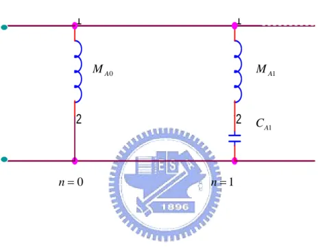
(30) is p ( l ). . The impedance Z AL =. ; 0. p (l ) = 0 . Thus the impedance seen by the source U (l ). is given by j ( ρ c ) sin(k l ) ρc S ZA = × = j tan(k l ) S ( ρ c ) cos(k l ) S S. ρc. (48). Resonance will occur as Im{Z A (0)} = 0. ⇒ kL = nπ , n=1,2,... ⇒ ωn = n. πc. (49). L. We seek an approximation of the form ZA (0) ≈ jω M A +. 1 1 ) at = j (ω M A − ωCA jω C A. the neighborhood of ω n . From Fig. 11, matching the resonance frequency and the slop of the two curves can do this. M AC A =. 1. ω n2. =. L2. (50). n 2π 2 c 2. d 1 [Im( Z A )] = M A + 2 = 2M A dω ωn CA ω =ω n. (51). From Eqs. (50) and (51). ρ0c S. sec 2 (kL). CA =. L ρ0 L 2 = sec (nπ ) = 2M A c S. (52). L2. 2S 2 SL = 2 2 n π c ρ0 L n π ρ0c 2 2. (53). 2 2. When n =1, the duct produces the first resonance MA =. ρ0 L 2S. =. 1 mass in the duct = 0.5 M A0 2. Thus the acoustic mass of the first resonant frequency can be lumped as 0.5 times acoustic mass of duct. CA =. 2 SL ≈ 0.2 compliance in the duct π 2 ρ0 c 2. The acoustic compliance of the first resonant frequency can be lumped as 0.2 times acoustic compliance of duct. 17.

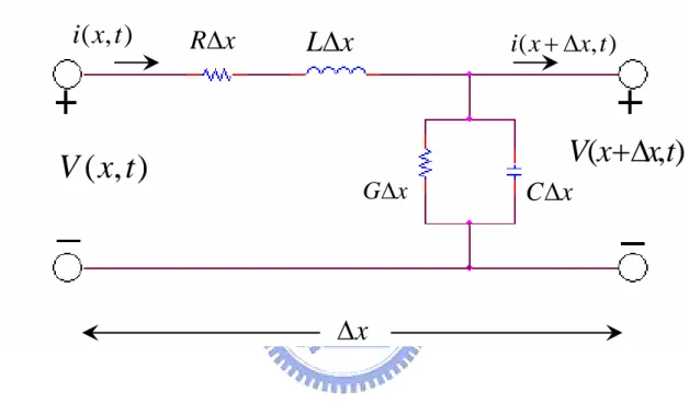
(31) The analogous circuit of the oscillator model of a duct is shown in Fig. 12.. Transmission Line Model of a Duct In this section, the theory of electromagnetic about transmission line is discussed. The transmission line can be represented by a simple equivalent circuit which is shown in Fig. 13. where R, resistance per unit length, in Ω / m ; L, inductance per unit length, in H / m ; G, conductance per unit length, in S / m ; C, capacitance per unit length, in F / m . For solving the circuit diagram, the following ordinary differential equations for phasors V ( x) and I ( x) : −. dV ( x) = ( R + jω L) I ( x) dx. (54). −. dI ( x) = (G + jωC )V ( x) dx. (55). These two equations are time-harmonic transmission-line equation. The two equation (54) and (55) above can be combined to solve for V ( x) and I ( x) . Two equations can be derived as: d 2V ( x) = γ 2V ( x) d 2x. (56). d 2 I ( x) = γ 2 I ( x) d 2x. (57). where γ = α + j β = ( R + jω L)(G + jωC ) is the propagation constant whose real and imaginary parts, α and β , are the attenuation constant and phase constant of the line. The solutions of Eqs. (56) and (57) are. V ( x) = V0+ e−γ x + V0− eγ x. (58). I ( x) = I 0+ e−γ x + I 0− eγ x. (59). 18.

(32) The ratio of the voltage and the current at any x-direction for an infinite line is independent of x and is called the characteristic impedance of the line. Z=. R + jω L. γ. =. γ G + jωC. =. R + jω L G + jωC. (60). For the case of the Lossless line (R=0, G=0), there are three special significance listed below: (a) Propagation constant:. γ = α + j β = jω LC α =0. (61). β = ω LC (b) Phase velocity: u=. ω 1 = β LC. (62). (c) Characteristic impedance: Z = R + jX = R=. L C. L C. (63). X =0. For acoustic system, phase velocity equals sound velocity. Therefore. β =k =. ω c. = ω LC. (64). γ = α + j β = jω LC = jk (α = 0). (65). Thus Eqs. (58) and (59) can be written as V ( x) = V0+ e− jkx + V0− e jkx. (66). I ( x) = I 0+ e− jkx + I 0− e jkx. (67). According to Eqs. (66) and (67), analysis is similar with Eqs. (43) and (44). 19.

(33) From the three special significance, L and C can be solved by the characteristic impedance of the duct is. ρc S. , and the phase velocity of the duct is c.. Thus, the two equations below can be combined to solve and the values of L and C can be got.. ρc S. c=. =. L C. (68). 1 LC. (69). where c is sound velocity; l is the length of the duct; S is the cross-section area. The detail of the transmission line can be found [8].. Two-Port Model of a Duct Two port networks are another type of model which is widely used in analysis of the circuit diagram. They are used to model transistors, transformers, and other circuit blocks. In this section, the duct is modeled by a two-port network in which voltage is analogous to pressure and current is analogous to volume velocity. The geometry of the duct is shown in Fig. 10. Two equations can be formulated as p ( x) = Ae − jkx + Be+ jkx U ( x) = Su ( x) =. S ⎡ Ae − jkx − Be + jkx ⎤⎦ ρc ⎣. From the above two equations, Eqs.46 and Eqs.47, the transmission matrix can be formulated as ⎡ cos(k l ) ⎡ p1 ⎤ ⎢ ⎢U ⎥ = ⎢ S ⎣ 1⎦ ⎢ j sin(k l ) ⎢⎣ ρ c. j. ρc. ⎤ sin(k l ) ⎥ ⎡p ⎤ S ⎥⎢ 2⎥ U cos(k l ) ⎥ ⎣ 2 ⎦ ⎥⎦. (70). where k is wave number, k = 2π / c ; l is the length of the duct; S is the cross-section area. 20.

(34) For the convenience of the analysis of the circuit diagram, the impedance matrix is adopted. And the two equations can be defined as p1 = z11U1 + z12U 2 p2 = z21U1 + z22U 2 Rewriting the two equations above in matrix form, we obtain P = ΖU. where the matrix ⎡z Ζ = ⎢ 11 ⎣ z21. z12 ⎤ is called the impedance matrix. z22 ⎥⎦. From [9], the conversion between the transmission and the impedance matrix can be easily solved. After the transformation, the impedance matrix can be formulated as: ⎡ ρc −j cot(k l ) ⎡ p1 ⎤ ⎢ S ⎢ p ⎥ = ⎢ ρc ⎣ 2 ⎦ ⎢− j csc(k l ) ⎢⎣ S. ρc. ⎤ csc(k l ) ⎥ ⎡U 1 ⎤ S ⎥⎢ ⎥ U ρc cot(k l ) ⎥ ⎣ 2 ⎦ j ⎥ S ⎦. j. An equivalent circuit of a two-port model is shown in Fig. 14.. 21. (71).

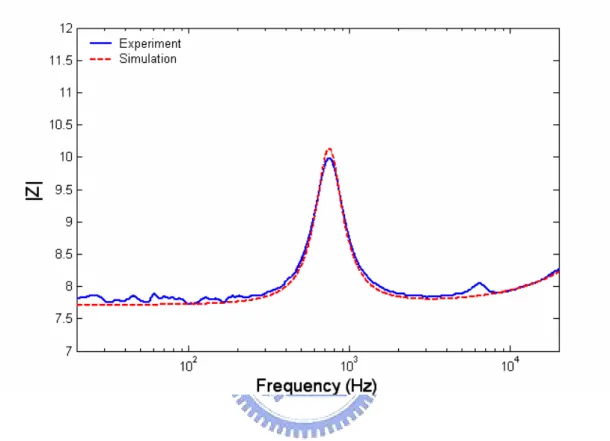
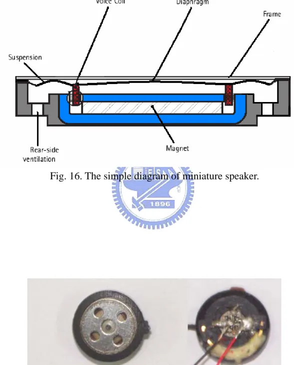
(35) 2. Simulation and experiment of results In this section, the experiment results will be used to analyze miniature speaker and compared with the simulation results. Something that affects the performance of miniature speaker can be clearly realized by experiment results. A real example of mobile phone is presented and the structure of the mobile phone that causes some effects on the miniature speaker will be discussed. The theory of electroacoustics is used to simulate the conditions that the miniature speaker placed in mobile phone.. 2.1 Parameter identification of miniature speakers From the last section, Thiele and Small parameters of the loudspeaker can be got by the procedures of measurement. In order to check these values are correct or not. These values must be taken into electro-mechano-acoustical analogous circuit and the simulation results will be compared with the experiment results. The comparison results are shown in Fig. 15. The testing speaker is the products of Merry Company. Its data number is DSH456.. The type of loudspeaker is the miniature speaker.. From the Fig. 15., the simulation results can approximately fit the experiment results. Thus Thiele and Small parameters of the miniature speaker can be used to model its dynamic response. The simple diagram of miniature speaker is shown in Fig. 16. and the real object of miniature speaker is shown in Fig. 17. The basic features can be observed from the Fig. 18. and Fig.19. The voice coil is attached to the diaphragm. A frame is fixed above the diaphragm.. Ports in the rear side of the speaker provide ventilation to the. rear enclosure. Some damping materials are located on the ports. These features are different from the conventional loudspeaker. What do they cause some effects on the speaker?. According to the experiment results, the obvious effects can be. 22.

(36) observed from the impedance and pressure frequency response. In order to analysis these effects, three cases are split and the experiments will be done individually. The three cases are listed below: Case 1: the original speaker Case 2: the speaker without the damping material Case 3: the speaker without the damping material and the frame Fig. 18. is the back of the miniature speaker and the view of case 1 and case 2. Fig. 19. is the front of the miniature speaker and the view of case 2 and case 3. The impedance and sound pressure frequency response of the three cases are shown in Fig. 20. and Fig. 21.. From the impedance response comparison, the. amplitude of the first resonant frequency of the three cases is different with each other. This phenomenon indicates that the damping material and the frame affect the amplitude of the first resonant frequency. And the damping material causes more effects than the frame.. Why does the frame affect the amplitude of the first resonant. frequency? There is the mesh material that is located above the frame in the Fig. 19. It is also the damping material. Frame attached to the diaphragm are important factors that influence the radiated sound field. [5] presents numerical models of miniature loudspeakers in various conditions of frame and presents an analysis of the structure vibration of the diaphragm coupled with the radiated sound field. This paper pointed out that if there are more holes in the frame, the frame will not cause more effects on the sound pressure frequency response. From the sound pressure frequency response in the Fig. 21., the amplitude of the first resonant frequency of three cases is different. This can illustrates the damping material could decrease the dB of the sound pressure level in the first resonant frequency. In 13k Hz, the sound pressure level of the case 3 is lower than the other two cases, because the mesh material in the frame affects the value of dB. 23.

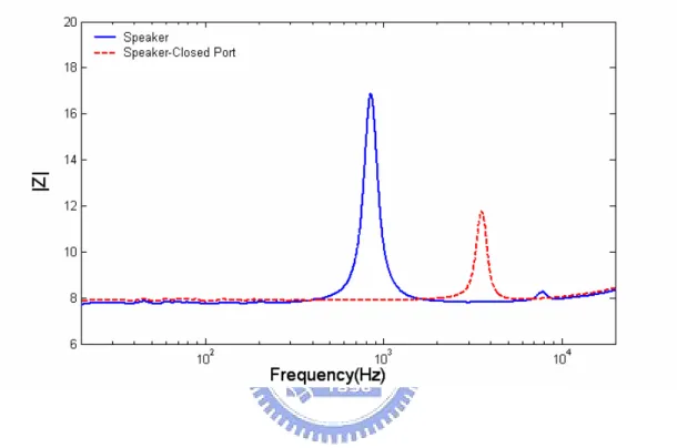
(37) A resonant peak is found in the about 6~7k Hz from Fig. 20. The resonance happened in the 6~7 kHz is caused by the port embedded in the rear side of the speaker and the small space of the cavity in the back of the diaphragm. Fig. 22. is the experiment results that can prove the resonance caused by the port embedded in the rear side of the speaker and the small space of the cavity in the rear of the diaphragm.. When the port embedded in the rear side of the speaker is closed, the. peak in 6~7k Hz disappeared. And the first resonance frequency is shifted to the high frequency. The speaker is like to be mounted in the closed-box. Thus the stiffness of the speaker is raised, the first resonance frequency rose. From the concept of electroacoustics, the effects can be explained by this: the port that can be modeled as the acoustic mass and the resistance and the small space of the cavity can be modeled as the acoustic compliance, so the acoustic mass and the acoustic compliance cause the resonance when the imaginary impedance is zero. The resonant frequency is also called the Helmholtz resonance frequency at which the acoustic impedance is zero. In order to prevent this effect, the dimension of the port can be change large. Then the peak of the resonance will be shifted to more high frequency. From the discussions above, the damping material plays an important role in the performance of miniature speakers. For the demand of application, the damping material can be selected to change the dynamic response of the speakers that you need. Figure 23. (a), (b), (c), (d), (e), (f), (g), (h) are the directivity plot of the miniature speaker. Its measuring range of frequency is from 500 Hz to 11k Hz. The speaker is not mounted in the infinite baffle.. From the polar plot of the directivity in Fig. 23.,. the directivity of the miniature is omnidirectiona.. 24.

(38) Using Thiele and Small parameters can roughly calculate sensitivity and efficiency for miniature speakers. The pressure sensitivity of loudspeakers is calculated by Eqs. 72. V p1sens =. ρ0 Bl 2π S D RE M AS. (72). The SPL sensitivity of SPL1Vsens and SPL1W sens is calculated by Eqs. 73 and Eqs. 74. ⎡ p1V ⎤ V = 20 log ⎢ sens ⎥ dB . SPL1sens ⎢⎣ Pref ⎥⎦ 1W sens. SPL. (73). V ⎡ p1sens RE ⎤ = 20 log ⎢ ⎥ dB ⎥⎦ ⎣⎢ Pref. (74). where SPL1Vsens is SPL sensitivity of 1V rms. input voltage; SPL1W is SPL sens RE V rms. input voltage; pref = 2 ×10−5 Pa.. sensitivity of. The efficiency of loudspeakers is calculated by Eqs. 75 and 76. η=. PAR PE. (75). where PAR is the acoustic power; PE is the electrical power.. η=. ρ0 B 2 l 2 S D2 2 2π c RE M MS. (76). For a example of merry speaker, its Thiele and Small parameters are listed below Bl = 0.3254. S D = 0.0000785m 2. RE = 7.81Ω. η=. M MS = 0.021263g. ρ0 B l S = 0.0104% 2 2π c RE M MS 2 2. 2 D. ⎡ p1V ⎤ V SPL1sens = 20 log ⎢ sens ⎥ dB = 63dB ⎢⎣ Pref ⎥⎦ ⎡ p1V R W = 20 log ⎢ sens E SPL1sens ⎢⎣ Pref. ⎤ ⎥ dB = 72dB ⎥⎦. 25.

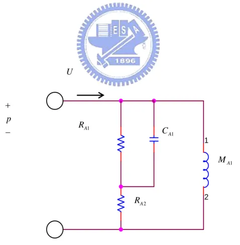
(39) From above calculation of sensitivity and efficiency, miniature speaker has smaller sensitivity and efficiency than conventional loudspeakers.. The efficiency and. sensitivity can be increased by increasing the Bl , by increasing the diaphragm area, by decreasing the voice-coil resistance, and by decreasing the total moving mass.. 2.2 Modeling of the miniature speaker in mobile phones In the preview section, the electro-mechano-acoustical analogous circuit and the concept of electroacoustics are discussed.. In acoustical system for loudspeaker,. something must be cared is Z AB and Z AF . The Z AB and Z AF model the acoustical impedance on the front and rear of the diaphragm. The example of the mobile phone is shown in Fig 24. The Z AB and Z AF are the complex-loading conditions. From the Fig 24, the structure of the mobile phone can clearly been realized. The structure in the rear and front of the speaker that causes some effects on the sound field. These structures of acoustical properties will be lumped to the analogous circuit in the acoustic system. These analogy circuits are composed of the acoustic components like duct, slit, port or cavity, etc. The front of the diaphragm is covered by a method perforated cover. The acoustic impedance of the mesh screen can be modeled by a series of acoustic mass and resistance. The value of the acoustic mass and resistance can be calculated by the Eqs. 39, 40 and 41.. We can image that the volume velocity emitted by the. diaphragm flows through the mesh screen. When the speaker is placed in mobile phone, there is a small space in the front of speaker. The acoustic impedance of the small space can be model an acoustical compliance and it can be calculated by Eqs. 27. So the volume velocity will compress the air in the small space, then flow through the port that is placed on the side of small space. The port exhibits an acoustic resistance and mass. The acoustic impedance of the port can be calculated by Eq 42. 26.

(40) The volume velocity flows through the port and flows into the duct. In order to model the duct, lumped parameter oscillator model and the transmission line model can be used to model the dynamic response of the duct. But lumped parameter oscillator model is used here to simulate. The analogous circuit of lumped parameter oscillator model is shown in Fig. 13. In the export of the duct, something can be found that the area of the export of the duct is less than the cross-sectional area of the duct. When the volume velocity flows out the export of the duct, the air will be compressed in the export of the duct. Thus the dynamic behavior is like an acoustic compliance. After the volume velocity flows out the export of the duct, it will flow through the port and radiates the sound. The port exhibits an acoustic resistance and mass. The acoustic impedance of the port can be calculated by Eqs. 42. Final, there is the radiation impedance between the export of the port and the medium.. The analogous circuit of the radiation. impedance is shown in Fig 6. The radiation impedance is the radiation impedance of the piston in a tube. Its analogous parameters can be calculated by Eqs. 35, 36, 37 and 38. The rear of the diaphragm is like a closed box and there are two ports embedded in the rear of speaker. The closed box can be modeled by an acoustic compliance. The parameters of the acoustic compliance can be calculated by Eqs. 27. The port can be modeled by a series of acoustic mass and resistance. The back volume velocity emitted by the diaphragm compresses the air in the box and flows through the port. The rear of the speaker is like a box that the acoustic impedance is modeled by an acoustical compliance and its analogous parameters can be calculated by Eqs. 27. The analogous circuit of the electro-mechano-acoustical analogous circuit of miniature speaker placed in mobile phone is shown in Fig. 25. The structure of the front of the speaker is shown in Fig. 26. (a). The analogous circuit of Z AF is shown 27.

(41) in Fig. 26. (b). The structure of the rear of the speaker is shown in Fig. 27 (a). The analogous circuit of Z AB is shown in Fig. 27 (b).. And the circuit elements are. defined below:. RAF and MAF. : the acoustic impedance of the frame. We can approximately compute the values by the Eqs. (39), (40) and (41).. CAF. : the acoustic compliance between the frame and the diaphragm. We can compute the value by the Eqs. (27). CFB1. : the acoustic compliance in the front of the speaker. It is like a box. We can compute the value by the Eqs. (27). RAP1 and MAP1. : the acoustic impedance of the port around CFB1. We can approximately compute the value by the Eqs. (42). MAL1. : the acoustic mass of the duct. We can compute the value by the Eqs. (29).. MAL2 and CAL2. : Because of the natural resonance of the duct, we can model that by Oscillator Model of a Duct, and compute the values by Eqs. (52) and (53).. RAP2 and MAP2. : the acoustic impedance of the port in the exportation of the duct. We can approximately compute the value by the Eqs. (42).. CAL. : the acoustic compliance in the exportation of the duct. We can approximately compute the values by Eqs. (29). M1, R1, R2 and C1: the element of the radiation impedance. We can approximately compute the values by Eqs. (35), (36), (37) and (38). RBP1 and MBP1. : the acoustic impedance of the port embedded in the rear of the 28.

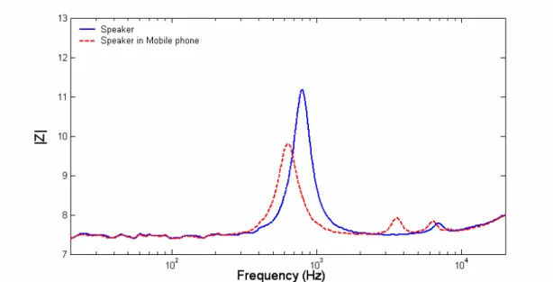
(42) speaker. We can approximately compute the value by the Eqs. (42) CBB1. : the acoustic compliance of the cavity in the rear of the diaphragm. We can approximately compute the values by Eqs. (27). CBB2. : the acoustic compliance of the cavity in the rear of the speaker. We can approximately compute the values by Eqs. (27). RBP2 and MBP2: the acoustic impedance of the port embedded in the cavity. We can approximately compute the value by the Eqs. (42).. Fig. 28. is the impedance response comparison of speaker and speaker placed in mobile phone and the impedance response is the experiment results.. The first. resonant frequency of the speaker placed in mobile phone is lower than speaker that is not placed in mobile phone. This is because the acoustic mass of Z AF and Z AB reflected to the electrical system cause the total mass increasingly. Thus the first resonance frequency is shifted to low frequency. This effect can be realize from the below equation.. ω0 = if. 1 MC M or C ↑ , ω0 ↓. From the Fig 28, there is a resonance at about 3.5k Hz. The resonance is caused by the compliance of the small space in the front of the speaker and the mass of the duct and the port.. The resonance at about 6.5 kHz is caused by the. compliance of box in the rear of the diaphragm and the mass of the port. Figure 29 is the frequency response comparison of speaker and speaker placed in mobile phone. The resonance at about 17k Hz is caused by the natural resonance of the duct. 29.

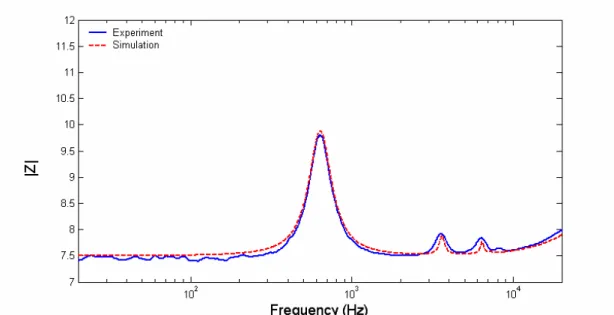
(43) The Pspice is used to construct the electro-mechano-acoustical analogous circuit according to the analysis of the Z AB and Z AF by using the theory of the electroacoustics and do the simulation of impedance and frequency response. Figure 30 and 31 are the simulation results of the impedance and sound pressure frequency response. The simulation results can approximately fit the experiment results.. Ear-coupling Simulation In this section, the B&K products of Wideband Ear Simulator for Telephonometry Type 4195 is taken to analyze realistic telephone receive response measurements. The two grades of well-defined leakage make it possible to simulate late the average real loss for telephone handsets which are held either comfortably tight (low-leak pinna) or lossely (high leak pinna) against the human ear. This product provides the equivalent circuit to model low-leak and high-leak conditions. The equivalent circuit can be used in the frequency range 100 Hz to 8k Hz. The equivalent circuit diagram is shown in Fig. 32.. The acoustic impedance. simulation results are shown in Fig. 33.. The mobile phone coupled with low-leak and high-leak Pinna simulation results are shown in Fig. 34... 30.

(44) 3. Bass-enhanced design for the miniature speakers In this section, the theories of vented-box and passive-radiator design method are reviewed. Using the concept of the theory, the enclosure of the speaker can be designed to enhance the bass response of the speaker.. 3.1 The vented-box design Figure 35 is a simple diagram of vented-box design. There is a tube with a circular cross section installed in the front of the enclosure. The air in the vent is modeled as an acoustic mass. The acoustic mass and the acoustic compliance of the air in the enclosure form a Helmholtz resonator which can improve the bass response of the system. The EMA analogous circuit of the vented-box in low-frequency is shown in Fig. 36. In the acoustic circuit, the resistance RAL models air-leak losses in the enclosure. The mass M AP models the air in the port which is a tube with a cross-section area S P and a length l . The tube is flanged at one end and unflanged at the other. The acoustic mass of the air in the port is modeled by M AP =. ρ ⎛. SP ⎞ ⎜⎜ l + 1.462 ⎟ SP ⎝ π ⎟⎠. (77). The Helmholtz frequency is given by. ωP = 2π f =. 1. (78). M AP C AB. where C AB is the compliance of the air in the enclosure modeled by C AB =. VAB ρc2. (79). where VAB is the effective acoustic compliance of the air in the enclosure For the convenience of getting the volume velocity, the EMA analogous circuit is. 31.

(45) transformed to acoustical analogous circuit.. The acoustical analogous circuit is. shown in Fig. 37. (where M AC is the sum of M AD and M A1 ; M AD is the acoustical equivalent of M MD ).. From the acoustical analogous circuit, the volume velocity. transfer function can be derived as s 3 ω04 Bl e U= S D RE M AS ( s ω0 ) 4 + a3 ( s ω0 )3 + a2 ( s ω0 ) 2 + a1 ( s ω0 ) + 1 a1 =. where. α=. 1. QL h. +. h QTS. C AS VAS = C AB VAB. QL =. a2 = h=. α +1 h. +h+. ωB f B = ωs fs. 1 QTS QL. (80). a3 =. 1. QTS h. +. h QL. ω0 = 2π f 0 = ωsωB. RAL C AB = ω B RALC AB = RAL M AP ωB M AP. The on-axis pressure can be calculated by the equation p =. ρ sU . After some 2π r. simplification, the expression for the on-axis pressure can be formulated as. p=. ρ Bl e G ( s) 2π r S D RE M AS. (81). where G ( s ) is the vented-box on-axis pressure transfer function that can be formulated as. G ( s) =. s 3 ω04 ( s ω0 ) 4 + a3 ( s ω0 )3 + a2 ( s ω0 ) 2 + a1 ( s ω0 ) + 1. The pressure transfer function is a fourth-order, high-pass filter function.. At low. frequency, the bode magnitude plot exhibits an asymptotic slope of +80 dB per decade. The coefficients of a1 , a2 and a3 can be decided to design the shape of the Bode plot.. The numerical value of these coefficients defines the vented-box system. alignment. In this paper, these alignments will not be discussed. And the detail of the vented-box system alignment is clearly discussed by Small [10]. .. 32.

(46) 3.2 The passive-radiator design A passive radiator design of the loudspeaker which is the concept of the vented-box design extends.. The method is to replace the vent in the vented-box with. a passive driver that is no voice coil. The simple diagram is shown in Fig. 38. The low frequency Norton form of the acoustical analogous circuit is shown in Fig. 39. The acoustical analogous circuit is the simplification of the EMA analogous circuit. For the convenience of the analysis, the acoustical system is adopted. There is some difference between the analogous circuit of vented-box and passive radiator. In the acoustical analogous circuit of the vented-box, the port mass is replaced by a series mass M AP , resistance RAP , compliance C AP representing the acoustical analogous circuit of the passive radiator. From the acoustical analogous circuit of the passive radiator, the output volume velocity can be derived as:. U=. SDe RAE C s S e RAE C AB s × AB = D Bl Z A1 + 1/ Z A 2 Z A 2 Bl 1 + Z A1Z A 2. where. Z A1 = M AS s + RAE + RAS + Z A 2 = C AB s +. (82). 1. (83). C AS s. 1 1 + RAL M AP s + RAP + 1. (84) C AP s. The impedance Z A1 can be formulated as Z A1 =. where. ωs =. 1. M AS C AS. ( s ωs ) 2 + ( 1. QTS C AS s. QTS =. )( s ωs ) + 1. 1. ωs RAT C AS. RAT = RAE + RAS. And the Z A 2 can be written. Z A2. (1 + 1 ) ⎡ ( s ωB ) 2 + ( 1 )( s ωB ) ⎤ δ ⎢⎣ QL ⎥⎦ ( s ωP )2 = + M AP s M AP s ⎡( s ωP ) 2 + ( 1 )( s ωP ) + 1⎤ QP ⎣⎢ ⎦⎥ 33.

(47) where. ωP = δ=. 1. QP =. M AP C AP. C AP C AB. 1. QL = ωB RALC AB. ωP RAP C AP. ωB = ωP 1 + δ. For the simplification of the transfer function of the volume velocity, the box losses are neglected. So RAL → ∞ and QL → ∞ are defined. The transfer function of the on-axis pressure can be calculated.. p=. ρ ρ Bl e sU = G ( s) 2π r 2π S D RE M AS. (85). ( s ω0 ) ⎡⎣( s ω0 ). + (ωP ω0 ) 2 ⎤ ⎦ G ( s) = 4 3 2 ( s ω0 ) + a3 ( s ω0 ) + a2 ( s ω0 ) + a1 ( s ω0 ) + 1 2. 2. where. ( s ω0 ) ⎡⎢( s ω0 ). +β. ⎤ 1 + α + δ ⎥⎦ ⎣ = ( s ω0 ) 4 + a3 ( s ω0 )3 + a2 ( s ω0 ) 2 + a1 ( s ω0 ) + 1 2. ω0 = ω s. 1/ 4. β (1 + α + δ ). a1 =. (1 + δ ) β (1 + α + δ )3 4 QTS. a3 =. 1 (1 + α + δ )1 4 β QTS. 2. β = ωP ωs a2 =. α = C AS C AB. ⎡ 1+ α ⎤ ⎢ (1 + δ ) β + β ⎥ (1 + α + δ ) ⎣ ⎦ 1. As δ → ∞ , the transfer function of on-axis pressure of the passive radiator approaches that of the vented-box. The major difference between the vented-box and passive radiator is that two of these zeros of the numerator of the passive radiator. If RAP = 0 and ω = ω p , the transfer function is zero. response exhibits a notch at ω = ω p .. And the system. For design the passive radiator, the notch. frequency should be well below the system cutoff frequency. The effect of the notch generally is to sharpen the corner of the frequency response characteristic and to give 34.

(48) a steeper initial cutoff slope compared to the equivalent vented-box system. The alignment of the passive radiator will not be discussed in this paper. And the detail of the passive radiator system alignment is clearly discussed by Small [11].. 3.3 Simulation results When the loudspeaker is placed in the closed box, the stiffness of the closed-box system will increase. And the first resonance frequency of the closed-box system will rise to the high frequency. Fig. 40. is the frequency response comparison of the infinite baffle and closed-box. From the Fig. 40., the performance of the closed-box system in low frequency is bad than the infinite baffle for a small volume of box. Figure 41 is a simple simulation of the impedance response of the vented-box system.. The null in the impedance plot is at the Helmholtz resonance frequency that. is caused by the acoustic compliance of the volume of air and the acoustic mass of the vent.. Fig 42 is the simulation of the frequency response of the vented-box. The. volume velocity emitted by the diaphragm exhibits a null at the Helmholtz frequency and the volume velocity emitted by port is maximum. The total volume velocity is the sum of the volume velocity emitted by the diaphragm and the port. Figure 43 is the frequency response comparison of infinite baffle and the vented-box system.. The bass response of the vented-box is great than that of infinite. baffle. Figure 44 is the simulation frequency response of the passive radiator system. The notch at the total frequency response is the resonant frequency of the passive diaphragm. The notch frequency should be below the cut-off frequency for the passive radiator design. From Fig 44, the notch frequency is below the cut-off frequency, so it is a well design. Figure 45 is the frequency response comparison of infinite baffle and 35.

(49) passive-radiator system.. The bass response of the passive radiator is great than that. of infinite baffle. The alignments are not adopted to design the passive radiator and the vented-box system.. Because the miniature speaker has higher QTS than the. conventional loudspeaker, the miniature speaker is not suitable to design according to the alignments of the vented-box and the passive-radiator. From the discussion above, the simple models of the vented-box and the passive radiator have been constructed. Next, the miniature speaker will be taken to design the sample of the vented-box and the passive radiator, and the design of the sample can be used to realize in mobile phone. Figure 46 is the 3-D diagram of the vented-box design. The parameters of the vented-box design are limited to realization in mobile phone. The dimension of the vented-box is the main reason. The simulation results of frequency response for infinite baffle and vented-box design are shown in Fig. 47. From the Fig. 47., the bass response of the vented-box design is great than the infinite baffle.. Fig. 48. is. the frequency response comparison of vented box for vent open and vent close. The vent close is like the closed-box system. The bass response of the vented-box design is great than the closed-box system. Figure 49 is the 3-D diagram of the passive radiator design. The parameters of the passive radiator design are limited to realization in mobile phone. compliance of the passive diaphragm is not easily determined. compliance just can be determined by measurement.. But the. The value of the. Fig. 50. is the frequency. response comparison for infinite baffle and passive radiator design. The frequency response of the passive radiator performs well as the infinite baffle. Fig. 51. is the frequency response comparison of passive radiator design and the passive radiator without passive diaphragm. The passive radiator design without passive diaphragm 36.

(50) is like the closed-box system.. The bass response of the passive radiator design is. great than the closed-box system. For the simulation of vented-box and passive radiator design, there is big peak in 15 kHz. That is caused by the acoustic compliance of the small space in the front of the speaker and the acoustic mass of the port around the small space.. By placing. the damping material in the export of the port, the amplitude of the peak will decrease.. 37.

(51) 4. Conclusions There are many different features between miniature speakers and convention loudspeakers. The analysis of miniature speakers is discussed in this paper. These features that cause effects on the performance of miniature speaker are proven from the experiment results.. In connection with different applications, these features can. dominate the performance of miniature speakers to arrive the demands of user. Thiele and Small parameters are important indexes. These parameters can make us to realize the difference between miniature speakers and convention loudspeakers. The inductance of voice-coil is an example. For convention loudspeakers, the high frequency inductance effect is very great. This phenomenon can not be represented by a linear inductance. However, the inductance of voice-coil for miniature speaker is very small.. Thus the high frequency inductance effect can be approximately. modeled by a linear inductance.. The sensitivity and efficiency for miniature. speakers are very smaller than convention loudspeakers.. The efficiency and. sensitivity can be increased by increasing the Bl , by increasing the diaphragm area, by decreasing the voice-coil resistance, and by decreasing the total moving mass. However, increasing Bl is the best method for miniature speaker. The EMA analogous circuit is established to analyze the dynamic response of the loudspeaker.. When the loudspeaker is placed in the complex enclosure, we can. focus on the acoustical system and use lumped parameter method to model the acoustical impedance of the structure of the enclosure. The acoustical impedance is lumped to the electrical element. The overall dynamic response of the loudspeaker can be easily solved by the circuit analysis. For mobile phone, ear-coupling condition is an important index. The low-leak and high-leak conditions are simulated to analyze the dynamic response of mobile. 38.

(52) phone in different ear-coupled conditions. For enhancing the bass response of miniature speakers placed in mobile phone, the concept of the vented-box and passive radiator methods is reviewed in this paper. From the theory analysis and simulation results, the vented-box and passive radiator methods can efficiently improve the bass response of the loudspeaker. However, the dimension of the mobile phone is limited.. Thus the best performance of the bass. response for the vented-box and passive radiator design can not be developed well. However, the bass response is still enhanced. For the passive radiator design, one thing must be noticed is that the passive diaphragm can be choosing to reach the best performance of the bass response The vented-box and passive radiator design for the mobile phone conferred above is just in the process of simulation. In the future, we will realize this concept to develop a real enclosure and prove that the vented-box and passive radiator design can really enhance the bass response of the loudspeaker from the experiment results.. 39.