大型時空資料庫中拓樸樣式探勘之漸進式維護

國

立

交

通

大

學

多媒體工程研究所

碩

士

論

文

大型時空資料庫中拓撲樣式探勘之漸進式維護

Incremental Maintenance of Topological Patterns in Large

Spatial-Temporal Database

研 究 生：吳昭瑩

指導教授：李素瑛 教授

大型時空資料庫中拓撲樣式探勘之漸進式維護

Incremental Maintenance of Topological Patterns in Large

Spatial-Temporal Database

研 究 生：吳昭瑩 Student：Chao-Ying Wu

指導教授：李素瑛 Advisor：Suh-Yin Lee

國 立 交 通 大 學

多 媒 體 工 程 研 究 所

碩 士 論 文

A Thesis

Submitted to Institute of MultimediaEngineering College of Computer Science

National Chiao Tung University in partial Fulfillment of the Requirements

for the Degree of Master

in

Computer Science August 2011

Hsinchu, Taiwan, Republic of China

i

大型時空資料庫中拓撲樣式探勘之漸進式維護

研究生：吳昭瑩

指導老師：李素瑛 教授

國立交通大學多媒體工程研究所

摘要

在許多空間時間資料庫的生活應用，例如環境生態分析、氣象分析、位置基 礎分析，大都隨著時間變化做增量的更新。當資料庫增量更新後，有些已發現的 拓撲樣式會無效，而有些新的拓撲樣式會出現。 當新的事件加入資料庫，假如每一次的更新都必須重新探勘拓撲樣式，將是 一件既沒效率且不切實際的工作。儘管最近有學者提出維護拓撲樣式的方法，而 且我們也可以應用既有探勘靜態資料庫的演算法重新探勘更新後的資料庫。然而， 既存的演算法並不是非常有效率。 在大型時空資料庫中拓撲樣式探勘之漸進式維護是一件艱鉅的工作，因為拓 撲樣式探勘相較一般項目集樣式是比較複雜的。在這篇論文，我們提出一個演算 法，Inc_TMiner，主要是設計在增量的時空資料庫中維護拓撲樣式。在合成資料 的實驗結果顯示 Inc_TMiner 在執行時間優於之前的漸進式演算法，也優於利用 現有探勘靜態資料庫的演算法重新探勘更新後的資料庫。 關鍵字：資料探勘, 增量式探勘, 拓撲樣式, 時間樣式, 時空資料庫.

ii

Incremental Maintenance of Topological Patterns in Large

Spatial-Temporal Database

Student: Chao-Ying Wu

Advisor: Prof. Suh-Yin Lee

Institute of Multimedia Engineering National Chiao Tung University

ABSTRACT

Spatial temporal data mining is an important research area with many interesting topics, such as ecology analysis, meteorology analysis, location-based analysis and so forth. Most spatial temporal databases are updating incrementally with time. Some discovered topological patterns may be invalidated and some new topological patterns may be introduced by the evolution of databases. When new instances are inserted into the database, we can re-mine topological patterns from scratch each time using the existing static algorithms. Some researches on the maintenance of topological patterns in an incremental manner are proposed. However, all static algorithms and incremental algorithms are incompetent and not scalable.

In this thesis, an efficient algorithm, Inc_TMiner (Incremental Topology Miner) is developed to incrementally maintain topological patterns from spatial-temporal databases. The experimental results on synthetic datasets indicate that Inc_TMiner significantly outperforms the static algorithms and the existing incremental algorithm in execution time and possesses graceful scalability.

Keyword: data mining, incremental mining, topological pattern, collocation pattern, spatial-temporal database.

iii

Acknowledgement

I greatly appreciate the kind guidance of my advisor, Prof. Suh-Yin Lee. She not only helps with my research but also inspires and takes care of me. Without her graceful suggestion and encouragement, I cannot complete the thesis. Besides I want to give my thanks to all members in the Information System Laboratory for their suggestion and instruction, especially Mr. Yi-Cheng Chen, Miss Yu-Jiun Liu, Mr. Ji-Chiang Jiang, Mr. Cheng-Yi Peng, Mr. Yee-Choy Chean, and Mr Li-Wu Tsai.

Finally I would like to express my deepest appreciation to my parents, Mr. Ming-Fang Wu and Mrs. Tu-Xiang Huang and my brother Chung-Ying Wu. This thesis is dedicated to them.

iv

Table of Contents

ABSTRACT(Chinese) ... i ABSTRACT(English) ... ii Acknowledgement ... iii Chapter 1. Introduction ... 1

1.1 Introduction and Motivation ... 1

1.2 Outline of the Thesis ... 3

Chapter 2. Related Works ... 4

Chapter 3. Problem Definitions ... 6

Chapter 4. Basic Concepts of the Static Algorithms ... 9

4.1 Topology Miner... 9

4.1.1 Summary Structure ... 10

4.1.2 Concept of Projected Database ... 12

4.1.3 Construction of Projected Database ... 13

4.1.4 Mining Topological Patterns ... 14

4.2 Join-less Collocation Miner ... 18

4.2.1 Neighborhood Materialization ... 19

4.2.2 Join-less Collocation Mining Algorithm ... 20

Chapter 5. Proposed Algorithm: Inc_TMiner ... 24

5.1 Basic Definitions of Updated Database ... 24

5.2 The Basic Concept of Inc_TMiner... 27

5.3 The Updating Process of Inc_TMiner ... 29

5.3.1 Cases of Updating Process ... 29

5.3.2 Inc_TMiner Algorithm ... 30

Chapter 6. Experimental results and performance study ... 41

6.1 Data Generator ... 42

6.2 Performance ... 44

6.2.1 Effect of Cross Ratio ... 44

6.2.2 Effect of Incre Ratio ... 45

6.2.3 Effect of Data Size ... 46

6.2.4 Effect of Prevalence Threshold ... 48

Chapter 7. Conclusion ... 50

v

List of Figures

Figure 3-1: Examples of topological patterns ... 7

Figure 4-1: An example of the spatial temporal database ... 10

Figure 4-2: The summary structure with the two indices CFI and FCI. ... 12

Figure 4-3: The projected database of <𝑓1> ... 13

Figure 4-4: The projected database of < 𝑓1, 𝑓2 > ... 14

Figure 4-5: An example of mining star-like patterns ... 15

Figure 4-6: An example of mining clique-like patterns . ... 16

Figure 4-7: The framework of Topology Miner . ... 17

Figure 4-8: The concept of candidate-maintenance-test with Apriori Property pruning. ... 18

Figure 4-9: An example to materialize star neighbor relationships ... 19

Figure 4-10: The pseudo code of Join-less Collocation Miner ... 21

Figure 4-11: The process of mining topological patterns. ... 22

Figure 5-1: The classification of the databases. ... 24

Figure 5-2: The concepts of Non_Cross database and Cross database ... 25

Figure 5-3: An example of the extended database EDB ... 25

Figure 5-4: An example of count information CI ... 26

Figure 5-5: An example of (a) the original database (b) star neighborhood. ... 28

Figure 5-6: The framework of Inc_TMiner. ... 31

Figure 5-7: The pseudo code of Inc_TMiner. ... 32

Figure 5-8: An example of the updated database DB’ and the extend database EDB 33 Figure 5-9: The star neighborhood of the extended database. ... 34

Figure 5-10: The count information after database updated ... 35

Figure 5-11: An example of count information after the Star Mining Phase. ... 36

Figure 5-12: The process of determining the frequency of pattern <𝑓1,𝑓2,𝑓3> ... 37

Figure 5-13: The process of determining the frequency of pattern <𝑓1,𝑓3,𝑓4> ... 38

Figure 5-14: The process of determining the frequency of pattern <𝑓2,𝑓3,𝑓4> ... 39

Figure 5-15: The flowchart of Inc_TMiner... 40

Figure 6-1: Parameters of synthetic data generator ... 42

Figure 6-2: The effect of Cross Ratio ... 45

Figure 6-3: The effect of Incre Ratio ... 46

Figure 6-4: The effect of Data Size v.s. Runtime ... 47

Figure 6-5: The effect of Data Size between the incremental algorithms v.s. Runtime ... 47

vi

Figure 6-7: The effect of min_prevalence V.S. Runtime ... 49 Figure 6-8: The effect of min_prevalence V.S. Memory Usage ... 49

1

Chapter 1. Introduction

1.1 Introduction and Motivation

In recent years, spatial-temporal data mining has received considerable attentions. One important research topic in spatial-temporal data mining is mining topological patterns, also called colocation patterns. Mining topological patterns is an interesting and essential data mining technique with broad applications, such as ecology analysis, location-based analysis and meteorology analysis, to name a few. Many efficient algorithms [2, 3, 4, 5, 6, 7] proposed so far have good performances of discovering topological patterns from static databases.

However, the assumption of having a static database may not be considered in some applications, since most databases usually grow incrementally over time in our daily life. Take meteorology analysis as an example, weather usually changes every day, such as “in Taipei, there was a typhoon yesterday, and it is foggy in the morning.” Moreover, meteorology analysis requires up-to-date information. If we re-mine databases each time, it may take lots of time when databases grow huge.

The existing static algorithms do not take the evolution of databases and the maintenance of topological patterns into consideration. The results mined from the previous database may be no longer valid since some topological patterns would become invalid and some new topological patterns may be introduced with the evolution of databases. Obviously, re-mining the updated databases from scratch each time is inefficient since it wastes computational resources and neglect the previous mining results.

As far as we know, there have been few efficient methods which discuss the maintenance of topological patterns mined from spatial temporal database in an incremental environment. Some existing algorithms of maintaining topological patterns from spatial-temporal

2

databases in an incremental environment require to generate and to store a potentially large number of candidate patterns. Moreover, the cost of managing the candidate patterns and computing the frequent patterns is high. With this reason, we develop a new approach to solve the drawbacks of the existing static algorithms and the existing incremental algorithms.

In this thesis, an efficient algorithm, Inc_TMiner, which represents Incremental Topology Miner, is proposed to address the important problem and incrementally maintain the discovered frequent topological patterns. Our contribution is listed as follows.

 We use a Cube-Feature Index structure to record the instances count information of a feature. Cube-Feature Index is a two hash-based index which is efficient to determine the neighbor relationship among instances. With Cube-Feature Index, we can retrieve the approximate feature counts of a topological pattern efficiently

 With the intention to store the neighbor relationship which we obtain from Cube-Feature Index, we use the Star Neighborhood. Star Neighborhood is a table to record the neighbor set of each instance. Moreover, it reduces the expensive cost of join operations in discovering neighbor relationship among instances. When incrementally maintain topological patterns, we may re-mine the original databases to obtain accurate information in some cases. Instead of re-scanning instances from the original database, we discover topological patterns through the Star Neighborhood which eliminates the steps of re-finding the neighbor relationships among instances.

 Inc_TMiner avoids re-mining updated databases from scratch each time. Furthermore, Inc_TMiner is developed based on the pattern-growth method which avoids generating numerous candidates. Our experiments indicate Inc_TMiner

3

significantly outperforms the prior static algorithms and the existing incremental algorithm in execution time and possesses graceful scalability.

1.2 Outline of the Thesis

The remaining of this thesis is organized as follows. Chapter 2 and 3 provide the related works and the problem statement respectively. Chapter 4 introduces the basic concept of static algorithms, Topology Miner and Join-less Collocation Miner. Chapter 5 describes the details of our proposed algorithm: Inc_TMiner. Chapter 6 presents the experiments and the performance study. We make the conclusion of this thesis in Chapter 7.

4

Chapter 2. Related Works

Spatial-temporal data mining is an interesting topic and many algorithms have been proposed for data analysis in spatial-temporal databases. For example, flow pattern mining [10,11], collocation pattern mining[7,18,19,21], clustering mining [12,14] are interesting topics in spatial temporal data mining. In this chapter, we review the related works of mining topological patterns in spatial databases and spatial-temporal databases.

[1] proposes an algorithm to discover spatial association rules based on Apriori-like manner. Spatial association rules can be considered as one kind of topological pattern: the star-like patterns. Moreover, it converts the spatial dataset into transactions based on centric reference feature model. [2] introduces an instance join-based algorithm for collocation pattern mining which is similar to [1]. Join-based method has expensive computation cost and no scalability. [3] introduces a critical measurement, participation ratio which provides precise information of collocation patterns. Moreover, it develops a Collocation Miner based on the spatial join to retrieve instances in spatial databases. [4] introduces the partial-join approach to eliminate the computation cost of discovering collocation patterns by designing a clique neighborhood model. However, the performance of partial-join approach depends on the distribution of spatial datasets. [5] introduces the join-less approach for mining collocation patterns. It designs a star neighborhood model which stores neighbor information of each instance. It reduces the cost of expensive spatial join operations in discovering neighbor relations.

[6] presents an algorithm to discover collocation patterns in spatial databases by combining the discovery of spatial neighborhoods with the mining process. The algorithm divides the extent of spatial temporal database and partitions the feature sets using a regular grid. They introduce a hash-based spatial join algorithm to operate multi-feature sets.

5

However, this algorithm is based on the candidate-maintenance-test method. When the number of features increases, the performance of the algorithm dramatically decreases. [7] develops the Topology Miner which focuses on mining collocation in static spatial-temporal databases. Topology Miner designs a summary structure to record the instances’ count information of a feature in a region within a time window. Furthermore, Topology Miner avoids the generation of many candidates and multiple scans of the database. It discovers the topological patterns follows the pattern growth method.

The incremental maintenance technique for mining association rules has received a lot of attentions. [8] proposes FUP (Fast Update) algorithm which is the first incremental maintenance technique for mining association rules in large databases. The information from the previous mining data can be reused. Moreover, in discovering the new large item sets, the number of candidate sets can be pruned substantially. [9] proposes an algorithm, IMCP (Incremental Maintenance for Colocation Patterns), for incremental maintenance of discovered spatial collocation patterns. IMCP is based on Join-less method [5]. However, IMCP still uses the candidate-maintenance-test method. The performance of IMCP decreases when the number of the feature increases.

6

Chapter 3. Problem Definitions

Given a spatial-temporal database DB, a set of n features F= {𝑓1, … , 𝑓𝑛} arranged in lexicographic order. Let I = {𝑖1… , 𝑖𝑚} be a set of m instances in database DB, each instance𝑖has the following information <instance-ID, feature type, spatial-location, timeslot>, denoted as < 𝑖. 𝑖𝑑, 𝑖. 𝑓, 𝑖. 𝑥, 𝑖. 𝑦, 𝑖. 𝑡 >.

In the spatial dimension, we define R as a neighborhood relationship over the location of the instances in the database. Two instances 𝑖1 and 𝑖2 are said to be close to each other if only if the geometric distance of two instances, as defined in Eq.(3-1) is less than or equal to R.

Geodist = �(𝑖1. 𝑥 − 𝑖2. 𝑥)2+ (𝑖1. 𝑦 − 𝑖2. 𝑦)2 (3-1)

In the temporal dimension, we define W as a closeness relationship over the time-stamp of the instances in the databases. An instance 𝑖1 is said to be close to another instance 𝑖2 if the temporal distance, as defined in Eq. (3-2) is less than or equal to W.

𝑇𝑒𝑚𝑑𝑖𝑠𝑡= |𝑖1. 𝑡 − 𝑖2. 𝑡| (3-2)

A topological pattern S of k-length or k-pattern, denoted as S :{𝑓1, … , 𝑓𝑘} is a set of spatial temporal features arranged in lexicographic order. A pattern Q is said to be a sub-pattern of the pattern P if ∀ 𝑓𝑖 ∈ 𝑄 , 𝑓𝑖 ∈ P, and P is a super-pattern of the pattern Q, denoted as Q

≼P.

7

Figure 3-1: Examples of topological patterns

Two kinds of topological patterns: star-like patterns and clique-like patterns are concerned. A topological pattern S is a star-like pattern if an instance with feature type 𝑓𝑖 of S is located close to other instances, while other instances with other feature types are not required to be close to each other. A star-like pattern is denoted as <𝑓𝑖: 𝑓1, . . , 𝑓𝑘>. Figure 3-1(a) shows an example of star-like patterns, i.e. <a :{ b, c, d}>. Nodes are instances with feature types {a, b, c, d}, and an edge between two nodes indicate the two nodes are neighbors.

A topological pattern S is a clique-like pattern if and only if all instances with different feature types are close to each other. A clique-like pattern is denoted as <𝑓1, 𝑓2, … , 𝑓𝑘>. Figure (b) shows an example of clique-like patterns where the instances of the features <a, b, c, d> are close to each other.

Different from the measurement, support [5], the participation ratio [11] has been introduced to be a crucial measurement for expressing the strength of collocation patterns in the spatial database. The participation ratio, denoted as 𝑝𝑟(𝑓𝑖, 𝑆), captures the probability whenever an instance’s feature type 𝑓𝑖 participates in a pattern S. We define the equation as follows:

𝑝𝑟(𝑓𝑖, 𝑆) =# 𝑖𝑛𝑠𝑡𝑎𝑛𝑐𝑒𝑠 𝑜𝑓 𝑓_{# 𝑖𝑛𝑠𝑡𝑎𝑛𝑐𝑒𝑠 𝑜𝑓 𝑓}𝑖 𝑖𝑛 𝑎 𝑐𝑜𝑙𝑙𝑜𝑎𝑡𝑖𝑜𝑛 𝑝𝑎𝑡𝑡𝑒𝑟𝑛 𝑆

8

To show the strength of a topological pattern S, we define the prevalence of a pattern S, denoted as prevalence (S), which is a minimum probability among all features of S. The equation of prevalence is defined as follows.

9

Chapter 4. Basic Concepts of the Static Algorithms

In this chapter, we discuss two static algorithms Topology Miner [7] and Join-less Collocation Miner [2]. Both are efficient for mining topological patterns in the static spatial temporal database.

4.1 Topology Miner

First, we present the basic concepts of Topology Miner [7] which is an efficient algorithm to discover the topological patterns in spatial temporal database. Topology Miner discovers the frequent topological patterns in the depth-first manner. This algorithm consists of two phases:

 The First Phase: Topology Miner divides the space-time dimension into a set of disjoint cubes. Then, it scans the database to build a summary structure which is a two hash-based indices structure. The summary structure stores the instances’ count information of features in a cube.

 The Second Phase: Topology Miner discovers the frequent topological patterns in the depth-first manner by utilizing the count information stored in the summary structure.

10

4.1.1 Summary Structure

Let DB be the spatial temporal database, R and W be the distance threshold and the time window threshold. It divides the space-time dimensions into a set of disjoint cubes {<𝑐𝑥1,𝑦1, 𝑤1 >, <𝑐𝑥1,𝑦1, 𝑤2 >, …,<𝑐𝑥1,𝑦1, 𝑤𝑞 >,… ,<𝑐𝑥𝑝,𝑦𝑝, 𝑤𝑞>} where {𝑐𝑥1,𝑦1, … , 𝑐𝑥𝑝,𝑦𝑝} are 2-demension cells with width _2√2𝑅 , and {𝑤1, 𝑤2, … , 𝑤𝑞} are 1-demension time periods with width 𝑊₂.

For the instances in a cube <𝑐𝑥𝑘,𝑦𝑘, 𝑤𝑡>, It is easier to determine their close neighbors, which must be the instances in one of cubes <𝑐𝑥𝑖,𝑦𝑖, 𝑤𝑠> in the set 𝑁𝑐𝑥𝑘,𝑦𝑘,𝑤𝑡= {< 𝑐𝑥𝑖,𝑦𝑖,𝑤𝑠 >|

|𝑥𝑘− 𝑥𝑖|≤ 2 ˄ |𝑦𝑘− 𝑦𝑖|≤2 ˄ |t-s| ≤2}. Topology Miner defines two units as a neighborhood threshold. Figure 4-1 is an example of the spatial temporal database with R=45, W =90 mins. The space is divided into 48 cells and the time is divided into 8 time periods.

Figure 4-1: An example of the spatial temporal database[7]

11

which records the instances’ count information of features in a cube. In order to facilitate the operations for retrieving the neighborhood instances and the instances’ count, it constructs two hash-based indices, called FCI (Feature-Cube Index) and CFI (Cube-Feature-Index). Both indices are two-level structures. CFI has a composite information (<𝑐𝑥𝑖,𝑦𝑖, 𝑤𝑠>, feature type). 𝑐𝑥𝑖,𝑦𝑖 is the spatial location, and 𝑤𝑠 is the time period. The first level is used to index the cube location with the identifier <𝑐𝑥𝑖,𝑦𝑖, 𝑤𝑠>, and the second level indexes the feature type. FCI has a composite information (feature type, <𝑐𝑥𝑖,𝑦𝑖, 𝑤𝑠>). The first level indexes the feature type, and the second level indexes cube location. It can retrieve the instances’ count of features that occur in cube <𝑐𝑥𝑖,𝑦𝑖, 𝑤𝑠> with the information of CFI and determine the cubes in which a feature occurs with FCI. Both can obtain instances’ count information in constant time. Figure 4-2 is an example of the summary structure with the two indices CFI and FCI. With these two indices, it can approximate the number of instances of a topological pattern. It considers two instances are near in the position if and only if their cubes are neighbors. Take feature 𝑓1 as an example, through FCI, we know instances with feature 𝑓1 occur in two cubes, one is <𝑐1,5, 𝑤5> with count 1, another is <𝑐5,5, 𝑤1> with count 1. Topology Miner can find the neighbors of these two instances through CFI, the instance occur in <𝑐1,5, 𝑤5> with feature 𝑓1 has a neighbor instance occurred in <𝑐1,5, 𝑤5> with feature 𝑓2, and the feature count is 1. Similarly, the instance occurred in <𝑐5,5, 𝑤1> with feature 𝑓1 has two neighbor instances, one occurs in <𝑐6,5, 𝑤1> with feature 𝑓2, and another occurs in <𝑐6,5, 𝑤2> with feature 𝑓3. Both the feature counts are 1.

12

Figure 4-2: The summary structure with the two indices CFI and FCI [7].

4.1.2 Concept of Projected Database

Topology Miner constructs the projected database by utilizing the information of instances’ count from the summary structure and discovers the frequent topological patterns in the pattern growth method. The pattern growth method partitions the database into subsets recursively. Moreover, it makes use of the Apriori property to prune the search space and counts the frequent patterns in order to decide it can assemble longer patterns.

Topology Miner defines the projected database of a k-length topological pattern S= {𝑓1, … , 𝑓𝑘}, denoted as 𝑃𝑠. 𝑃𝑠 is the collection of the entries <L,𝑅𝑝>, the cube-list L, denoted as (<𝑐𝑥1,𝑦1, 𝑤1>… <𝑐𝑥𝑘,𝑦𝑘, w𝑘>), is a list of cubes where the instances of the features in S occur, all cubes in 𝑃𝑠.L must be neighbors. The feature list 𝑃𝑠.𝑅𝑝 which has the format ( 𝑓𝑟: <𝑐𝑥𝑚,𝑦𝑚, 𝑤𝑚> ) where the instances of the related feature 𝑓𝑟 are in the cube <𝑐𝑥𝑚,𝑦𝑚, 𝑤𝑚>.

13

𝑅𝑝 is a pointer pointing to a list of features that are related to the pattern S. The feature list stores the potential features that can be used to combine with S to generate longer patterns. Figure 4-3 shows an example of the projected database of 𝑓1.

Figure 4-3: The projected database of <𝒇_𝟏>[7]

4.1.3 Construction of Projected Database

The first step of constructing the projected database 𝑃𝑓𝑖is to obtain the cube-lists of 𝑓𝑖

from FCI. In this example, Topology Miner obtains two cube-lists of 𝑓1 by scanning FCI, which are 𝐿1 = (< 𝑐1,5, 𝑤5>), 𝐿2 = (< 𝑐5,5, 𝑤1>). For each cube-list L in 𝑃𝑓𝑖, Topology Miner

obtains its neighbor-set and the related features of each cube in neighbor set by scanning CFI. Topology Miner generates the new entries 𝑃𝑓1.𝑅𝑝 with the information of the related features

and the neighboring cubes.

For instance, One valid neighbor instance for 𝐿1: (< 𝑐1,5, 𝑤5>) is in the cube < 𝑐1,5, 𝑤5> with the related feature 𝑓2. Topology Miner adds the new entry (𝑓2: < 𝑐1,5, 𝑤5>) into feature-list 𝑅𝑝1. Similarly, for 𝐿2 : (< 𝑐5,5, 𝑤1>), there are two valid neighbor instances, one

is in the cube< 𝑐6,5, 𝑤1> with the related feature 𝑓2 and another one is in the cube < 𝑐6,5, 𝑤2> with the related feature 𝑓3 , Topology Miner adds the new entries (𝑓2: < 𝑐6,5, 𝑤1>) and (𝑓3: < 𝑐6,5, 𝑤2>) into feature-list 𝑅𝑝2.

The projected database of a length-k pattern 𝑆𝑘 = {𝑓1, … , 𝑓𝑘−1, 𝑓𝑘} can be derived from the projected database of its prefix 𝑆𝑘−1 = {𝑓1, … , 𝑓𝑘−1}. , 𝑓𝑘 is a related feature of the pattern 𝑆𝑘−1, Topology Miner obtains the related feature from 𝑃𝑆𝑘−1.𝑅𝑝.

14

Topology Miner constructs the projected database 𝑃𝑠𝑘 from 𝑃𝑠𝑘−1 as follows. In the

projected database 𝑃𝑠𝑘−1, for each entry <L,𝑅𝑝>, Topology Miner can obtain an element of

the feature 𝑓𝑘 and a neighboring cube <𝑐𝑥𝑚,𝑦𝑚, 𝑤𝑚> from feature-list 𝑃𝑠𝑘−1. 𝑅𝑝. Topology

Miner generates the new entry <L,𝑅𝑝> of 𝑃𝑠𝑘. Topology Miner assigns 𝑃𝑠𝑘. 𝐿 =𝑃𝑠𝑘−1. 𝐿 ∪

{<𝑐𝑥𝑚,𝑦𝑚, 𝑤𝑚>}. 𝑃𝑠𝑘. 𝑅𝑝 is the subset of 𝑃𝑠𝑘−1. 𝑅𝑝, and each element must be a neighbor of

the cube <𝑐𝑥𝑚,𝑦𝑚, 𝑤𝑚>.

Figure 4-4 shows an example of the projected database of the pattern <𝑓1,𝑓2> which is derived from the projected database of the pattern <𝑓1>. Both two entries contain a related feature 𝑓2 in 𝑃𝑓1 . Hence, Topology Miner creates two entries for 𝑃<𝑓1,𝑓2> , One

is 𝑃<𝑓1,𝑓2>.𝐿1 = {< ( 𝑐1,5, 𝑤5) >, < ( 𝑐1,5, 𝑤5) >} and its feature list 𝑃<𝑓1,𝑓2>.𝑅𝑝1 is null since no

instances are neighbor instances of these two instances. Another is 𝑃<𝑓1,𝑓2>.𝐿2 = {< ( 𝑐5,5, 𝑤1)

>, < ( 𝑐6,5, 𝑤1) >} and its feature list is 𝑃<𝑓1,𝑓2>.𝑅𝑝2 is (𝑓3: < 𝑐6,5, 𝑤2>).

Figure 4-4: The projected database of < 𝒇_𝟏, 𝒇_𝟐> [7]

4.1.4 Mining Topological Patterns

Two different kinds of patterns: star-like patterns and clique-like patterns are concerned. Topology Miner can mine these two kinds of patterns from the projected database 𝑃𝑆𝑘.

Mining star-like patterns. Topology Miner directly mines the projected database of the features. For a feature 𝑓𝑖, the feature 𝑓𝑗 are said to be one related feature of 𝑓𝑖 if only if the participation ratio pr (𝑓𝑗, < 𝑓𝑖, 𝑓𝑗 >) ≥ min_prevalence. All the frequent related features of 𝑓𝑖 form a star-like pattern: {𝑓𝑖: < 𝑓𝑟1, … , 𝑓𝑟𝑚>}. Figure 4-5 shows a star-like pattern S = <𝑓1: {𝑓2, 𝑓3}> since pr (𝑓2, < 𝑓1, 𝑓2 >) =0.33 and pr (𝑓3, < 𝑓1, 𝑓3 >) = 0.5 are greater than

15

min_prevalence 0.3.

Figure 4-5: An example of mining star-like patterns [7]

Mining clique-like patterns. The process is more complicated compared to star-like patterns, the main goal is to check a related feature 𝑓𝑟 of 𝑆𝑘 which can be combined with 𝑆𝑘 to generate a longer clique-like pattern 𝑆𝑘+1 = 𝑆𝑘 U {𝑓𝑟}. It determines whether the prevalence of 𝑆𝑘+1 which is the minimum participation ratio among all features of pattern 𝑆𝑘+1 is greater than or equal to min_prevalence. Namely, Topology Miner needs to check not only the related feature 𝑓𝑟, but also all other features which occur in 𝑆𝑘+1 .

Let the set RF contains all related features in 𝑆𝑘 and it arranges these features in lexicographic order. For each feature 𝑓𝑟 in RF, Topology Miner first compute the participation ratio pr ( 𝑓𝑟, 𝑆𝑘+1) in the projected database 𝑃𝑆𝑘. If pr ( 𝑓𝑟, 𝑆𝑘+1) ≥

min_prevalence, Topology Miner continues to compute the participation ratio pr (𝑓𝑖, 𝑆𝑘+1) for each 𝑓𝑖 ∈ 𝑆𝑘. Otherwise, it removes the feature 𝑓𝑟 since 𝑓𝑟 cannot combine with Sk to generate any frequent topological patterns.

Figure 4-5 shows an example of mining 2-clique-like patterns with min_prevalence 0.3. In the projected database of 𝑓1, denoted as 𝑃𝑓1, two feature are the related features of 𝑓1. To determine the pattern < 𝑓1, 𝑓2 > is a frequent clique-like pattern, it needs to compute prevalence of < 𝑓1, 𝑓2 >. Namely, it computes the participation ratio pr (𝑓2, < 𝑓1, 𝑓2 >) and

16

pr (𝑓1, < 𝑓1, 𝑓2 >). In this example, there are six instances of 𝑓2 in the database, and two instances of 𝑓2 participate in the pattern< 𝑓1, 𝑓2 >.Hence, pr(𝑓2, < 𝑓1, 𝑓2 >) = 2/6. Similarly, pr (𝑓1, < 𝑓1, 𝑓2 >) = 2/2. Finally the prevalence (< 𝑓1, 𝑓2 >) = min {1, 0.33} =0.33 which is greater than min_prevalence 0.3. Therefore, < 𝑓1, 𝑓2 > is a frequent clique-like pattern.

Topology Miner continues to determine the frequency of the pattern < 𝑓1, 𝑓2, 𝑓3 >. Similarly, it computes the prevalence of < 𝑓1, 𝑓2, 𝑓3 >. First, Topology Miner computes the participation ratio of 𝑓3,pr (𝑓3, < 𝑓1, 𝑓2, 𝑓3 >) = 1/2, is greater than min_prevalence 0.3, then Topology Miner continues to compute each feature in pattern< 𝑓1, 𝑓2 >. The participation ratio of 𝑓2 pr (𝑓2, < 𝑓1, 𝑓2, 𝑓3 >) =1/2 which is also greater than 0.3. However, pr (𝑓1, < 𝑓1, 𝑓2, 𝑓3 >) = 1/6 is less than 0.3. Hence, < 𝑓1, 𝑓2, 𝑓3 > becomes infrequent. Figure 4-6 shows the process of mining clique-like pattern < 𝑓1, 𝑓2, 𝑓3 >.

Figure 4-6: An example of mining clique-like patterns [7].

Figure 4-7 shows the framework of Topology Miner. The inputs are the spatial temporal database DB, the distance threshold R, the time window threshold W, and the prevalence threshold min_prevalence. It outputs the set of frequent star-like patterns and clique-like patterns.

17

18

4.2 Join-less Collocation Miner

In this section, we present another static algorithm, Join-less Collocation Miner [5] which is an efficient algorithm to discover the topological patterns in static spatial databases. Join-less Collocation Miner proposes the concept of star neighborhood to materialize the neighbor relationships without duplication of the neighbor relationships and loss of collocation instances.

Join-less Collocation Miner uses an instance-look up method to reduce the computation cost of identifying the instances of topological patterns. Moreover, it has a coarse pruning step which can filter candidate patterns of topological patterns without finding exact the instances of topological patterns.

In this algorithm, it uses candidate-maintenance-test method to generate candidate patterns. It also makes use of Apriori property to prune the search space. Figure 4-8 is the concept of candidate-maintenance-test with Apriori property pruning.

19

4.2.1 Neighborhood Materialization

First, Join-less Collocation Miner proposes a method to materialize disjoint star neighbor relationship as a framework for efficient collocation mining.

Definition 4.1 Given a spatial-temporal instance ii ∈ DB with feature type fi, the star neighborhood of ii is defined as a set of spatial-temporal instances SNi =

{ij ∈ DB |Gdist�ii, ij� ≤ R ⋀ Temdist�ii, ij� ≤ W, fj> fi}

Figure 4-9: An example to materialize star neighbor relationships [5]

The star neighbor of a center instance is the set of the center instance and instances in its neighborhood whose feature types are greater than the feature type of the center instance in a lexicographic order. Figure 4-9 shows an example to materialize star neighbor relationship of a spatial dataset. The neighborhood areas of instances 𝑓1. 𝑎, 𝑓1. 𝑐, 𝑓2. 𝑑 are represented in dotted circles with distance threshold R as radius. The black solid lines in each circle represent a star neighbor relationship with the center instances. 𝑓1. 𝑎 has two

20

the center instances 𝑓1. 𝑎. In the case of 𝑓1. 𝑐, three neighbor instances are

present, 𝑓1. 𝑑, 𝑓2. 𝑐, 𝑎𝑛𝑑 𝑓3. 𝑎. However, 𝑓1. 𝑑 is not included in the star neighborhood set of 𝑓1. 𝑐 since we focus on relationships among different feature types.

Definition 4.2 Let I = {𝑖1, … , 𝑖𝑘}⊆ I be a set of spatial instances whose feature types {𝑓1,…,𝑓𝑘} are different. If all instances in I are neighbors to center instance 𝑜1, I is called a star instance of the topological pattern S = {𝑓1,…, 𝑓𝑘}.

Figure 4-9 shows the star neighborhood of 𝑓1. 𝑎 is { 𝑓1. 𝑎 , 𝑓2. 𝑎 , 𝑓3. 𝑎 }. {𝑓1. 𝑎 , 𝑓2. 𝑎, 𝑓3. 𝑎 } is also one of star instances of {𝑓1, 𝑓2, 𝑓3}.

4.2.2 Join-less Collocation Mining Algorithm

The join-less collocation mining algorithm has three phases. The first phase converts a spatial dataset into a set of disjoint star neighborhoods. The second phase gathers the star instances of candidate patterns from the star neighborhood set, and coarsely filters candidate patterns. The third phase filters instances from the star instances, and finds prevalent topological patterns and generates co-location rules. Figure 4-10 shows the pseudo code of Join-less Collocation Miner and Figure 4-11 is an example of the process of mining colocation patterns. Join-less Collocation Miner explains the algorithms with this example step by step.

21

22

Figure 4-11: The process of mining topological patterns[5].

Convert a spatial dataset to a set of disjoint star neighborhoods (step 1): Given a spatial dataset and a distance threshold, Join-less Collocation Miner finds all neighbor instance pairs using a geometric method such as plane sweep, or a spatial query method using quaternary tree or R-tree. The star neighborhoods are generated by grouping the neighboring instances.

Generate candidate patterns (step 4): k-length candidate patterns are generated from prevalent (k-1)-length topological patterns. Join-less Collocation Miner make use of Apriori property to prune the impossible candidate patterns. If any subset of a candidate pattern is not prevalent, the candidate pattern is impossible be frequent.

23

Filter the star instances of a candidate pattern from the star neighborhood (step 5): The star instances of a candidate pattern are gathered from the star neighborhoods whose center instance feature is the same as the first feature of the candidate pattern. For example, the instances of a candidate pattern {𝑓2, 𝑓3} are gathered from the feature 𝑓2 star neighborhoods, and the instances of {𝑓1, 𝑓2, 𝑓3} are gathered from the feature 𝑓1 star neighborhoods.

Select coarse prevalent topological patterns using their star instances (step 9): The length 2 star instances are clique instances since our neighbor relationship is symmetric. For length 3 or more, Join-less Collocation Miner requests to check if the star instance is a clique instance. In order to reduce computation cost, it has a coarse filtering step of mining topological patterns. If the prevalence calculated from the star instances of a candidate pattern is less than min-prevalence. The candidate pattern is pruned without exact examination.

Filter instances of a topological pattern (step 10): From the star instances of a candidate pattern, Join-less Collocation Miner filters its topological pattern instances by looking up all the instances of the topological pattern of features except the first feature of topological instances. For example, to examine the clique-like pattern of a star

instance {𝑓1. 𝑎, 𝑓2. 𝑎, 𝑓3. 𝑎} of pattern {𝑓1, 𝑓2, 𝑓3}, Join-less Collocation Miner only examine the sub-instances {𝑓2. 𝑎, 𝑓3. 𝑎 } except 𝑓1. 𝑎.

Select prevalent topological patterns (step 12): The refinement filtering of

topological patterns is done by the participation ratio calculated from the instances of topological patterns. Frequent topological patterns satisfy the min_prevalence.

24

Chapter 5. Proposed Algorithm: Inc_TMiner

In this chapter, we discuss our algorithm Inc_TMiner for incremental maintenance of topological patterns in spatial-temporal databases. First, we describe the basic definitions of Inc_TMiner. Second, we present the concept of Inc_TMiner. Finally, we discuss the details of the updating process of Inc_TMiner with examples.

5.1 Basic Definitions of Updated Database

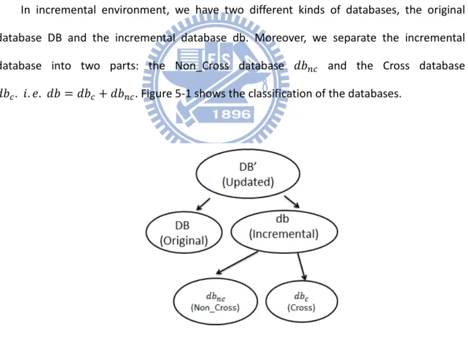
In incremental environment, we have two different kinds of databases, the original database DB and the incremental database db. Moreover, we separate the incremental database into two parts: the Non_Cross database 𝑑𝑏𝑛𝑐 and the Cross database 𝑑𝑏𝑐. 𝑖. 𝑒. 𝑑𝑏 = 𝑑𝑏𝑐+ 𝑑𝑏𝑛𝑐. Figure 5-1 shows the classification of the databases.

Figure 5-1: The classification of the databases.

The Non_Cross database, denoted as 𝑑𝑏𝑛𝑐, is referred to as the set of new instances which have no neighbor instances occurred in DB. The Cross database, denoted as 𝑑𝑏𝑐, is the

25

set of new instances which have neighbor instances existed in DB. Figure 5-2 shows the concepts of Non_Cross database and Cross database in an updated topological spatial temporal database.

Figure 5-2: The concepts of Non_Cross database and Cross database

A database combining all the data instances from DB and db is referred to as the updated database DB’. An extended database EDB is the set of instances from incremental database db and instances in the original database DB which are neighbors of the instances in 𝑑𝑏𝑐. Figure 5-3 shows an example of the extended database EDB.

26

In the extended database EDB, we have to modify the definition of the measurement of discovering frequent topological patterns to avoid losing accurate count information. Different from the prevalence in Eq.(3-4) which determines the minimum participation ratios among all features of a pattern S, we define a new measurement, Max_PV(S) in Eq.(5-1) which determines the maximum participation ratios among all features in a pattern S. If Max_PV (S) < min_prevalence, pattern S is impossible to become frequent.

Max_PV (S) =max { 𝑝𝑟(𝑓𝑖, 𝑆), ∀ 𝑓𝑖 ∈ 𝑆 }. (5-1)

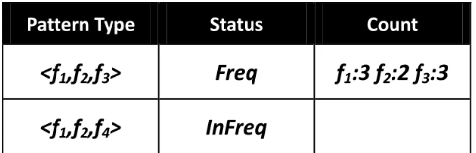
With the intention of incremental maintenance of topological patterns in spatial temporal databases, we need to store important information from the previous results which can be re-used. First, we store Frequent Pattern Set (FPS) which is the set of frequent patterns from the previous mining result. We also store the count information of each frequent pattern in Count Information (CI). There are three columns in Count Information: Pattern Type, Status, and Count. Pattern Type shows the feature types involved in this pattern. Status shows the frequency of this pattern. Count records the counts of each feature in a frequent pattern. Figure 5-4 shows an example of Count Information. In the example, <𝑓1, 𝑓2, 𝑓3> is a frequent pattern, and we mark the Status of < 𝑓1, 𝑓2, 𝑓3 > as Freq. Moreover, we store the counts of each feature 𝑓1: 3, 𝑓2: 2, 𝑓3: 3.

Pattern Type

Status

Count

<f

1

,f

2

,f

3

>

Freq

f

1

:3 f

2

:2 f

3

:3

<f

1

,f

2

,f

4

>

InFreq

27

Problem Statement:Consider a spatial-temporal database DB, the minimum prevalence threshold min_prevalence, a frequent topological pattern set FPS from DB, and an incremental database db. The problem of incremental maintenance of topological pattern is to maintain the set of frequent topological pattern FPS’ in an updated database DB’ based on the information of FPS instead of re-mining DB’ from scratch.

5.2 The Basic Concept of Inc_TMiner

We improve the efficiency of the existing algorithms. Hence, we design a new core algorithm for Inc_TMiner which combines the advantages of Topology Miner and Join-less Collocation Miner.

First, with the intention of incremental maintenance of topological patterns, we need to store the neighborhood relationships among instances. Therefore, we utilize the star neighborhood based on the concept of star neighborhood in Join-less Collocation Miner. It reduces the expensive cost of join operations in discovering topological patterns. Moreover, when we incrementally maintain the discovered topological patterns, we may re-mine the original database to retrieve accurate information in some cases. Instead of re-scanning the original database, we discover patterns from the star neighborhood which is more efficient. Figure 5-5 shows an example of the original database and its star neighborhood.

28

Figure 5-5: An example of (a) the original database (b) star neighborhood.

In order to find neighbor instances efficiently, we design a Cube-Feature Index structure based on the concept of summary structure in Topology Miner. Cube-Feature Index is built with the composite key (<𝑐𝑥𝑖,𝑦𝑖, 𝑤𝑠>,𝑓𝑖), and its first level is used to index the cube with the

identifier <𝑐𝑥𝑖,𝑦𝑖, 𝑤𝑠> and its second level indexes the feature type 𝑓𝑖. With this structure, we

can obtain the feature count occurred in a cube <𝑐𝑥𝑖,𝑦𝑖, 𝑤𝑠>. Moreover, it is easier to discover

the neighbor cubes of <𝑐𝑥𝑖,𝑦𝑖, 𝑤𝑠> and retrieve the neighbor instance counts.

Finally, we generate candidate patterns using lexicographic Pattern-Growth method mentioned in Topology Miner. Pattern-Growth method is one of the most effective methods for frequent pattern mining and superior to candidate-maintenance-test approach. We also make use of Apriori property to prune the impossible candidate patterns.

29

5.3 The Updating Process of Inc_TMiner

In this section, we discuss the updating process of Inc_TMiner. First, we discuss the different cases when the database updated. Second, we give the details of our algorithm with examples.

5.3.1 Cases of Updating Process

When an original database DB is updated to DB’, we have to check the extend database EDB to update frequent patterns in FSP. There are several cases.

Case 1. If pattern S which appears in EDB is frequent in DB, then we update the count

information CI. It is easy to handle since we have already kept the count information from the previous mining result.

Case 2. If pattern S which appears in EDB is not frequent in DB, then we check Max_PV (S) in

EDB. If Max_PV(S) is greater than or equal to min_prevalence, then we re-mine the original database (Case 2.1). On the contrary, if Max_PV(S) ≤ min_prevalence, then it is impossible to become frequent in an updated database (Case 2.2) based on theorem 1.

Theorem 1. If a topological pattern S is not frequent in the original database DB and Max_PV(S) < min_prevalence in EDB, it is impossible to become frequent in an updated database DB’.

Proof: 𝑓𝑚𝑎𝑥 is the feature with max participation ratio in pattern S in EDB.

𝑛𝐷𝐵, 𝑛𝐸𝐷𝐵, 𝑛𝐷𝐵′ are the numbers of 𝑓𝑚𝑎𝑥 which participate in pattern S in DB,EDB,DB’

𝑁𝐷𝐵, 𝑁𝐸𝐷𝐵, 𝑁𝐷𝐵′ are the number of 𝑓𝑚𝑎𝑥 in DB, EDB, DB’.

30 𝑛𝐷𝐵 𝑁𝐷𝐵<min_prevalence 𝑛𝐷𝐵<min_prevlence* 𝑁𝐷𝐵 𝑛𝐷𝐵+𝑛𝐸𝐷𝐵 <min_prevalence* 𝑁𝐷𝐵+𝑛𝐸𝐷𝐵 𝑛𝐷𝐵+𝑛𝐸𝐷𝐵 𝑁𝐷𝐵+𝑁𝐸𝐷𝐵<min_prevalence+𝑛𝐸𝐷𝐵-min_prevalence * 𝑁𝐸𝐷𝐵 𝑛𝐷𝐵′ 𝑁𝐷𝐵′<min_prevalence+𝑛𝐸𝐷𝐵-min_prevalence * 𝑁𝐸𝐷𝐵 If 𝑛𝐸𝐷𝐵-min_prevalence * 𝑁𝐸𝐷𝐵 ≤0, then _𝑁𝑛𝐷𝐵′

𝐷𝐵′ is impossible to be greater than or equal

to min_prevalence. So 𝑛𝐸𝐷𝐵

𝑁𝐸𝐷𝐵≤ min_prev, then pattern S is infrequent in the updated database.

Case 3. If pattern S which does not appear in EDB is frequent in DB, we re-calculate the

prevalence. Since we have already kept the count information, it is easy to compute the prevalence.

5.3.2 Inc_TMiner Algorithm

The Inc_TMiner algorithm has three phases. First, we update the Star Neighborhood and find the extended database in the Update phase. Second, the Star Mining phase discovers star-like patterns and 2 clique-like patterns in the updated database. Finally, the Clique-Mining phase is mining frequent clique-like patterns.

Figure 5-6 shows the framework of Inc_TMiner. It takes the Frequent Pattern Set FSP, the Count Information CI, the Star Neighborhood SN from the previous mining result, and the incremental database db as input. It outputs the set of frequent topological patterns and Figure 5-7 shows the pseudo code of Inc_TMiner. We explain the process of Inc_TMiner with an example step by step.

31

32

33



_{The Update Phase:}

Step I: Update the star neighborhood and determine the extended database EDB (Line 3-Line 4):

First, we update the star neighborhood when inserting the new instances and determine the extended database EDB. Figure 5-8 shows an example of the updated database DB’. We also mark the extended database EDB in this example. A special instance 𝑓1. 𝑒 which is an instance in the original database is also an instance in the extended database, since 𝑓1. 𝑒 is the neighbor of 𝑓3. 𝑒 and 𝑓4. 𝑒.which are instances in the Cross database.

Figure 5-8: An example of the updated database DB’ and the extend database EDB

Through the summary-structure, we discover the neighbor instances of new instances { 𝑓1. 𝑓, 𝑓1. 𝑔, 𝑓2. 𝑒, 𝑓2. 𝑓, 𝑓2. 𝑔, 𝑓2. ℎ, 𝑓2. 𝑖, 𝑓3. 𝑒, 𝑓3. 𝑓, 𝑓3. 𝑔, 𝑓3. ℎ, 𝑓4. 𝑒,

𝑓4. 𝑓} which are inserted into the incremental database. We store these new instances and the neighbor instances of these new instances in star neighborhood. Figure 5-9 is the star

34

neighborhood of the extended database.

Figure 5-9: The star neighborhood of the extended database.



_{The Star Mining Phase}

Step II: Update the count information of 2 clique–like patterns and mine frequent star –like patterns and 2 clique-like patterns. (Line 5-Line 7)

We can obtain the feature counts of 2 clique-like patterns directly from star

neighborhood. Therefore, we update the feature counts of each 2 clique-like patterns in CI since we have already stored the count information from the previous result. For each 2-clique-like pattern, we add the feature counts in extended database to the feature counts in CI.

Figure 5-10 shows the count information after database updated. Take pattern <𝑓1, 𝑓2> as an example, the feature counts of <𝑓1, 𝑓2> in the original database are 𝑓1: 2, 𝑓2: 2 , and the counts in the extended database are 𝑓1: 2 𝑓2: 2. Therefore, the feature counts of <𝑓1, 𝑓2> in the updated database are 𝑓1: 4 𝑓2: 4.

35

Figure 5-10: The count information after database updated

We mine star-like patterns by checking the counts of 2-clique-like patterns in Count Information. We calculate the participation ratio pr (𝑓𝑗, (𝑓𝑖, 𝑓𝑗)) of each related feature 𝑓𝑗 of the center feature 𝑓𝑖, if the participation ratio of the feature 𝑓𝑗 is greater than or equal to min_prevalence, then this feature is one of star features of 𝑓𝑖. Take the center feature 𝑓1 as an example, the participation ratio of each related features which are pr(𝑓2,, <𝑓1,𝑓2>)

=0.44, pr(𝑓3, <𝑓1,𝑓3>) =0.75 and pr(𝑓4,, <𝑓1,𝑓4>) =0.83 are greater than min_prevalence 0.35, the star pattern of 𝑓1 is <𝑓1: 𝑓2, 𝑓3, 𝑓4>.

36

patterns. Figure 5-11 shows an example of mining 2-clique-like patterns, in this example, <𝑓1,𝑓4> is frequent in the original database since the participation ratios are pr(𝑓4,, (𝑓1,𝑓4)) =3/4, pr(𝑓1, (𝑓1,𝑓4)) =2/5 and the prevalence of <𝑓1,𝑓4> is min {2/5, 3/4} = 0.4 which is greater than min_prevalence 0.35.In the updated database, the prevalence of <𝑓1,𝑓4> changes to min {3/7, 5/6} =0.42 since the participation ratios are pr(𝑓4,, <𝑓1,𝑓4>) =5/6, pr(𝑓1, <𝑓1,𝑓4>) =3/7. <𝑓1,𝑓4> is still frequent after database updated.

Figure 5-11: An example of count information after the Star Mining Phase.



_{Clique Mining Phase}

Step III: Extend each frequent 2-clique-like pattern in EDB by the pattern growth method. (Line 8 – Line 11)

As we already know the frequent 2 clique-like patterns in the updated database are {<𝑓1,𝑓2>, <𝑓1,𝑓3>, <𝑓1,𝑓4>, <𝑓2,𝑓3>, <𝑓3,𝑓4>}, we extend each 2-clique-like pattern in EDB by

37

the pattern growth method, and also make the use of Apriori property to prune the impossible candidate patterns. For each extended pattern 𝑆𝑒, we check whether the extended pattern 𝑆𝑒 is in FPS, then we handle the extended pattern 𝑆𝑒 in different cases to determine the pattern is frequent in the updated database.

Step IV: (Case 1) If an extended pattern 𝑺𝒆 is in FPS, then we update the count information of 𝑺𝒆 (Line 1 - Line 2 in the Inc_PDB Procedure)

In this example, we extend the frequent pattern <𝑓1,𝑓2> to <𝑓1,𝑓2,𝑓3>. Because <𝑓1,𝑓2,𝑓3> is already in FPS, we have already stored the count information, the feature counts of <𝑓1,𝑓2,𝑓3> in the updated database is the sum of the feature counts in CIand the feature counts in EDB. Then we calculate the prevalence of <𝑓1,𝑓2,𝑓3> is min {3/7,3/9,3/8} = 0.33 which is less than min_prevalence 0.35 . Hence, <𝑓1,𝑓2,𝑓3> becomes infrequent in the updated database. Figure 5-12 shows the process of determining the frequency of pattern <𝑓1,𝑓2,𝑓3>

38

Step V :( Case 2) If the extended pattern 𝑺𝒆 is not in FPS, we re-mine the original database. (Line 3- Line 4 in the Inc_PDB Procedure)

If an extended pattern 𝑺𝒆 is not in FPS, we did not keep any count information about this pattern, so we have to check the Max_PV (𝑆𝑒) in EDB. In this example, <𝑓1,𝑓3,𝑓4> is not in FPS, and the feature counts of <𝑓1,𝑓3,𝑓4> in EDB are 𝑓1: 2 𝑓3:2 𝑓4: 2. The Max_PV (<𝑓1,𝑓3,𝑓4>) is max {2/2, 2/4, 2/2} =1 which is greater than min_prevalence 0.35. It meets the condition of case 2.1. Therefore, we re-mine the original database, we obtain the feature counts in DB as 𝑓1: 1 𝑓3:1 𝑓4: 1. Then sum the counts in EDB and in DB, we obtain the feature counts in DB’ 𝑓1: 3 𝑓3:3 𝑓4: 3. Finally we calculate the prevalence of <𝑓1,𝑓3,𝑓4> is min {3/7,3/8,3/6} = 0.375 ≥ 0.35. We determine <𝑓1,𝑓3,𝑓4> is a frequent pattern after database updated. Figure 5-13 shows the process of determining the frequency of pattern <𝑓1,𝑓3,𝑓4>.

39

Step VI: (Case 3) for each pattern S is in FPS, but not appears in EDB, we re-calculate the prevalence. (Line 13 – Line 15)

The topological pattern S does not appear in EDB, but S is frequent in DB, then it is possible to become frequent in DB’. We check the prevalence due to the change of the number of 𝑓𝑖 in the updated database. In this example, <𝑓2, 𝑓3, 𝑓4> does not appear in EDB, but it is a frequent pattern in FPS, so we re-calculate the prevalence. The prevalence of <𝑓2, 𝑓3, 𝑓4> in DB is min {2/5, 2/4, 2/4} =0.4, and changes to min {2/9, 2/8,2/6}=0.22 in DB’. <𝑓2, 𝑓3, 𝑓4> becomes infrequent after database updated. Figure 5-14 shows the process of determining the frequency of pattern <𝑓2,𝑓3,𝑓4>

Figure 5-14: The process of determining the frequency of pattern <𝒇_𝟐,𝒇_𝟑,𝒇_𝟒>

Finally, we discover that the frequent patterns in the updated database are {<𝑓1,𝑓2>, <𝑓1,𝑓3>, <𝑓1,𝑓4>, <𝑓2,𝑓3>, <𝑓3,𝑓4>,<𝑓1,𝑓3,𝑓4>}. Figure 5-15 shows the flowchart of

40

41

Chapter 6. Experimental results and performance study

To evaluate the performance of Inc_TMiner, two topological pattern mining algorithms based on static databases, Topology Miner [7], Join-less Colocation Miner [5], and one incremental spatial-temporal topological pattern maintaining algorithm IMCP based on Join-less Colocation Miner method are implemented for comparison. All algorithms are implemented in C++ language and tested on an Intel Centrino 1.3 GHz U7300 with 2 GB of main memory running Windows 7 system. We test the performance on synthetic databases with different parameters setting.

42

6.1 Data Generator

Figure 6-1: Parameters of synthetic data generator

We extend the synthetic data generator used for mining topological pattern in static spatial-temporal databases [7]. Figure 6-1 shows the parameters setting of incremental spatial-temporal data generator.

43

In our experiments, we set N as the number of instances in an incremental spatial temporal database. Incre_Ratio divides the spatial-temporal database into two parts, the original database and the incremental database. N*(1-Incre_Ratio) is the size of the original database DB and N*Incre_Ratio is the size of the incremental database db. Moreover, we divide the incremental database into the Non-Cross database and the Cross database by Cross Ratio. The size of Non_Cross database is N*Incre_Ratio*(1-Cross_Ratio), and the size of the Cross database is N*Incre_Ratio*Cross_Ratio.

In each database we divide the instances by several parameters. First, we set L as the number of features which appear in the longest pattern and m is the number of features which are confident in the longest pattern. The confident features should participate in the frequent patterns. n is the number of noise features, and H is the percentage of noise instances in the database. N*(1-Incre_Ratio)*H is the number of noise instances in the original database. We assign these instances to noise features uniformly. The rest of instances are assigned to non-noise features uniformly. Θ is min_prevalence. (Δmax +Θ) is the percentage of confident instances which appear in the longest pattern. The number of instances 𝑁𝑖, which must appear in the longest pattern of a feature 𝑓𝑖 in the original database is (Δmax +Θ)* N*(1-Incre_Ratio)*(1-H) /L. For other features, the participation ratio is (Δmin +Θ) and the number of instances in the longest pattern in the original database is (Δmin +Θ)* N*(1-Incre_Ratio)*(1-H) /L.

We divide the spatial-temporal space by the cube-size with the spatial distance value _2√2𝑅 and temporal distance value 𝑇_𝑢𝑛𝑖𝑡𝑠₂ . First, we generate a center instances (𝑥𝑐, 𝑦𝑐, 𝑡𝑐) randomly, then we generate the instances around a circle with a radius r. the location coordinate is (𝑥_𝑐 + 𝑟 ∗ sin2𝜋

𝑁𝑖, 𝑦𝑐+ 𝑟 ∗ cos

2𝜋

𝑁𝑖), the temporal coordinate is 𝑡𝑐+ 𝑇_𝑢𝑛𝑖𝑡 ∗ sincos

2𝜋 𝑁𝑖 . We

confirm all instances in the cube will participate in the longest pattern. We mark the cubes which intersect the cylinder. The centered of circle of cylinder is radius r and the height of

44

the cylinder is 2*T_unit. No other longest pattern instance can generate in this circle. After generating instances of each feature which participate in the frequent pattern, the process is end. We generate the remaining instances randomly on the space.

6.2 Performance

In this section, we discuss the performance of Inc_TMiner. As to the comparison of Inc_TMiner, we implement the other three algorithms, Topology Miner and Join-less Collocation Miner and IMCP.

With the intention to show the efficiency of Inc_TMiner, we vary Cross_Ratio, Incre_Ratio and prevalence threshold to measure the execution times and memory usage of the four algorithms. We also show scalability of Inc_TMiner by vary the data size of the spatial temporal databases.

6.2.1 Effect of Cross Ratio

We study the performance of the four algorithms by varying Cross_Ratio from 0.05 to 0.5. Figure 6-2 shows the effect of Cross_Ratio of the four algorithms v.s. the execution times. When Cross_Ratio increases, the number of instances in the cross database also increases. The execution times of the four algorithms also increase since more computations are required for higher interaction relations between the original database and the incremental database. However, Inc_TMiner still outperforms other algorithms and has a better performance when Cross_Ratio is small.

45

Figure 6-2: The effect of Cross Ratio

6.2.2 Effect of Incre Ratio

We evaluate the performance of the four algorithms by varying the Inc_Ratio from 0.05 to 0.5. The results of the four algorithms shown in Figure 6-3 indicate Inc_TMiner outperforms the other three algorithms. When the Inc_Ratio increases, the number of instances in the incremental database also increases, the four algorithms require more time to discover topological patterns. When Inc_Ratio is in lower value, both the incremental algorithms require less time compared to the static algorithms, since the size of the incremental database in the updated database is smaller. The experiment shows Inc_TMiner is more efficient than the other three algorithms, especially in small Inc_Ratio.

46

Figure 6-3: The effect of Incre Ratio

6.2.3 Effect of Data Size

We study the effect of the number of instances N in the updated database. Figure 6-4 shows the results of the four algorithms with varing the number of instances from 100k to 1000k. Figure 6-5 depicts the performance of two incremental algorithms. Both incremetal miners significantly outperform the static algorithms, especially when the number of instances is greater than 500k, since the static algorithms reqiure to re-mine the updated databases which are much larger than the incremental databases. When the number of instances increases, Inc_TMiner requires less time to discover topological patterns compared to the other three algorithms. Moreover, Inc_TMiner outperforms IMCP, since Inc_TMiner discovers frequent topological patterns in the depth-first method and maintains the corresponding projected databases. Figure 6-6 shows the effect of data size versus memory usage. When data size increases, the memory usage also increases. Incremental algorithms are less effective than static algorithms because the incremetnal algorithms require to keep some extra information count information, frequent pattern set to efficiently maintain

47

topological patterns. Moreover, both Inc_TMiner and Topology Miner use the projected database to facilitate the mining performance which also require extra memory storage.

Figure 6-4: The effect of Data Size v.s. Runtime

48

Figure 6-6: The effect of Data Size v.s. Memory Usage

6.2.4 Effect of Prevalence Threshold

Finally, we test the performance of min_prevalence by varying the value from 0.01 to 0.3. Figure 6-7 shows the performance of the four algorithms. When the min_prevalence increases, the execution times of the four algorithms decreases as expected since when the prevalence threshold increases, more topological patterns become infrequent. As a result, both static algorithms require more time to discover topological patterns than the incremental algorithms. Moreover, in the comparison of two incremental algorithms, Inc_TMiner takes less time than IMCP which is based on the candidate-maintenance-test method. Figure 6-8 shows the memory usage of the four algorithms. When min_prevalence increases, the memory usages of the four algorithms decrease since more topological patterns become infrequent.

49

Figure 6-7: The effect of min_prevalence V.S. Runtime

50

Chapter 7. Conclusion

In this thesis, we investigate the issues for incremental maintenance of topological patterns in large spatial temporal databases. We propose an efficient algorithm Inc_TMiner by exploring techniques to maintain discovered topological patterns in spatial-temporal databases in an incremental environment.

We improve the efficiency of the existing static algorithms, Topology Miner and Join-less Collocation Miner. We use Cube-Feature Index as a summary structure which is efficient to determine the neighbor relationships among instances and approximate the feature count in a cube. With the intention of storing the neighbor relationship we obtain from Cube-Feature Index structure, we utilize star neighborhood which materializes the neighbor set of each instance. Instead of re-scanning the original databases and re-find the neighbor relationship among instance, we retrieve the neighbor set of an instances from star neighborhood. For incremental maintenance of topological patterns, we store the previous mining results which can be re-used. We store frequent patterns in FPS and record the feature counts of the frequent patterns in count information CI.

Inc_TMiner discovers patterns in the Pattern-Growth method which is superior to the candidate-maintenance–test approach. Moreover, it utilizes the concept of the projected database which partitions the databases into subset recursively. It also makes use of the Apriori property to prune the impossible candidate patterns.

Inc_TMiner efficiently maintain topological patterns in incremental environment without re-mining the updated database. Compared to the existing incremental algorithm IMCP and the prior static algorithms Topology Miner and Join-less Collocation Miner, the experiments show that the Inc_TMiner is efficient and scalable compared with than the other three algorithms.

51

Bibliography

[1] R. Agrawal and R. Srikant, “Fast algorithms for mining association rules,” Proc. of the 20th International Conference on Very Large Data Bases (VLDB), Santiago, pp.487-499, 1994.

[2] J. S. Yoo, S. Shekhar, and M. Celik, “A join-less approach for co-location pattern mining: A summary of results,” Proc. of the 5th IEEE International Conference on Data Mining (ICDM), Houston, Texas, pp. 813–816, 2005.

[3] S. Shekhar and Y. Huang, “Discovering spatial co-location patterns: A summary of results,” Proc. of the 7th International Symposium on Spatial and Temporal Databases (SSTD '01), Redondo Beach, CA, pp. 236-256, July 2001.

[4] J. Yoo, S. Shekhar, J. Smith, and J. Kumquat, “A partial join approach for mining co-location patterns,” Proc. of the 12th annual ACM international workshop on Geographic information systems, Washington D.C., USA, pp. 241–249, 2004.

[5] J. Yoo and S. Shekhar, “A join-less approach for mining spatial colocation patterns,” IEEE Trans. on Knowledge and Data Engineering, vol. 18, no. 10, pp.1323-1337, Oct. 2006.

[6] X. Zhang, N. Mamoulis, D. W. Cheung, and Y. Shou, “Fast mining of spatial collocations,” Proc. of the 10th ACM SIGKDD Int'l Conf. Knowledge Discovery and Data Mining (KDD '04), pp. 384-393, 2004.

[7] J. Wang, W. Hsu, and M. L. Lee, “A Framework for Mining Topological Patterns in Spatio-temporal Databases,” Proc. of 14th ACM Conference on Information and Knowledge Management (CIKM '05), Bremen, Germany, pp. 429-436, Nov 2005.

[8] D. Cheung, J. Han, V. Ng, and C.Wong, “Maintenance of discovered association rules in large databases: An incremental updating technique,” Proc. of the 12th International Conference on Data Engineering (ICDE), pp. 106–114, 1996.

[9] J. He, Q. He, F. Qian, and Q. Chen, “Incremental Maintenance of Discovered Spatial Colocation Patterns,” Workshops Proc. of the 8th IEEE International Conference on Data Mining (ICDM '08), Pisa, Italy, pp. 399-407, December 2008.

[10] J. Wang, W. Hsu, M. L. Lee, and J. Wang, “FlowMiner: Finding Flow Patterns in Spatio-Temporal Databases,” Proc. of 16th IEEE International Conference on Tools with Artificial Intelligence (ICTAI '04), Boca Raton, Florida, pp. 14-21, November 2004. [11] J. Wang, W. Hsu, and M. L. Lee, “Mining Generalized Spatio-Temporal Patterns,” Proc.

of 10th International Conference on Database Systems for Advanced Applications (DASFAA), Beijing, China, pp. 649-661, April 2005.