在全基因關聯分析中利用總體的基因表現量作為穩定表現型

國 立 交 通 大 學

統計學研究所

碩 士 論 文

在全基因關聯分析中

利用總體的基因表現量作為穩定表現型

Using Global Gene Expression as Endophenotypes

in a Genome-wide Association Study

研 究 生：蔡佩芳

指導教授：黃冠華 博士

在全基因關聯分析中

利用總體的基因表現量作為穩定表現型

Using Global Gene Expression as Endophenotypes

in a Genome-wide Association Study

研 究 生：蔡佩芳 Student: Pei-Fang Tsai

指導教授：黃冠華 Advisor: Dr. Guan-Hua Huang

國 立 交 通 大 學

統計學研究所

碩 士 論 文

A Thesis

Submitted to institute of Statistics College of Science

National Chiao Tung University in Partial Fulfillment of the Requirements

for the Degree of Master

in Statistics July 2008

Hsinchu, Taiwan, Republic of China

中華民國九十七年七月

在全基因關聯分析中

利用總體的基因表現量作為穩定表現型

研究生：蔡佩芳 指導教授：黃冠華 博士

國立交通大學統計學研究所

摘要

在生物學上，穩定表現型(endophenotype)和疾病有著相同的遺傳路徑，但 穩定表現型卻比診斷上的表現型(phenotype)更為接近其相關的基因，這也顯示 穩定表現型在複雜疾病上基因研究的重要性。穩定表現型為主的基因遺傳分析比 表現型為主的基因遺傳分析更容易找到致病基因。由穩定表現型所發展的指標 (PHE)，穩定表現型的基因遺傳性所佔比例，用在判別出有可能的穩定表現型。 在這篇報告裡，氣喘是一種基因間作用和環境因素複雜的疾病，我們利用基 因表現量當作穩定表現型找尋可能的氣喘基因。我們利用指標(PHE)判斷哪些探 針組的基因表現量是穩定表現型，接著作指標(PHE)的檢定。針對多重檢定的問 題，我們利用 q-值來控制錯誤發現率和調整。我們也對每一個基因表現量做全 基因關聯分析，比較基因表現量指標(PHE)中有顯著和沒有顯著之間基因遺傳性 的變化。最後，我們論文中有(1) 評估利用基因表現量當作穩定表現型找尋跟疾 病有相關基因的適當性，(2) 檢驗從基因表現量為主的分析，辨別出的基因和文 獻中提過疾病相關的基因重複的多寡，(3) 從這些基因表現量判定為穩定表現型 中，評估它們基因遺傳的特徵。 關鍵字: 順式作用 (cis effect) ; 穩定表現型 ; 表現量位置 ; 全基因關聯分

Using Global Gene Expression as Endophenotypes

in a Genome-wide Association Study

Student: Pei-Fang Tsai Advisor: Dr. Guan-Hua Huang

Institute of Statistics

National Chiao Tung University

ABSTRACT

Endophenotype, which involve the same biological pathways as diseases but

presumably are closer to the relevant gene action than diagnostic phenotypes, have

emerged as an important concept in the genetic studies of complex diseases.

Endophenotype-based genetic analysis is more likely to succeed than

phenotype-based one in terms of search for the susceptibility genes. The index,

proportion of heritability explained (PHE), has been proven useful in identifying

potential endophenotypes.

In this report, we use global gene expression as endophenotypes in search for the

susceptibility genes underlying asthma, which is a disease caused by complex

interactions of genetic and environmental factors. We judge which gene expressions

of probe sets are endophenotypes by using the index PHE and do hypothesis test of

PHE. For the problem of multiple testing, we utilize the q-value to control for the

false discovery rate (FDR) for significance judgment. We also perform genome-wide

association tests for each gene expression and compare various genetic properties

between gene expressions with and without significant PHE values. At the end, this

thesis has (1) evaluated the appropriateness of using global gene expressing as

overlap between genes identified by the gene-expression-based analysis and genes

already identified in the literature, and (3) assessed genetic characteristics of gene

expressions that are identified as the endophenotypes.

Key words: Cis effect ; Endophenotype ; Expression quantitative trait loci ;

誌 謝

這兩年來，首先感謝老師 黃冠華的指導，常常因為一點小問題就跑去找老 師，老師都很熱心地幫忙解決問題和疑惑。最後還讓老師非常頭痛地改我的論 文，對老師感到非常不好意思。也感謝老師一年來的訓練，學到很多看書和抓重 點的技巧，也學習到面對一個全新領域一開始應有的應對方式，這一年來獲益良 多。最後對老師在說一聲 謝謝。也感謝其他老師的教導，讓我對統計更有了解。 接下來要感謝我的同學們，像是同老師的同學們 重耕、彥銘和仲竹，彼此間 會互相幫忙指導和提醒對方事情。另外也感謝夙吟、姿蒨、郃嵐和瑜達聽我練習 和給我意見。也非常感謝其他的同學們，因為有你們讓我的研究所生活很精彩。 最後感謝我的家人，常常給我鼓勵和指導一些論文的事項，謝謝你們! 在此，謹以此篇論文，獻給我親愛的家人和同學，還有陪伴我的好朋友們! 蔡佩芳 2008.07.02

Contents

摘要... I 

ABSTRACT ...II 

1  INTRODUCTION...1 

2   LITERATURE REVIEW...4 

2.1   STATISTICAL VALIDATION OF SURROGATE ENDPOINTS...4 

2.2  STATISTICAL VALIDATION OF ENDOPHENOTYPE...5 

2.2.1  Model...6  2.2.2  Variance ofPHE ...10  2.2.3  The covariance of * * ( ) ( ) ˆt _and ˆt q _q h h ... 11  2.2.4  Hypothesis test ...14 

2.3  THE WHOLE-GENOME ASSOCIATION TEST FOR QUANTITATIVE OUTCOMES...14 

2.4  THE PREPROCESSING METHOD FOR GENE EXPRESSION LEVELS...16 

2.4.1  Background adjustment...16 

2.4.2  Normalization ...16 

2.4.3  Summarization ...16 

2.4.4  RMA ...16 

2.5  THE DIFFERENTIAL EXPRESSION METHODS...18 

2.5.1  Fold-change ...18 

2.5.2  Two sample t-test...18 

2.5.3  SAM (Significance Analysis of Microarrays) ...19 

2.6   MULTIPLE TESTING PROCEDURES...20 

2.6.1  Type I error rates...21 

2.6.2  Adjusted p-values ...22 

2.6.3  The q-value...23 

2.7  DATASETS...24 

3  MATERIALS AND METHODS ...26 

3.1  DATASETS...27 

3.2  STATISTICAL METHOD OF ENDOPHENOTYPE...27 

3.3  THE PREPROCESSING AND DIFFERENTIAL METHOD...29 

3.4  GENOME-WIDE ASSOCIATION TESTS FOR GENE EXPRESSIONS...30 

3.5   ASTHMA GENES AND OVERLAP RATE...30 

3.6.2  The scatter plot of heritability of gene expressions versus PHEs...32 

3.6.3...The bar-plot of proportions of probe sets with max significant SNPs’ LOD >6 versus PHEs………32 

3.6.4 The bar-plot of number of cis eSNPs <100 kb or cis eSNPs >100 kb or trans versus PHEs...………33 

3.6.5  The bar-plot of number of cis eSNPs <100 kb or cis eSNPs >100 kb or trans versus heritability of gene expressions and differential expressions. ...34 

3.6.6  The density plot of LOD score for cis eSNPs <100 kb, cis eSNPs >100 kb and trans ...36 

4  RESULT...37 

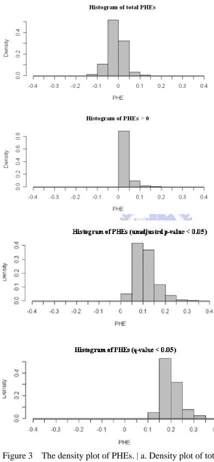
4.1  TEST OF PHES AND THE DISTRIBUTION OF DIFFERENT CONDITIONS OF PHES...37 

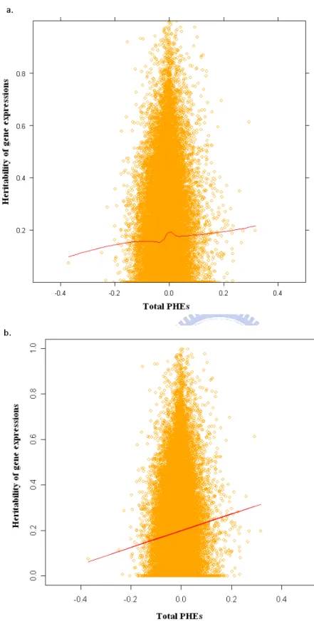
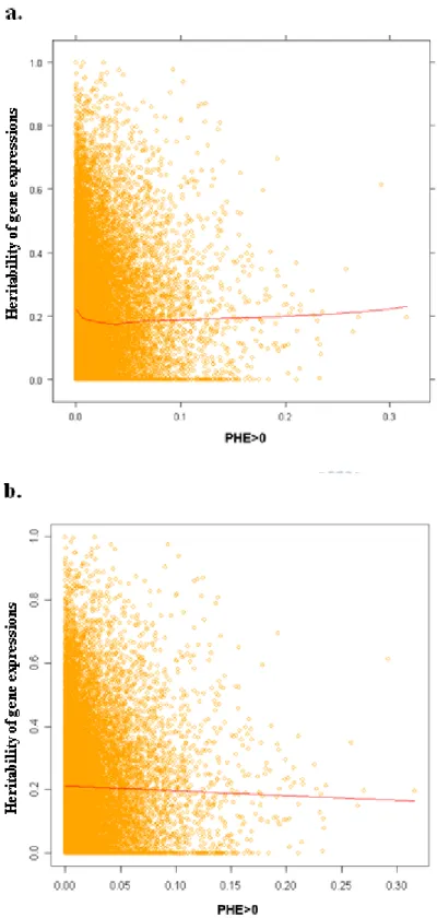
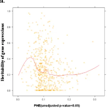
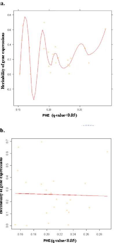
4.2   THE SCATTER PLOT OF HERITABILITY OF GENE EXPRESSION VERSUS PHES...37 

4.3  THE OVERLAP RATE...38 

4.4  THE RESULT OF ASSOCIATION TEST UNDER FOUR CONDITIONS OF PHES...39 

4.4.1  The bar-plot of proportion of probe sets with max significant SNPs’ LOD >6 versus PHEs 39  4.4.2  The bar-plot of the number of cis eSNPs <100 kb or cis eSNPs >100 kb or trans versus PHEs 40  4.4.3  The bar-plot of number of cis eSNPs <100 kb or cis eSNPs >100 kb or trans versus heritability of gene expressions and differential expressions. ...41 

4.4.4  The density plot of LOD score for cis eSNPs <100 kb, cis eSNPs >100 kb and trans ...42 

5  CONCLUSIONS AND DISCUSSION...43 

5.1  CONCLUSIONS...43 

5.2  DISCUSSION...44 

REFERENCE ...45 

APPENDIX I...74 

Figures and Tables Content

FIGURE 1 A SURROGATE ENDPOINT VERSUS AN ENDOPHENOTYPE IN THE DISEASE PROCESS...48 

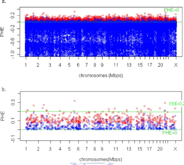
FIGURE 2 THE CONFIDENCE INTERVAL OF PHES ON ALL CHROMOSOMES (RED:PHE, BLUE: THE LOW BOUND OF PHE). ...49 

FIGURE 3 THE DENSITY PLOT OF PHES...50 

FIGURE 4 THE SCATTER PLOT OF HERITABILITY VERSUS TOTAL PHES. ...51 

FIGURE 5 THE SCATTER PLOT OF HERITABILITY VERSUS PHES >0...52 

FIGURE 6 THE SCATTER PLOT OF HERITABILITY VERSUS PHES WITH UNADJUSTED P-VALUE <0.05. ...53 

FIGURE 7 THE SCATTER PLOT OF HERITABILITY VERSUS PHES WITH Q-VALUE <0.05. ...54 

FIGURE 8 THE BAR-PLOT OF PROPORTION OF PROBE SETS WITH MAX SIGNIFICANT SNPS’LOD>6 VERSUS PHES. ...55 

FIGURE 9 THE BAR-PLOT OF THE NUMBER (CIS ESNPS <100KB) VERSUS PHES. ...56 

FIGURE 10 THE BAR-PLOT OF THE NUMBER (CIS ESNPS >100KB) VERSUS PHES. ...57 

FIGURE 11 THE BAR-PLOT OF THE NUMBER (TRANS) VERSUS PHES. ...58 

FIGURE 12 THE BAR-PLOT OF THE NUMBER (CIS ESNPS <100 KB) VERSUS HERITABILITY AND DIFFERENTIAL EXPRESSION. ...59 

FIGURE 13 THE BAR-PLOT OF THE NUMBER (CIS ESNPS >100 KB) VERSUS HERITABILITY AND DIFFERENTIAL EXPRESSION. ...60 

FIGURE 14 THE BAR-PLOT OF THE NUMBER (TRANS) VERSUS HERITABILITY AND DIFFERENTIAL EXPRESSION. ...61 

FIGURE 15 THE DENSITY PLOT OF LOD SCORE FOR CIS ESNPS <100 KB (RED), CIS ESNPS >100 KB (GREEN) AND TRANS (TRANS) BETWEEN X-LIMIT (3,50) AND Y-LIMIT (0,0.8) FOR PROBE SETS WITH TOTAL PHES. ...62 

FIGURE 16 THE DENSITY PLOT OF LOD SCORE FOR CIS ESNPS <100 KB (RED), CIS ESNPS >100 KB (GREEN) AND TRANS (BLUE) BETWEEN X-LIMIT (3,25) AND Y-LIMIT (0,0.3) FOR PROBE SETS WITH TOTAL PHES. ...63 

FIGURE 17 THE DENSITY PLOT OF LOD SCORE FOR CIS ESNPS <100 KB (RED), CIS ESNPS >100 KB (GREEN) AND TRANS (BLUE) BETWEEN X-LIMIT (3,50) AND Y-LIMIT (0,0.8) FOR PROBE SETS WITH PHES>0. ...64 

FIGURE 18 THE DENSITY PLOT OF LOD SCORE FOR CIS ESNPS <100 KB (RED), CIS ESNPS >100 KB (BLUE) AND TRANS (BLUE) BETWEEN X-LIMIT (3,25) AND Y-LIMIT (0,0.5) FOR PROBE SETS WITH PHES>0...65 

FIGURE 19 THE DENSITY PLOT OF LOD SCORE FOR CIS ESNPS <100 KB (RED), CIS ESNPS >100 KB (GREEN) AND TRANS (BLUE) BETWEEN X-LIMIT (3,50) AND Y-LIMIT (0,0.8) FOR PROBE SETS WITH PHES WITH UNADJUSTED P-VALUE <0.05. ...66  FIGURE 20 THE DENSITY PLOT OF LOD SCORE FOR CIS ESNPS <100 KB (RED), CIS ESNPS >100 KB

WITH UNADJUSTED P-VALUE <0.05. ...67 

FIGURE 21 THE DENSITY PLOT OF LOD SCORE FOR CIS ESNPS <100 KB (RED), CIS ESNPS >100 KB (GREEN) AND TRANS (BLUE) BETWEEN X-LIMIT (3,10) AND Y-LIMIT (0,0.8) FOR PROBE SETS WITH PHES WITH Q-VALUE <0.05. ...68 

TABLE 1 GENETIC COMPONENTS OF VARIANCE ASSUMING RANDOM MATING...8 

TABLE 2 THE DERIVATIVE OF COVARIANCE COMPONENTS FOR RELATIVE PAIRS...12 

TABLE 3 PROBABILITY OF CALLING 1 OR MORE FALSE POSITIVES BY CHANCE. ...21 

TABLE 4 TYPE I AND TYPE II ERRORS IN MULTIPLE HYPOTHESIS TESTING. ...21 

TABLE 5 THE PHES OF PROBE SETS WITH Q-VALUE <0.05. ...69 

TABLE 6 THE PROBE SETS WITH PHES >0.2...71 

TABLE 7 GENES OF SIGNIFICANT SNPS (LOD>6) OVERLAP WITH ASTHMA OR ATOPY GENES...72 

TABLE 8 THE PROBE SET WITH MAX ESNPS'LOD>6(PHES WITH Q-VALUE <0.05)...73 

TABLE 9 CIS ESNPS <100 KB (PHES WITH Q-VALUE <0.05). ...73 

1 Introduction

In diseases with classic or Mendelian genetics as their distal causes, genotypes are

usually indicative of phenotypes. However, this degree of genetic certainty does not

exist for complex disease [1]. These “complex” diseases are influenced by multiple

genes, environmental factors and their interactions on phenotypes. As a result, the

direct relationship between phenotype and genotype is disrupted, so that the same

genotype may result in different phenotypes, or different genotypes may result in the

same phenotype. To facilitate the identification of influential genetic markers of

complex disease, endophenotype approach has been advocated.

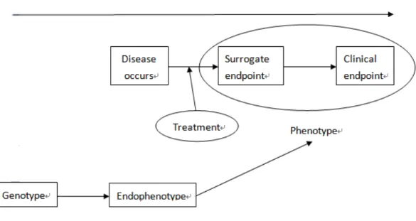
Endophenotypes are useful for theorizing about clinical phenotypes and mark the

path between genotype and phenotype. The endophenotype is closer to the underlying

gene than the phenotype in the course of disease’s natural history and can increase the

chance of identifying genotype (Figure 1). Huang et al. [2] defined an endophenotype

to be “a trait for which a test of null hypothesis of no genetic heritability implies the

corresponding null hypothesis based on the phenotype of interest” and develop a

formal statistical methodology for accessing the utility of endophenotypes, motivated

by the conditioning strategy used for identifying surrogate endpoints in clinical

research. The methodology is especially useful for the situation where underlying

genotype is unknown and researchers use endophenotypes to increase opportunities of

finding susceptible disease genes. Similar to validating surrogate endpoints, various

indices can be used to validate endophenotypes. One of the indices is the proportion

of heritability explained (PHE) by the endophenotype, similar to PTE _introduced

by Freedman et al. [3] in the surrogate endpoint study. The greater the PHE value, the

more likely the intermediate variable is an endophenotype. Hsieh et al. [4] utilized the

There is a problem about signal-SNP association test between SNP genotypes and

case-control status: it cannot discover SNPs that are weakly related to the disease by

itself, but can have great impacts on the disease variability after combining with other

SNPs. A large PHE value represents that endophenotype and phenotype share many

genes. Because endophenotype is closer to genotype, there will be some genes that are

significant in endophenotype, but are not significant in phenotype. We can utilize the

PHE to find SNPs that may be weakly associated to the disease phenotype. Hopefully,

these additional SNPs can increase our chances in searching possible

phenotype-related genes.

Gene expression is a measurement of mRNA and mRNA is transcribed from a

DNA template and carries coding information to the sites of protein synthesis.

Because mRNA is closer to DNA genotype, we use global gene expression as

endophenotypes in search for the susceptibility genes underlying asthma, which is a

disease caused by complex interactions of genetic and environmental factor. In this

thesis, we first get global gene expressions of probe sets in Epstein-Barr virus

Iymphoblastoid cell lines (EBVL) measured with Affymetrix HG-U133 Plus 2.0 chip

[5-6]. Gene expression values are preprocessed by the robust multi-array averaging

(RMA). We judge which gene expressions of probe sets are endophenotypes by using

the index PHE and do hypothesis test of PHE. For the problem of multiple testing, we

utilize the q-value to control for the false discovery rate (FDR) for significance

judgment. We also perform genome-wide association tests for each gene expression

and compare various genetic properties between gene expressions with and without

significant PHE values.

Therefore, this thesis aims at

(1) Evaluating the appropriateness of using global gene expressing as

(2) Examining the overlap between genes identified by the gene-expression-based

analysis and genes already identified in the literature, and

(3) Assessing genetic characteristics of gene expressions that are identified as the

2 Literature Review

2.1 Statistical validation of surrogate endpoints

Surrogate endpoints have been frequently utilized in most clinical research, when

the primary endpoint is too difficult or costly or time-consuming to obtain. Clinically

meaningful biomarkers of the disease projected as a surrogate endpoint in a clinical

trial is expected to ultimately demonstrate treatment effect on the primary endpoint if

a treatment effect shown on the markers. Surrogate endpoints have been of clinical

interest for decades, but it was not until Prentice published a seminal paper in 1989

that formal statistical investigation started. Prentice defined a surrogate endpoint to be

“a response variable for which a test of null hypothesis of no relationship to the

treatment groups under comparison is also a valid test of the corresponding null

hypothesis based on the true (clinical) endpoint”.

Prentice’s definition can be written as

( | ) ( ) ( | ) ( )

f S X = f S ⇔ f T X = f T

Where T denotes the status of a primary endpoint, S denotes the status of a

surrogate end-point, X is the treatment variable, f(S) is the distribution of S, and f(S|X)

is the conditional distribution of S given X. Validation of Prentice’s definition

involves the following two criteria:

( | ) ( ) and ( | , ) ( | )

f T S ≠ f T f T S X = f T S

[3, 7-8]. The first criterion states that the surrogate endpoint must be correlated with

the primary clinical endpoint, and the second criterion is that the surrogate endpoint

should fully capture the treatment effect on the treatment effect on the primary

endpoint.

The surrogate endpoint described by Prentice mediates all of the effect of treatment

on the primary endpoint, that is

A more complex, but more likely, situation arises when treatment has a direct effect

on the primary endpoint that is not mediated through the surrogate [9]:

X → →S T

Freedman et al. [3] proposed to focus on the proportion of the treatment effect

mediated through the surrogate. A good surrogate is one that explains large proportion

of that effect. The proposal can be made in the content of generalized linear models

[10]. The net effect of X on T can be assessed through the regression coefficient

T

β in the generalized linear model

[ ( )] _{T T}

g E T =α +β X

Where g(.) is the link function connecting the mean response and covariates, and

the effect of X on T after inclusion of S is the regression coefficient β_TSin the following generalized linear model

[ ( )] _{TS TS TS}

g E T =α +β X+γ S

The proportion of the treatment effect (on the primary endpoint) explain (PTE) by

the surrogate is given by

1 TS

T

PTE β

β = −

The 100(1−α)% confidence limits of PTE can be calculated using the delta method.

2.2 Statistical validation of endophenotype Notation:

1,...,

i= I : representing the different family

1,..., _i

j= n : representing the jth member of this family

2

A

σ : The variances arising from polygenic additive effects, 2

D

σ : The variance arising from polygenic dominance effects 2

C

σ : The variance arising from the shared environmental effects

2.2.1 Model

Endophenotypes are useful for theorizing about clinical phenotypes and can mark

the path between the genotype and the phenotype. Verification of existence of the

pathway genotype-endophenotype-phenotype is the key of validating endophenotypes.

Analogous to Prentice’s definition [7] that surrogate endpoint to be “a response

variable for which a test of null hypothesis of no relationship to the treatment groups

under comparison is also a valid test of the corresponding null hypothesis based on

the true (clinical) endpoint”, Huang et al. [2] define an endophenotype to be “a trait

for which a test of null hypothesis of no genetic heritability implies the corresponding

null hypothesis based on the phenotype of interest”. More specifically, suppose P is

the phenotype of interest, E is the selected endophenotype, and G represents an underlying genetic structure that fulfills the specified assumptions in calculating

heritability, then the proposed definition is:

( | ) ( ) ( | ) ( )

f E G = f E ⇒ f P G = f P (1) The endophenotype’s definition has two important features [2]. First, “imply” replaces

‘’if and only if’’ statement in Prentice’s definition of surrogate endpoints in avoidance

of a problematic implication arisen in Begg and Leung [11]. This change places

endophenotype in higher upstream of the pathway from genotype to phenotype.

Second, genetic heritability represents the proportion of variability attributable to

genetic factors and can be obtained in a variance component approach [12-13]. This is

genes and allows the likelihood of multiple gene influences.

Suppose the condition

( | , ) ( | )

f P E G = f P E (2)

Huang et al. [2] takes (2) in a variance component model as the operational

criterion for proposed endophenotype definition. It then requires heritability of

phenotype becomes null, conditioning on candidate endophenotype, and implies

genetic heritability of phenotype is captured by endophenotype.

Given an observed phenotype, significance of (2) can be judged through the

following variance component analysis for discrete trait [2, 14]:

2 2 2 2 2 2 2 , , , , (0, ) (0,[ ]) (3) cov( , ) 2 , ij H H ij H ij ij ij ij R ij A D C ij ik ij ik A ij ik D ij ik C P E x G Normal G Normal G G j k α γ τ ε ε σ σ σ σ φ σ σ λ σ = + + + + + + = + Δ + ≠ ∼ ∼

(4) Where α_H is a baseline mean, E_ij is his/her corresponding specified endophenotype. The termε_ijis the residual error term representing the effect of non-family factors. The term G is the random effect for the underlying genetic _ij

structure. The term φ_{ij ik,} denotes the kinship coefficient between individual and ij ik : the probability of randomly drawing a single allele in individual ij that is identical by descent (ibd) to a single allele at the same locus

randomly drawn from individualik. The termΔ is the probability that both _{ij ik,} alleles at a locus are shared ibd by individuals ij and .ik the elements,λ_{ij ik,} , is

simply binary indicator denoting whether two individuals live together (λ_{ij ik,} =1 ) or apart (λ_{ij ik,} =0 ).

The (broad sense) heritability ofP , conditional on _ij E is _ij

2 2 2 2 2 2 A D A D C R h σ σ σ σ σ σ + = + + + (4) The significance of rejecting the hypothesis h=0 indicates the fulfillment of (2).

Table 1 details the term φ_{ij ik,} andΔ values for selected relative pairs and the total _{ij ik,} genetic variances that these imply [15].

Table 1 Genetic components of variance assuming random mating.

Relationship φ Δ Genetic covariance

same person 1/ 2 1 2 2 A D σ +σ Parent-child 1/ 4 0 2 1/ 2σA Full sibling 1/ 4 1/ 4 2 2 1/ 2σA+1/ 4σD Half sibling 1/ 8 0 2 1/ 4σ_A Monozygous twins 1/ 2 1 2 2 A D σ +σ Grandparent-grandchild 1/ 8 0 1/ 4σ_A2 Uncle/aunt-nephew/niece 1/ 8 0 2 1/ 4

σ

_A First cousins 1 /16 0 1/ 8σ2_A

Double first cousins 1/ 8 1 /16 2 2

1/ 4σA+1/16σD

For a discrete phenotype of ordinal scale, the liability threshold model can be used

in the preceding variance component setting [16-17]. The model postulates the

existence of an unobserved continuous trait (i.e., liability L ), and a set of thresholds _ij

1, ,...,2 K 1

t t t ₋ that partition the liability distribution into intervals corresponding to distinct phenotypic states:

1 1 2 1 1, 2, , ij ij ij K ij if L t if t L t P K if t ₋ L < ⎧ ⎪ _{< <} ⎪ = ⎨ ⎪ ⎪ _< ⎩

The liabilityL is then assumed to follow the same distribution as the_ij P in model (3) _ij

and heritability can be obtained based on the liability.

Huang et al. [2] have provided the index to evaluate the validation of

endophenotypes that is the proportion of heritability explained ( PHE ) by the

endophenotype defined as 1 NE h PHE h = − (5) Whereh_NEis the heritability calculated from the variance component analysis (3) without including the endophenotype E with any other covariates. A good _ij

endophenotype is one that explains a large proportion of heritability, thus, the

2.2.2 Variance ofPHE

Hsieh et al. [4] redefined

2 ( ) 1 2 2 2 2 2 ( ) 2 2 2 2 2 2 ( ) 3 2 2 2 2 ( ) 2 2 2 2 4 t A A D C R t D A D C R t D A D C R t A D C R h h h h σ σ σ σ σ σ σ σ σ σ σ σ σ σ σ σ σ σ σ = + + + = + + + = + + + = + + +

Where t is representing the different models.

So the broad-sense heritability h≡h₁(1)+h₂(1). Similarly, h_NE ≡h₁(2)+h₂(2) .

Hsieh et al. [4] use the delta method [4, 18] to evaluate the variance of PHE .

The first-order Taylor approximations give

2 2 4 3 (1) (1) (1) (1) 1 2 1 2 2 2 (2) 1 4

(1

)

(

)

1

( )

(

)

2

( ,

)

1

{

(

)

(

)

2

(

,

)}

{

(

NE NE NE NE NE NE NE h h NE NE h h h h h h

h

h

Var

Var

h

h

Var h

Var h

Cov h h

Var h

Var h

Cov h

h

Var h

μ

μ

μ

μ

μ

μ

μ

μ

−

=

≈

+

−

≈

+

+

+

(2) (2) (2) 2 1 2 (1) (2) (1) (2) 1 1 1 2 3 (1) (2) (1) (2) 2 1 2 2

)

(

)

2

(

,

)}

2

{

(

,

)

(

,

)

(

,

)

(

,

)}

NE h h

Var h

Cov h

h

Cov h

h

Cov h

h

Cov h

h

Cov h

h

μ

μ

+

+

−

+

+

+

Usehˆ₁(1) +hˆ₂(1)to estimateμ_h and usehˆ₁(2)+hˆ₂(2)to estimate

NE h

μ

. The estimators for (1) (1) ( 2) ( 2) 1 2 1 2 ˆ _, ˆ _,ˆ _{, and} ˆ

The remaining terms, such as (1) (1) (2) (2) (1) (1) (2) (2) 1 2 1 2 1 2 1 2 (1) (2) (1) (2) (1) (2) (1) (2) 1 2 1 2 2 1 2 2 ˆ ˆ ˆ ˆ ˆ ˆ ˆ ˆ ( ), ( ), ( ), ( ), ( , ), ( , ), ˆ ˆ ˆ ˆ ˆ ˆ ˆ ˆ ( , ), ( , ), ( , ), ( , )

Var h Var h Var h Var h Cov h h Cov h h

Cov h h Cov h h Cov h h Cov h h

will be solved in 2.2.3 [4].

2.2.3 The covariance of ˆ_q( )t and ˆ( )_*t*

q

h h

Suppose two models are

'(1) (1) (1) (1) ij ij ij ij P =x β +G +ε and '( 2) ( 2) ( 2) ( 2) ij ij ij ij P =x β +G +ε Where ( ) 2 ( ) ( ) ( ) ( ) ( ) 1 2 3 4 (0, ( ) ) (0, (1 ) ) t t t t t t ij N R N h h h h ε ∼ σ ≡ − − − ( ) 2 2 2 ( ) (0, ( ) ) t t ij A D C G ∼N σ +σ +σ ≡ N(0,h h₁( )t ₄( )t +h h₂( )t ₄( )t +h h₃( )t ₄( )t ), and 2 2 2 , , , ( , ) [ ] (2 )t ij ik ij ik A ij ik D ij ik C Cov G G j≠k = φ σ + Δ σ +λ σ ≡ ( ) ( ) ( ) ( ) ( ) ( ) , 1 4 , 2 4 , 3 4 2 t t t t t t ij ikh h ij ikh h ij ikh h

φ + Δ +λ , andG_ijus the random effect for the underlying

genetic structure. Assumed I is the total number of family and there aren members in _i

the ith family. Leth( )t =(h₁( )t ,h₂( )t ,h₃( )t ,h₄( )t ), then we have

(

)

* * ( ) ( ) 1 ' ' ( ) ( ) ( ) ( ) 1( ) 1( ) ( ) ( ) 1( ) ( ) ( ) ( ) ( ) 1 ' ( ) 1( ) ( ) ( ( ) ˆ ˆ ( , ) ˆ ˆ ˆ ˆ t t q _q t t t t R t t t t t r r r r r t t t t r q q q q t t t r r r t q Cov h h V W V V W W S V W h h h h V W S V h − − − − = − ⎡ ⎧_{⎛ ⎞ ⎛ ⎞ ⎛ ⎞ ⎛ ⎞}⎫⎤ ∂ ∂ ∂ ∂ ⎪ ⎪ ⎢ _{⎜ ⎟ ⎜ ⎟ ⎜ ⎟ ⎜ ⎟} ⎥ ≈_{⎢ ⎨} − + _⎬⎥ ⎜_∂ ⎟ ⎜ _∂ ⎟ ⎜ _∂ ⎟ ⎜ _∂ ⎟ ⎪_{⎝ ⎠ ⎝ ⎠ ⎝ ⎠ ⎝ ⎠}⎪ ⎢ _{⎩ ⎭}⎥ ⎣ ⎦ ⎛_∂ ⎞ ⎜ ⎟ × − ⎜ _∂ ⎟ ⎝ ⎠

∑

(

)(

)

* * * ' ( ) ' ) ( ) ( ) 1( ) ( ) 1 ˆ ˆ t R t t t t r r r _t r _q V S V W h − = ⎡ ⎧ _{⎛ ⎞}⎫⎤ ⎢ ⎪ _⎜∂ _⎟⎪⎥ − ⎨ ⎬ ⎢ _{⎜ ⎟} ⎥ ⎪ ∂ ⎪ ⎢ _{⎝ ⎠} ⎥ ⎩ ⎭ ⎣ ⎦

∑

(

)

* * * * * * * * * * * * * * * * * 1 ' ' ( ) ( ) ( ) ( ) 1( ) 1( ) ( ) ( ) 1( ) ( ) ( ) ( ) ( ) 1 * * ˆ ˆ 1, 2, 3, 4 1, 2, 3, 4 1, 2 1 t t t t R t t t t t r r r r r t t t t r q q q q V W V V W W S V W h h h h q q t t − − − − = ⎡ ⎧_{⎛ ⎞ ⎛ ⎞ ⎛ ⎞ ⎛ ⎞}⎫⎤ ⎢ ⎪_{⎪⎜∂ ⎟ ⎜ ∂ ⎟ ⎜∂ ⎟ ⎜∂ ⎟}⎪_⎪⎥ ⎢ ⎥ × _{⎨⎜ ⎟ ⎜ ⎟} − +_{⎜ ⎟ ⎜ ⎟⎬} ⎢ _{⎪⎜ ∂ ⎟ ⎜ ∂ ⎟ ⎜ ∂ ⎟ ⎜ ∂ ⎟⎪}⎥ ⎢ _{⎪⎩⎝ ⎠ ⎝ ⎠ ⎝ ⎠ ⎝ ⎠⎪⎭}⎥ ⎣ ⎦ = = = =

∑

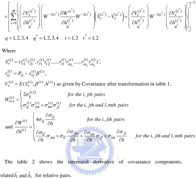
, 2 Where ( ) ( ) ( ) ( ) ( ) ( ) ( ) ( ) ( ) 1 1 1 2 1 ( ) ( ) ( ) ( ) ( ) ( ) ( ) ( , ,..., ,..., ) ', ,

( ; , ) as given by Covariance after transformation in table 1,

r r r t t t t t t t t t r r r r r r rn rn rn t t t rj rj rj t t t t r r S r r r r r r r r r P x V E S h β β = = − = ( )2 ( ) ( ) ( ) ( ) ( ) ( ) ( ) 2 , , , 4 , and t ij t r r _{t t t t} jm im il jl ij t ij t jm il jm il

for the i jth pairs W

for the i jth and l mth pairs for the i jth pairs

W h h h h σ σ σ σ σ σ σ σ σ _{σ σ} × ⎧ ⎪ = ⎨ + ⎪⎩ ∂ ∂ ∂ = ∂ ∂ _∂ + ∂ ∂ , , jl im

jl im for the i jth and l mth pairs

h h σ σ _{σ σ} ⎧ ⎪ ⎪ ⎨ ∂ ∂ ⎪ _{+ +} ⎪ _{∂ ∂} ⎩

The table 2 shows the interested derivative of covariance components,

relatedhˆ₁and hˆ₂ for relative pairs.

Table 2 The derivative of covariance components for relative pairs.

Relationship 1 V h ∂ ∂ 2 V h ∂ ∂ 1 V h ∂ ∂ 2 V h ∂ ∂ Same person 0 0 0 0 Parent-child 1/ 2h₄ 0 1/ 2 0 Full sibling 1/ 2h4 1/ 4h4 1/ 2 1/ 4 Half sibling 1/ 4h₄ 0 1/ 4 0 Monozygous twins h 4 h 4 1 1 Grandparent-grandchild 1/ 4h₄ 0 1/ 4 0 Uncle/aunt-nephew/niece 1/ 4h4 0 1/ 4 0

Based on Table 2, Heish et al. [4] express the result of the above-mentioned as follow:

(

)

* * ( ) ( ) ' ( ) ( ) ( ) 1( ) 1( ) ( ) ( ) 4 ( ) ( ) 1 1 ' ( ) ( ) ( ) 1( ) ( ) 4 _{( ) ( )} 4 ( ) ( ) 4 ₍ ˆ ˆ ( , ) ˆ ˆ ˆ ˆ ˆ ˆ t t q _q t t R t r t t t t r r t t r q q t t t r t r t t t q q t t r q Cov h h V W h W W S V h h V V h W h h h V h h − − = − − ⎡ ⎧ _{⎛ ⎞ ⎛ ⎞} ∂ ∂ ⎪ ⎢ _{⎜ ⎟ ⎜ ⎟} ≈_{⎢ ⎨} − ⎜ _∂ ⎟ ⎜ _∂ ⎟ ⎪ _{⎝ ⎠ ⎝ ⎠} ⎢ _⎩ ⎣ ⎤ ⎫ ⎛_∂ ⎞ ⎛_∂ ⎞ _⎪⎥ ⎜ ⎟ ⎜ ⎟ + _⎬⎥ ⎜_∂ ⎟ ⎜_∂ ⎟ _⎪ ⎝ ⎠ ⎝ ⎠ _⎭⎦⎥ ∂ × ∂

∑

(

)

(

)

(

)

* * * * * * * * * * * * * * * * ( ) ' ( ) 1( ) ( ) ( ) ( ) ( ) 1( ) 4 ) _{( )} 1 ' ( ) ( ) ( ) 1( ) 1( ) ( ) ( ) 4 _{( ) ( )} ˆ ˆ ˆ ˆ ˆ ˆ ˆ ˆ t R t t t t t t t r r r r r t _t r q t t t r t t t t r r t t r _{q q} V W S V S V W h h V W h W W S V h h − − = − − ⎡ ⎧ _{⎛ ⎞} ⎛ ⎞ ⎫⎤ ⎢ ⎪ _{⎜ ⎟} ⎜∂ ⎟ ⎪⎥ − − ⎢ ⎨ _{⎜ ⎟} ⎜ ⎟ ⎬⎥ ⎢ ⎪ _{⎝ ⎠} ⎜ ∂ ⎟ ⎪⎥ ⎢ ⎩ ⎝ ⎠ ⎭⎥ ⎣ ⎦ ⎧ _{⎛ ⎞ ⎛ ⎞} ⎪ _⎜∂ _{⎟ ⎜} ∂ _⎟ × _⎨ − ⎜ ⎟ ⎜ ⎟ ⎪ _⎝∂ _{⎠ ⎝} ∂ _⎠ ⎩

∑

* * * * * * * 1 1 ' ( ) ( ) ( ) 1( ) ( ) 4 _{( ) ( )} 4 * * ˆ ˆ 1, 2, 3, 4 1, 2, 3, 4 1, 2 1, 2 R t t t r t r t t t q q V V h W h h h q q t t = − − ⎡ ⎢ ⎢ ⎢ ⎣ ⎤ ⎫ ⎛_∂ ⎞ ⎛_∂ ⎞ _⎪⎥ ⎜ ⎟ ⎜ ⎟ + _{⎜ ⎟ ⎜ ⎟ ⎬⎥} ⎪ ∂ ∂ ⎥ ⎝ ⎠ ⎝ ⎠ _⎭⎦ = = = =

∑

First cousins 1/ 8h₄ 0 1/ 8 0

Double first cousins 1/ 4h4 1/16h4 1/ 4 1 /16

2.2.4 Hypothesis test

For having more statistical meaning of PHE , we utilize the confidence interval to

get more information about PHE . We hope to find a value that it means that there

exist a useful endophenotype when PHE value is larger than the value. That is, do

one-sided confidence interval.

The hypothesis is 0 1 : : H PHE a H PHE a = ⎧ ⎨ _> ⎩

Under null hypothesis and significance level ofα , we rejectH if the lower bound ₀ of one-sided confidence interval of PHE ,PHE−Z_1−α×s e PHE. .( ), is larger than a .

2.3 The whole-genome association test for quantitative outcomes

For each of the genotyped SNP markers, we are interested in testing whether

observed genotypes and quantitative phenotypes are associated. We let G_ijmdenote the observed genotype at makermfor individual j in family i .

We label two allele “A” and “a” and define a genotype score, g_ijm

0 if / 1 if / 2 if / ijm ijm ijm ijm G a a g G A a G A A ⎧ = ⎪ =_⎨ = ⎪ ₌ ⎩

First we built the model for each SNP

( _ij) _{g ij x ij}

E P = +μ β g +β x

Hereμis the population mean, β_gis the additive effect for each SNP, andβ_xis a

vector of covariate effects [19].

Chen et al. [19] extend the model with

( _ij) _{g ij x ij}

whereg is the expected genotype score and define as _ij ( | , , ) 2 ( / | , , ) ( / | , , ) ijm ijm i ijm i ijm i g E g G F P G A A G F P G A a G F θ θ θ = = = + =

whereθ is a vector of intermarker recombination fractions and F is a vector of allele frequencies for each marker. To allow for correlation between different observed

phenotypes within each family, we define the variance-covariance matrix Ω for _i family i as 2 2 2 2 2 2 , , , 2 A D C ijk ij ik A ij ik D ij ik C if j k if j k σ σ σ φ σ σ λ σ ⎧ + + = ⎪ Ω = ⎨ + Δ + ≠ ⎪⎩

Chen et al. [19] provide an approach is to first fit a simple variance-components

model to the data (with parametersμ β σ σ, _x, _A2, _R2 but without parametersβ σ_g, _D2). This model provides a vector of fitted values for each family, which they denoteE P( )_i (base), and an estimate of the variance-covariance matrix for each family, which they

denoteΩ_i(base). Using these two quantities, we define the score statistic

[

]

[

]

[

]

2 1 ( ) ( ) 1 ( ) ( ) ' ( ) ( ) ' ( ) base base i i i i i i SCORE base i i i i i i g E g y E y T g E g g E g − − ⎧ _{− ⎡Ω ⎤ ⎡ − ⎤}⎫ ⎨ _{⎣ ⎦ ⎣ ⎦}⎬ ⎩ ⎭ = ⎡ ⎤ − _⎣Ω _⎦ −

∑

∑

Whereg is a vector with expected genotype scores for each individual in the _i th

i family, calculated conditional on the available marker data, and E g( _i)is a vector with identical elements that give the unconditional expectation of each genotype score.

SCORE

T is approximately distributed as χ2with 1 df. As usual, LOD scores were defined as

2

score / 2 ln(10)

2.4 The preprocessing method for gene expression levels

We interpret the three main steps of data preprocessing.

2.4.1 Background adjustment

Because partial measured probe intensities maybe caused by non-specific

hybridization or the noise in the optical detection system, background adjustment is

essential to rid of these intensities not exactly expressed from genes. Observed probe

intensities need to be adjusted to give the accurate expression levels of specific

hybridization [20]. Some methods make use of MM probes to adjust, but some are

not.

2.4.2 Normalization

During the process of carrying out the microarray experiment involving multiple

arrays, there are many obscuring sources of variation involved, such as physical

problems with the arrays, laboratory conditions, hybridization reactions, labeling, and

scanner difference. In order to compare measurements from different arrays, implying

different tissue, some proper normalization is necessary.

2.4.3 Summarization

Due to Affymetrix platform designing multiple probes to represent a gene,

summarization is needed to combine these probe intensities to a single value. For each

gene, the background adjusted and normalized intensities are used to be summarized

into one measurement that estimates the expression level.

2.4.4 RMA ) ( : , .... , 1 : ,...., 1 ) ( : ,...., 1 gene set probe the ng representi G g gene the in pair probe the ng representi J j sample array different the ng representi I i = = =

RMA [21- 22], Robust Multi-array Analysis, is an expression measure consisting of

three particular preprocessing steps: convolution background correction, quantile

the median polish algorithm. These RMA authors proposed a procedure ignoring the

MM intensities and using only the PM intensities.

The RMA convolution background correction method is motivated by looking at

the distribution of probe intensities. The model observed PM as the sum of a

background intensity bg_ijgcaused by optical and nonspecific binding, and signal intensitys_ijg.

, 1, , , 1, , , 1, ,

ijg ijg ijg

PM =bg +s i= … I j= … J g = … G

Under the model above, the background corrected probe intensities will be given by

( _ijg)

B PM , where B PM( _ijg)≡E s( _ijg |PM_ijg). To obtain a computationally feasible

) (⋅

B we consider the closed-form transformation obtained when assuming thats_ijgis distributed exponential and bg_ijgis distributed normal, and the results obtained using

) (⋅

B work well in practice [21-22].

Next, perform the quantile normalization, which is to make the distribution of

probe intensities for each array the same [22, 23]. In order to summarize the probe

intensities, RMA introduced a log scale linear additive model. The model is:

( _ij) _{i j ij}

T PM = +e a +ε ,

where PM_ijg represents the PM intensity of array i=1,...,I and probe pair j=1,...,J, for any given probe set g. T

( )

⋅ represents the transformation that background corrects, normalizes, and logs the PM intensities, e represents the log2 _i scale expression value found on arrays i , a_j represents the log scale affinity effects for probes j , and ε represents error [22, 24]. To protect against outlier probes, they _ij

The estimate of e as the log scale measure of expression refers to as robust _i multi-array average (RMA).

2.5 The differential expression methods 2.5.1 Fold-change

Fold-change analysis is used to identify genes with expression ratios or differences

between a treatment and a control that are outside of a given cutoff or threshold.

Intensity values may be compared using ratio,log (₂ ratios , or difference. Biologist ) favors fold-change equal to 2 as the threshold of differential expression.

2.5.2 Two sample t-test

The simplest statistic method for comparing means between two groups is two

sample t-test. The variances of the two samples may be assumed to be equal or

unequal. The approach of unequal variance assumption is also called Welch’s t-test.

For any given gene g, suppose that the number of samples in sample 1 and in sample

2 are M and N respectively. Here we describe the two tests briefly.

Two sample t-test for equal variance: 2 1 1 2 1 2 0 1 2 1 1 2 2 2 2 2 1 1 1: ,...., ~ ( , ) 2 : ,..., ~ ( , ) H : : : ~ , 1 1 ( ) ( ) . 2 g gM g gN M N p M N i i i i p sample X X N sample Y Y N versus H X Y test statistic T S M N X X Y Y where S M N μ σ μ σ μ μ μ μ + − = = = ≠ − + − + − = + −

∑

∑

Two sample t-test for unequal variance (Welch’s t-test): 2 1 1 1 2 1 2 2 0 1 2 1 1 2 2 2 2 2 2 2 1 1 2 2 1: ,...., ~ ( , ) 2 : ,..., ~ ( , ) H : : : ~ ( ), ( ) 1 1 ( ) , ( ) 1 1 ( g gM g gN v X Y M N X i Y i i i X Y sample X X N sample Y Y N versus H X Y

test statistic T approximately S S M N where S X X S Y Y and M N S S M N μ σ μ σ μ μ μ μ ν = = = ≠ − + = − = − − − + =

∑

∑

2 4 4 2 2 ) . ( 1) ( 1) X Y S S M M − +N N−

After performing the test and the conclusion leads to rejectH , we consider that ₀ this gene is a differentially expressed gene.

2.5.3 SAM (Significance Analysis of Microarrays)

It was proposed by Tusher, Tibshirani and Chu (2001) [22, 25]. The method is

based on a modified version of the standard t-statistic to adjust the high variance

probably caused by a low expression level.

The “relative difference”d_g, g=1, ,pgenes:

0 g g g r d s s = +

Here r_g is a score, s_g is a standard deviation, and s is an exchangeability ₀ factor in the denominator to ensure that the variance ofd is independent of gene _g

2 1 2 2 1 2 1 2 1 2 1 2 ( ) ( ) 1 1 ( ) , 2 g g g gi g gi g i group i group g r x x x x x x s n n n n ∈ ∈ = − − + − = + × + −

∑

∑

where x_g1 and x_g2 are defined as the average levels of expression for gene g in group 1 and group 2, and x_gi is defined as the expression level for gene g and sample i. Group 1 and 2 have n and ₁ n genes, respectively. Then rank all genes by ₂ the observed relative difference d and denote the new arrangements as_g d_{( g)}. B sets

of permutations of the samples are taken to obtain the expected relative difference

* ) ( g

d by a similar way (For more details, see [22, 25-26]). A scatter plot of d_{( g)} vs.

* ) ( g

d is used and the genes apart from the * ) ( ) (g dg

d = line by a distance greater than the threshold Δ are regarded as differentially expressed genes.

2.6 Multiple testing procedures

If thousands of hypotheses are tested simultaneously, the probability of false positives

by chance increases. We use an example to understand the question: when a

two-sample t-test is performed on a gene, the probability by which the gene’s

expression level will be considered significantly different between two groups of

samples is expressed by the p-value. The p-value is the probability that a gene’s

expression levels are different between the two groups due to chance. A p-value of

0.05 signifies a 5% probability that the gene’s mean expression value in one condition

is different than the mean in the other condition by chance alone. If 10,000 genes are

Table 3 probability of calling 1 or more false positives by chance.

Number of genes

tested (N)

False positives

incidence

Probability of calling 1 or more false positives

by chance (100(1 0.95 )− N )

1 1/20 5%

2 1/10 10%

20 1 64%

100 5 99.40%

In microarray data analysis, false positives are genes that are found to be

statistically different between conditions, but are not in reality. We need to adjust

p-values derived from multiple statistical tests to correct for occurrence of false

positives.

2.6.1 Type I error rates

The null hypotheses in M tests,H₀(1),…,H M₀( ), we conduct 2 2× table to interpret the different number of tests in different conditions.

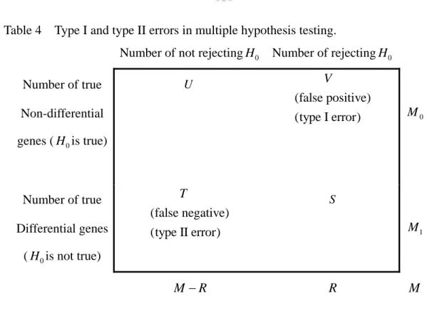
Table 4 Type I and type II errors in multiple hypothesis testing.

Number of not rejectingH₀ Number of rejectingH ₀ Number of true Non-differential genes (H is true) 0 U (false positive) (type I error) V 0 M Number of true Differential genes (H is not true) 0 (false negative) (type II error) T _S 1 M

Type I error rates is defined as a parameters,θ θ= (F_{V R,} ) , of the joint

distributionF_{V R,} of the numbers of Type I errors V and the number of rejecting hypotheses R . Such a general representation covers the following commonly-used

Type I error rates [20].

(1) Generalized family-wise error rate (gFWER), or probability of at least (k+1)

Type I errors.

( ) Pr( ).

gFWER k ≡ V >k

When k=0, the gFWER is the usual family-wise error rate (FWER), or probability

of at least one Type I error. FWER k( )≡Pr(V >0).

(2) Tail probabilities for the pro portion of false positives (TPPFP) among the

rejected hypotheses,

( ) Pr( / ), (0,1).

TPPFP q ≡ V R>q q∈

(3) False discovery rate (FDR), or expected value of the proportion of false

positives among the rejected hypotheses (Benjamini and Hochberg, 1995),

[

/

]

.

FDR≡E V R

The convention that V /R≡0 if R=0is used.

2.6.2 Adjusted p-values

Given M null hypotheses being tested H₀(1),…,H M₀( ) , the adjusted

p-valueP_0a( )m , for null hypothesisH m , is defined as the smallest Type I error ₀( ) levelα at which one would rejectH m , that is, ₀( )

[ ]

{

}

0a( ) inf 0,1 : ( ) ( ) , 1, ,

P m ≡ α∈ T m ∈C m m= … M

Where T m is the test statistic and ( ) C m is the rejection region for test( ) m .It need to have null distribution of ( )T m [22].

hypothesis is stronger. The difference between adjusted p-value and unadjusted

p-values that the unadjusted p-value,p m , for null hypothesis₀( ) H m is the smallest ₀( ) type I error rate of the single hypothesis testing procedure at which one would

rejectH m₀( ) .

2.6.3 The q-value

Storey et al. [27] define a new false discovery rate, pFDR

0

(V | 0) Pr( is true | )

pFDR E R H T C

R

= > = ∈

WhereT is the test statistic and C is the rejection region. The term ’positive’ has been

added to reflect the fact that we are conditioning on the event that positive findings

have occurred.

As a natural extension to pFDR , the q-value has the following definition [27].

Definition 1 For an observed statistic T =t, the q-value of t is defined to be

{ : }

( )

inf {

( )}

C t C

q t

pFDR C

∈

=

Definition 2 For a set of hypothesis tests conducted with independent p-values, the q-value of the observed p-value p is

( )

inf{

( )}

p

q p

pFDR

γ≥

γ

=

Where the nested set of rejection regions take the form[0, ]γ .

The q-value was discussed, which is the pFDR analogue of the p-value. Whereas it

can be inconvenient to have to fix the rejection region or the error rate beforehand, the

2.7 Datasets

The dataset we used is from the Gene Expression Omnibus (GEO) in NCBI. The

Gene Expression Omnibus (GEO) is a public repository that archives and freely

distributes microarray and other forms of high-throughput data submitted by the

scientific community. In addition to data storage, a collection of web-based interfaces

and applications are available to help users query and download the experiments and

gene expression patterns stored in GEO.

In 2007, Moffatt et al. [5] brought up this paper about asthma and offered

expression file free to download. Moffatt et al. [5] mentioned that the study subjects

were recruited from family (MRC-A) and case-control panels (MAGICS and UK-C).

The family panel included a 207 predominantly (99 %) nuclear families (MRC-A).

these were recruited through a proband with severe (step 3) childhood onset asthma

and contained 295 sib pairs, 11 half-sib pairs and 3 singletons (counting all possible

sibs). The study included siblings regardless of asthma status. Lymphoblastoid cell

lines (LCLs) were derived from peripheral blood Iymphocytes on probands and

siblings. Cells were harvested at log phase from roller cultures in the first growth after

transformation. Global gene expression in Epstein-Barr virus Iymphoblastoid cell

lines (EBVL) was measured with the Affymetrix HG-U133 Plus 2.0 chip in family

panel. The other one, in case-control panel, included 437 non-asthmatic Caucasian

UK controls (UK-C) children, 728 asthmatic children of German in the Multicentre

Asthmatic Genetics in Childhood Study (MAGICS) study with physician-diagnosed

asthma for comparison with 694 reference children recruited in the cross sectional

International Study of Asthma and Allergies in Childhood (ISAAC) study. The study

genotyped all children in the primary association study with the Illumina Sentrix

HumanHap300 BeadChip. Additional, the study typed the parents and children in the

This paper had an own database, “mRNA by SNP Browser”, that provides

graphical overviews of whole-genome association studies of datasets with very rich

phenotypic information, such as global surveys of gene expression. The software

incorporates a generic eQTL database and provides a graphic interface for browsing

association between 54,675 transcript levels and 406,912 SNPs. For each transcript,

the browser can tabulate and plot association test statistics (p-value<0.001), estimates

of effect size and allele information across the genome. The browser automatically

links results to the UCSC genome browser where users can examine each transcript in

its genomic context. In addition to browsing the results by transcript or by position,

results can be searched for information on specific SNPs. LD and tag information are

3 Materials and Methods

DNA transcribes to mRNA, mRNA translates to protein which may affect the

disease. Because mRNA is closer to DNA and gene expression value is measured in

mRNA, we use global gene expression of probe sets as endophenotypes in search for

the susceptibility genes underlying asthma. Gene expression values are preprocessed

by the robust multi-array averaging (RMA) to adjust for background noises,

normalize expression levels and summarize multiple probs. We judge which gene

expressions of probe sets are endophenotype by using the index PHE and do

hypothesis test of PHE=0 : Endophenotype and phenotype share no genes. For the

problem of multiple testing, we utilize the q-value to control for the false discovery

rate (FDR) for significance judgment. We also perform genome-wide association tests

for each gene expression of probe set.

We then derive SNPs under four conditions; they are SNPs (1) significantly

associated with gene expressions of all probes sets, (2) significantly associated with

gene expressions of probe sets with PHEs greater than zero, (3) significantly

associated with gene expressions of probe sets with PHEs significantly different from

zero at unadjusted p-values smaller than 0.05, and (4) significantly associated with

gene expressions of probe sets with PHEs significantly different from zero at q-values

smaller than 0.05.

Through systematic literature reviews (Hoffjan et al. [28], Ober et al. [29] and

Zhang et al. [30]), we identify 144 genes that have been reported to be associated with

asthma or atopy phenotypes. Among them, there are 25 genes that have been

repeatedly reported in six or more populations [29]. We further identify additional 125

genes that are related to these 25 genes. We then identify the overlap between these

analysis.

Finally, we are interests in realizing the genetic properties of gene expressions that

are identified as the endophenotypes. We use various plots to aid us observing some

phenomenon.

3.1 Datasets

In 2007, Moffatt et al. [5] brought up this paper about asthma. The subjects of this

study can be divided into two master parts: the case-control panel and the family

panel. We are interested in the family panel. There are 404 children from the family

panel. The family panel included 207 predominantly (99 %) nuclear families. These

were recruited through a proband with severe childhood onset asthma. The study

included siblings regardless of asthma status. Global gene expression in Epstein-Barr

virus Iymphoblastoid cell lines (EBVL) was measured with the Affymetrix HG-U133

Plus 2.0 chip in the family panel. The study genotyped 830 offspring and parents with

the Illumina Sentrix HumanHap-I BeadChip and 378 offspring with the Illumina

Sentrix HumanHap300 BeadChip in family panel.

We downloaded the files of Gene expression levels in 404 children from the family

panel. This dataset is available at 8http://www.ncbi.nlm.nih.gov/ego/, the GEO

accession: GSE8052 [6].

3.2 Statistical method of endophenotype

We use global gene expressions of probe sets as endophenotypes. Epstein-Barr

virus Iymphoblastoid cell lines (EBVL) were derived from participants and global

gene expression was measured with Affymetrix HG-U133 Plus 2.0 chip. One of the

indices determining the gene expression of probe set an endophenotype is the

proportion of heritability explained (PHE) by the endophenotype [2].

2 2 2 2 2 2 2 , , , , (0, ) (0,[ ]) cov( , ) 2 , ij H H ij H ij ij ij ij R ij A D C ij ik ij ik A ij ik D ij ik C P E Z G Normal G Normal G G j k α γ τ ε ε σ σ σ σ φ σ σ λ σ = + + + + + + = + Δ + ≠ ∼ ∼

WhereP is the observed phenotype in the jth member of the ith family,_ij E is his/her _ij

corresponding specified endophenotype, Z is his/her other covariates._ij ε_ij is the

residual error term representing the effect of non-family factors.G is the random _ij

effect for the underlying genetic structure. The componentsσ σ2_A, _D2 and σ_C2represent the variance arising from polygenic additive effects, polygenic dominance effects and

shared environmental effects, respectively.

The (broad sense) heritability ofP , conditional on_ij E is _ij

2 2 2 2 2 2 A D A D C R h σ σ σ σ σ σ + = + + +

Then we calculate PHEs of all probe sets.

1 NE h PHE h = −

Where the term h is the heritability calculated from the variance component analysis

with disease status as response variable and covariates including the endophenotype

and other covariates. The term h_NE is the heritability calculated from the variance component analysis with disease status as response variable and covariates without

endophenotype [2]. The greater of the PHE value, the more likely he intermediate

variable an endophenotype. Hsieh et al. [4] utilize the delta method to evaluate the

variance of PHE. For having more statistical meanings of PHE, We do hypothesis test

The hypothesis is 0 1 : 0 : 0 H PHE H PHE = ⎧ ⎨ _> ⎩

UnderH₀:PHE= , we suppose the phenotype and endophenotype share no genes 0 and significance level ofα =0.05. We rejectH if the lower bound of one-sided ₀

confidence interval of PHE ,PHE−Z_1−α×s e PHE. .( ), is larger than 0 and plot the confidence of interval of PHEs over all chromosomes.

If multiple hypotheses are tested simultaneously, the probability of false positives

by chance increases. We utilize the q-value which is a natural pFDR analogue of the

p-value to correct for occurrence of false positives. These q-values were calculated by

applying the QVALUE (8http://faculty.washington.edu/~jstorey/qvalue/) package.

Wherehandh_NEwere obtained from the results by performing variance component analysis using the SOLAR computer package [14], so PHE is estimated. The estimator ofs e PHE. .( )used delta method [4].

Then we classify PHEs into four conditions, there are total PHEs, PHEs higher than

zero, significant PHEs with unadjusted p-value smaller than the significant level of

5%, and significant PHEs with q-value smaller than the significant level of 5%.

3.3 The preprocessing and differential method

All analyses of expression value used quantile normalization, after performing

robust multi-array averaging (RMA), to remove non-biological variation, enforce

normality, deal with outlier and summary the intensity values [21-22, 24].

We want to know if a disease may be caused by large expression of particular genes

significance analysis of Microarrays (SAM) [22, 25-26]. The term q-value in SAM

output smaller than 0.05, it represents these probe sets may be different between

diseased and normal subset.

3.4 Genome-wide association tests for gene expressions

A database, “mRNA by SNP Browser”, that provides the results of Genome-wide

association test for each gene expression of probe set [31]. Association analysis was

applied with Merlin (FASTASSOC option), after probabilistically inferring missing

genotypes. This database is downloaded at

8

http://www.sph.umich.edu/csg/liang/asthma/.

We find significant SNPs from results of associate test between expression value of

each probe set and all SNPs genotypes with LOD score≥ 6 (about equivalent to the false discovery rate (FDR) = 0.056) [6]. We define these significant SNPs as

“eSNPs”.

3.5 Asthma genes and overlap rate

Asthma is a disease of chronic airway inflammation that affects nearly 155 million

individuals worldwide. Like other atopic diseases, asthma is a complex disorder

caused by interactions between multiple genes of small to modest effect and equally

important environmental factors. Asthma has an important genetic component but no

clear pattern of inheritance and heritability estimates of asthma vary between 36-79%.

To this day, there are over 100 genes that have been reported to be associated with

asthma or related phenotypes. We look for three review papers: (1) “Association

studies for asthma and atopic diseases: a comprehensive review of the literature” [28],

there are 64 genes in 251 papers about asthma or atopy from 1982 to 2002, (2)