國 立 交 通 大 學
應用化學系分子科學碩士班
碩 士 論 文
利用法蘭克-康登擬合綠色螢光蛋白質發色團的
吸收與螢光光譜
Franck-Condon Simulation of Absorption and
Fluorescence Spectra for GFP Chromophore
研 究 生: 黃琮偉 (Tsung-Wei Huang)
指導教授: 朱超原 (Chao-Yuan Zhu)
i
利用法蘭克-康登擬合綠色螢光蛋白質發色團的
吸收與螢光光譜
研究生
:
黃琮偉
指導教授: 朱超原
國立交通大學應用化學系分子科學碩士班
摘要
綠色螢光蛋白質的發色團是經過分子內的一些反應而形成,由第 65 號的絲胺 酸(serine-65)、第 66 號的酪胺酸(tyrosin-66)和第 67 號的甘胺酸(glycine-67)組成主 要的結構,而紅色螢光蛋白質的發色團則是由第 66 號的谷氨醯胺(glutamine-66)、 第 67 號的酪胺酸(tyrosin-67)和第 68 號的甘胺酸(glycine-68)所組成。綠色以及紅 色螢光蛋白質的發色團同時具有 4-hydroxybenzylideneimidazolinone 的部分,但 imidazolinone ring 所連接的官能基則不同。將兩者發色團的吸收性質互相比較, 若所連接的官能基是Π 共軛系統,將會造成明顯的紅位移。 在本研究工作裡,我們主要使用法蘭克-康登擬合(Franck-Condon simulation) 綠色和紅色螢光蛋白質之發色團的吸收以及螢光光譜,而法蘭克-康登擬合的過 程包含了均勻與非均勻加寬和簡諧與非簡諧的討論。在基態的計算方面,則使用 了三種不同交換−相關效應的密度泛函(B3LYP, B3LYP-35, and BHandHLYP)和 Hartree-Fock 方法,結合使用極化連續模型來計算溶劑效應。而在激發態的計算 方面,則必須基於使用相同層級的 ab initio 方法,例如含時密度泛函理論(TD-DFT) 對應密度泛函理論(DFT)、單電子激發組態交互作用(CIS)則對應 Hartree-Fock 方ii
法。
本研究成果成功的論述了 HBDI 的吸收和螢光光譜,不論是在譜峰的位置,抑 或是光譜的寬度,與實驗光譜相比都具有很好的一致性。
iii
Franck-Condon Simulation of Absorption and Fluorescence
Spectra for GFP Chromophore
Student: Tsung-Wei Huang Advisor: Dr. Chao-Yuan Zhu
Department of Applied Chemistry and Institute of Molecular
Science
National Chiao Tung University
ABSTRACT
The GFP chromophore is formed by the intramolecular reaction from tripeptide serine-65 (Ser65), tyrosin-66 (Tyr66), and glycine-67 (Gly67) in the native protein for the primary structure while the chromophore in DsRed is also formed from the three amino acids which are glutamine-66 (Gln66), tyrosin-67 (Tyr67), and glycine-68 (Gly68) for the primary structure. Both the GFP and DsRed chromophores share the same 4-hydroxybenzylideneimidazolinone core, but the linkages at the imidazolinone ring are different. The extension of the conjugated Π-system in the chromophore may cause the significant red shift of the DsRed absorption properties compared to those of GFP.
In the present work, we demonstrate the absorption and fluorescence spectra of the GFP and DsRed chromophore in Franck-Condon simulation with including homogenous broadening, inhomogenous broadening, harmonic, and anharmonic
iv
discussions. Three different exchange-correlation functionals (B3LYP, B3LYP-35, and BHandHLYP) of density functional theory (DFT) and Hartree-Fock (HF) method with and without the polarizable continuum model (PCM) were used for the ground state. At the same level of ab initio methods for the excited states, time-dependent density functional theory (TD-DFT) verse DFT and configuration interaction singles (CIS) verse HF, respectively.
The results presented in this study demonstrate that peak position and spectral widths of both absorption and fluorescence spectra for HBDI agree with experimental observations.
v
誌謝
兩年,在交大完成了碩士學位,一個人生旅途中的里程碑。 研究的過程雖然艱辛但成功的果實總是甜美。首先,萬分感謝朱超原老師以及 林聖賢老師,給予我在研究上的指點迷津抑或是解決我在課業上的疑惑。感謝實 驗室的琇雅學姊、哲源學長、孔哥令鈞、俊吉、李清旭學長、楊林學姊、李軍學 長、宋迪學姊、雷依波學長、羅格非、易軍學姊、牛英利學長、莫燕學姊、孫廣 旭、閻林胤、 Teranishi、Yamaki、美婷,給予我各方面的支持,讓這原本枯燥乏 味的研究生活,增添了些許的色彩。感謝我的室友們-在睡夢中不忘研究的鎮廷、 愛打球的虎牙哥富全、不離不棄是我兄弟的純情小綿羊哲豪,總在那夜深人靜時, 想起那些一起度過的夜晚。感謝籃球社的籃球甜心璟妤社長、一起擊退硬課的偲 丞、新任室友並肩作戰抵抗宅宅的岡岡、無私分享真的很黑的彥勳、很久沒來打 球的小雞鈺芳、沒打過球卻很愛胸毛的小阿芳郁芳、以及一起打過球或是給予我 幫助的各位學長同學們。 最後,感謝我的家人們,將這份榮耀與你們一起分享。 琮偉 謹誌 100 年 7 月 新竹交大vi
Table of Contents
摘要... i
ABSTRACT ... iii
誌謝... v
List of Tables ... viii
List of Figures ... xi
I. Chapter 1 Introduction ... 1
II. Chapter 2 Theory ... 7
2.1 Density Functional Theory (DFT) ... 7
2.2 Time-Dependent Density Functional Theory (TD-DFT) ... 10
2.3 The Brief Polarizable Continuum Model (PCM) Method... 11
2.4 Principles for Absorption and Fluorescence Spectra ... 12
III. Chapter 3 Computational Methods ... 19
IV. Chapter 4 Results and Discussion ... 21
4.1 HBDI ... 21
4.1.1 Geometries of HBDI for CS Symmetry ... 21
4.1.2 Vibrational Frequencies of HBDI for CS Symmetry ... 23
4.1.3 Absorption Spectra of HBDI for CS Symmetry ... 27
4.1.4 Geometries of HBDI for C1 Symmetry ... 29
4.1.5 Vibrational Frequencies of HBDI for C1 Symmetry ... 35
4.1.6 Absorption and Fluorescence Spectra of HBDI for C1 Symmetry ... 44
4.1.7 Anharmonic Franck-Condon Simulation of Absorption and Fluorescence Spectra for C1 Symmetry ... 72
4.1.8 Excitation Energy and Oscillator Strength of HBDI for C1 Symmetry 77 4.2 HBI ... 80
vii
4.2.2 Vibrational Frequencies of HBI for C1 Symmetry ... 82
4.2.3 Absorption Spectra of HBI for C1 Symmetry ... 88
4.2.4 Excitation Energy and Oscillator Strength of HBI for C1 Symmetry .. 91
4.3 wt-GFP ... 94
4.3.1 Geometries of wt-GFP for C1 Symmetry ... 94
4.3.2 Absorption Spectra of wt-GFP for C1 Symmetry... 95
4.4 HBMPI ... 96
4.4.1 Geometries of HBMPI for C1 Symmetry ... 96
4.4.2 Vibrational Frequencies of HBMPI for C1 Symmetry ... 97
4.4.3 Absorption Spectra of HBMPI for C1 Symmetry ... 98
V. Chapter 5 Conclusions ...100
viii
List of Tables
Table 1 Unscaled calculated vibrational frequencies of S0 (j, cm
-1
) and S1 (j, cm
-1
) states with Cs symmetry using B3LYP/TD-B3LYP method. The corresponding Huang-Rhys factors (S HF, dimensionless) are also shown. ... 25 Table 2 Unscaled calculated vibrational frequencies of S0 (j, cm
-1
) and S1 states
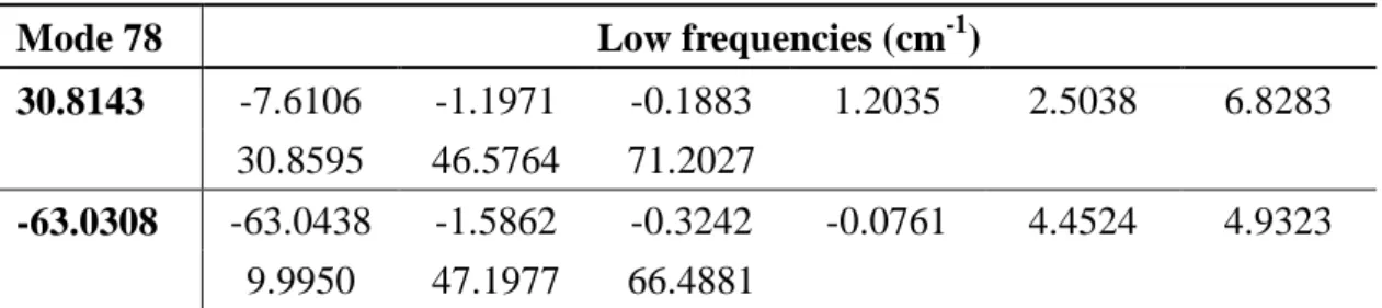
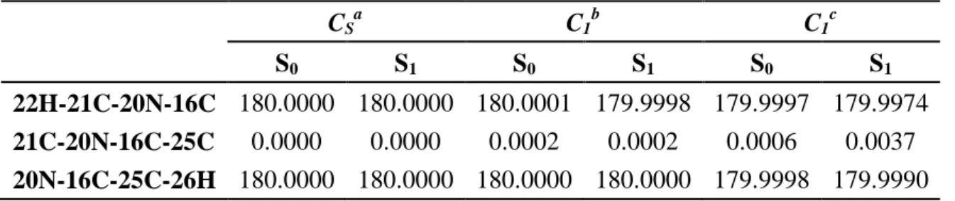
(j, cm-1) with Cs symmetry using HF/CIS method. The corresponding Huang-Rhys factors (S HF, dimensionless) are also shown. ... 26 Table 3 Important dihedral angles (in degree) of ground and first singlet excited states for CS and C1 symmetry. ... 31 Table 4 X-ray crystal structure from Ref. [46]. ... 34 Table 5 Calculated low frequencies of translation and rotation modes for mode 78 by TD-B3LYP method. ... 37 Table 6 Unscaled calculated vibrational frequencies of S0 (j, cm
-1
) and S1 (j, cm
-1
) with C1 symmetry using B3LYP/TD-B3LYP method. The corresponding Huang-Rhys factors (S HF, dimensionless) and the 3rd derivative of S0
potential energy surface (Kj3, Hartree*amu
-3/2
*Bohr-3) are also shown. ... 39 Table 7 Unscaled calculated vibrational frequencies of S0 (j, cm
-1
) and S1 (j, cm
-1
) states with C1 symmetry using B3LYP/TD-B3LYP method. The corresponding Huang-Rhys factors ( S HF , dimensionless) and the 3rd derivative of S0 potential energy surface (Kj3, Hartree*amu
-3/2
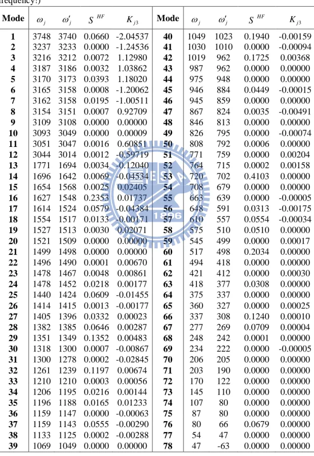
*Bohr-3) are also shown. (One imaginary frequency!) ... 40 Table 8 Unscaled calculated vibrational frequencies of S0 (j, cm
-1
) and S1 (j, cm
-1
) states with C1 symmetry using B3LYP-35/TD-B3LYP-35 method. The corresponding Huang-Rhys factors ( S HF , dimensionless) and the 3rd derivative of S0 potential energy surface (Kj3, Hartree*amu
-3/2
*Bohr-3) are also shown. ... 41 Table 9 Unscaled calculated vibrational frequencies of S0 (j, cm
-1
) and S1 (j, cm
-1
) states with C1 symmetry using BHandHLYP/TD-BHandHLYP method. The corresponding Huang-Rhys factors ( S HF , dimensionless) and the 3rd derivative of S0 potential energy surface (Kj3, Hartree*amu
-3/2
*Bohr-3) are also shown. ... 42 Table 10 Unscaled calculated vibrational frequencies of the S0 (j, cm
-1
ix
cm-1) states with C1 symmetry using HF/CIS method. The corresponding Huang-Rhys factors (S HF, dimensionless) and the 3rd derivative of S0
potential energy surface (Kj3, Hartree*amu-3/2*Bohr-3) are also shown. ... 43 Table 11 Calculated vibrational frequencies (cm-1) for ground state and the corresponding Huang-Rhys factors (dimensionless). The frequencies multiplied by scaling factor (0.9614) are provided in the brackets. ... 51 Table 12 Comparison of corresponding vibrational frequencies (cm-1) modes with its Huang-Rhys factors (SHR, dimensionless) between one and no imaginary frequency for S1. ... 65
Table 13 Vertical and adiabatic excitation energies (eV) for TD-B3LYP, TD-B3LYP-35, TD-BHandHLYP , and CIS calculations. ... 77 Table 14 Vertical and adiabatic excitation energies (eV) for TD- B3LYP with PCM (Acetonitrile, Methanol, and THF) calculations. ... 78 Table 15 Vertical excitation energies (eV) for previous studies, TD-DFTa, CIS, and ZINDO methods. Oscillator strengths are provided in the brackets. ... 79 Table 16 Vibrational frequencies (cm-1) in the region 1000−3600 cm-1 for experiment and calculations. The sacling factors are 0.9614 for B3LYP/6-31+G(d), 0.94 for B3LYP-35/6-31+G(d), 0.92 for BHandHLYP/6-31+G(d), and 0.8970 for HF/6-31+G(d), respectively. ... 83 Table 17 Unscaled calculated vibrational frequencies of S0 (j, cm
-1
) and S1 (j,
cm-1) with C1 symmetry using B3LYP/TD-B3LYP method. The corresponding Huang-Rhys factors ( S HF , dimensionless) and the 3rd derivative of S0 potential energy surface (Kj3, Hartree*amu
-3/2
*Bohr-3) are also shown. ... 84 Table 18 Unscaled calculated vibrational frequencies of S0 (j, cm
-1
) and S1 (j,
cm-1) with C1 symmetry using B3LYP-35/TD-B3LYP-35 method. The corresponding Huang-Rhys factors ( S HF , dimensionless) and the 3rd derivative of S0 potential energy surface (Kj3, Hartree*amu
-3/2
*Bohr-3) are also shown. ... 85 Table 19 Unscaled calculated vibrational frequencies of S0 (j, cm
-1
) and S1 (j,
cm-1) with C1 symmetry using BHandHLYP/TD-BHandHLYP method. The corresponding Huang-Rhys factors ( S HF , dimensionless) and the 3rd derivative of S0 potential energy surface (Kj3, Hartree*amu
-3/2
*Bohr-3) are also shown. ... 86
x
Table 20 Unscaled calculated vibrational frequencies of S0 (j, cm
-1
) and S1 (j,
cm-1) with C1 symmetry using HF/CIS method. The corresponding Huang-Rhys factors (S HF, dimensionless) and the 3rd derivative of S0
potential energy surface (Kj3, Hartree*amu-3/2*Bohr-3) are also shown. ... 87 Table 21 Vertical and adiabatic excitation energies (eV) for TD-B3LYP, TD-B3LYP-35, TD-BHandHLYP , and CIS calculations. ... 92 Table 22 Vertical and adiabatic excitation energies (eV) for TD- B3LYP with PCM (Acetonitrile, 1,2-ethanediol, and water) calculations. ... 92 Table 23 Vertical excitation energies (eV) for previous studies, TD-DFTa, CIS, and ZINDO methods. Oscillator strengths are provided in the brackets. ... 93 Table 24 Unscaled calculated vibrational frequencies of the S0 (j, cm
-1
) and S1 (j,
cm-1) for C1 symmetry using B3LYP/TD-B3LYP method. The corresponding Huang-Rhys factors (S HF, dimensionless) and the 3rd derivative of S0
xi
List of Figures
Fig. 1 The bioluminescent organ is located along the umbrella-like edge [1]. ... 1 Fig. 2 The three-dimensional structure of the GFP which was first solved in 1996 independently by Ormö et al. (The figure were obtained from the Protein Data Bank (PDB) access code 1EMA.) ... 3 Fig. 3 The biosynthetic mechanism for the formation of the GFP chromophore. ... 4 Fig. 4 Oxidation of Tyr66 leads into forming two fluorescent states – the neutral (protonated) and anionic (deprotonated) species. ... 4 Fig. 5 Optimized geometries in gas phase of the Cs symmetry S0 and S1 states for
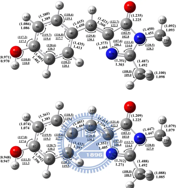
HBDI. (Top) from B3LYP/6-31+G(d) and TD-B3LYP/6-31+G(d) calculations, (Bottom) from HF/6-31+G(d) and CIS/6-31+G(d) calculations. The bond lengths (bold, in angstrom) and angles (underline, in degree) of S1
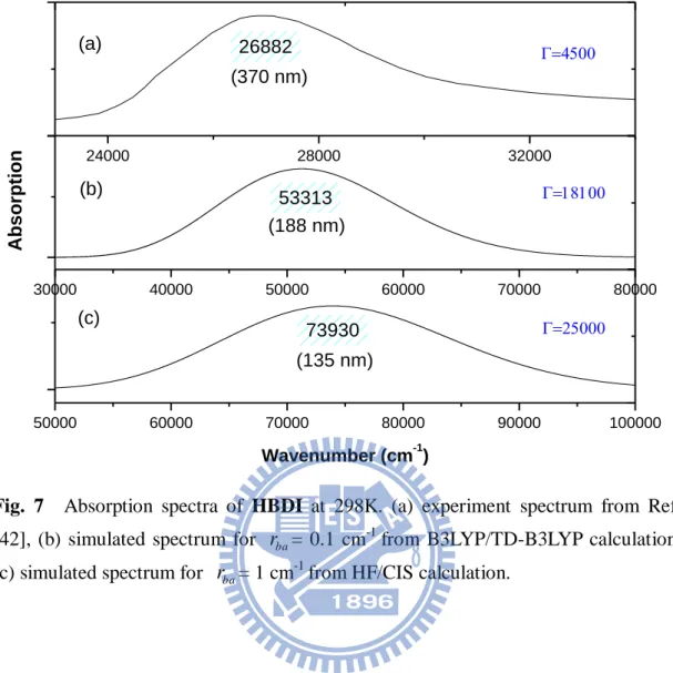
are provided in the brackets. ... 22 Fig. 6 Infrared spectra of HBDI. (a) experimental spectrum from Ref. [23], (b) B3LYP/6-31+G(d) calculation for CS symmetry of the ground state, (c) HF/6-31+G(d) calculation for CS symmetry of the ground state. The frequencies multiplied by scaling factor 0.9614 for B3LYP/6-31+G(d) method and 0.8970 for HF/6-31+G(d) method, respectively. ... 23 Fig. 7 Absorption spectra of HBDI at 298K. (a) experiment spectrum from Ref. [42],
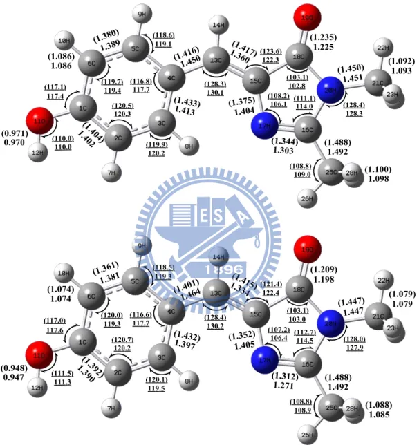
(b) simulated spectrum for rba = 0.1 cm-1 from B3LYP/TD-B3LYP calculation, (c) simulated spectrum for r = 1 cmba -1 from HF/CIS calculation. ... 28 Fig. 8 Optimized geometries of the S0 and S1 states for HBDI. (Top)
B3LYP/6-31+G(d) and TD-B3LYP/6-31+G(d) calculation (Bottom) HF/6-31+G(d) and CIS/6-31+G(d) calculation. The bond lengths (bold, in angstrom) and angles (underline, in degree) of S1 are provided in the brackets.
... 30 Fig. 9 B3LYP/6-31+G(d) and TD-B3LYP/6-31+G(d) optimized geometries of the S0 and S1 states for HBDI. (Top) acetonitrile solvent, (Middle) methanol
solvent, and (Bottom) THF solvent for PCM calculations. The bond lengths (bold, in angstrom) and angles (underline, in degree) of S1 are provided in the
brackets. ... 32 Fig. 10 Infrared spectra of HBDI. (a) experimental spectrum from Ref. [23], (b)
xii
B3LYP/6-31+G(d) method for C1 symmetry of the ground state, (c) B3LYP-35/6-31+G(d) method for C1 symmetry of the ground state, (d) BHandHLYP/6-31+G(d) method for C1 symmetry of the ground state, (e) HF/6-31+G(d) method for C1 symmetry of the ground state. The frequencies multiplied by scaling factor 0.9614 for B3LYP/6-31+G(d) method, 0.94 for B3LYP-35/6-31+G(d) method, 0.92 for B3LYP/6-31+G(d) method, and 0.8970 for HF/6-31+G(d) method, respectively. ... 36 Fig. 11 Absorption spectra of HBDI at 298K. (a) Experimental spectrum from Ref. [42] , (b) simulated spectrum for r = 10 cmba -1 and D = 800 cmba -1 from B3LYP/TD-B3LYP with PCM (Methanol) method, (c) simulated spectrum for r = 10 cmba -1 and D = 800 cmba -1 from B3LYP/TD-B3LYP calculation, (d) simulated spectrum for r = 10 cmba -1 and D = 800 cmba -1 from HF/CIS calculation. ... 45 Fig. 12 Simulated absorption spectra of HBDI in various solvents at 298K. (a)
acetonitrile, (b) methanol, (c) THF. All the spectra were simulated for r = ba
10 cm-1 and D = 800 cmba -1 ... 46 Fig. 13 Fluorescence spectra of HBDI at 298K (a) Experimental spectrum from Ref. [42], (b) simulated spectrum for r = 10 cmba -1 and D = 500 cmba -1 from B3LYP/TD-B3LYP with PCM (Methanol) calculation, (c) simulated spectrum for r = 10 cmba -1 and D = 400 cmba -1 from B3LYP/TD-B3LYP calculation, (d) simulated spectrum for r = 10 cmba -1 and D = 700 cmba -1
from HF/CIS calculation. ... 47 Fig. 14 Fluorescence spectra at 77K (a) Experimental spectrum from Ref. [16], (b) simulated spectrum for rba = 10 cm-1 and Dba = 450 cm-1 from B3LYP/TD-B3LYP with PCM (THF) calculation, (c) simulated spectrum for
ba
r = 10 cm-1 and D = 400 cmba -1 from B3LYP/TD-B3LYP calculation, (d) simulated spectrum for r = 10 cmba -1 and D = 300 cmba -1 from HF/CIS calculation. ... 49 Fig. 15 Simulated absorption spectrum (Top, at 298K) and fluorescence spectrum (Bottom, at 77K) of HBDI using B3LYP/TD-B3LYP calculation. The stick spectrum represents the Frank-Condon factors and the important band lines are assigned for comparison. All the spectra were simulated for r = 1 cmba -1
and D = 1 cmba -1. ... 50 Fig. 16 Mode 16 of gas phase in B3LYP/TD-B3LYP calculation. The purple and
xiii
orange arrows represent displacement vectors and dipole derivative vector, respectively... 51 Fig. 17 Mode 29 of gas phase in B3LYP/TD-B3LYP calculation. The purple arrows represent the displacement vectors and the orange arrow represents dipole derivative vector. ... 52 Fig. 18 Mode 32 of gas phase in B3LYP/TD-B3LYP calculation. The purple arrows represent the displacement vectors and the orange arrow represents dipole derivative vector. ... 52 Fig. 19 Mode 40 of gas phase in B3LYP/TD-B3LYP calculation. The purple arrows represent the displacement vectors and the orange arrow represents dipole derivative vector. ... 53 Fig. 20 Mode 42 of gas phase in B3LYP/TD-B3LYP calculation. The purple and orange arrows represent displacement vectors and dipole derivative vector, respectively... 53 Fig. 21 Mode 53 of gas phase in B3LYP/TD-B3LYP calculation. The purple and orange arrows represent displacement vectors and dipole derivative vector, respectively... 54 Fig. 22 Mode 60 of gas phase in B3LYP/TD-B3LYP calculation. The purple and orange arrows represent displacement vectors and dipole derivative vector, respectively... 54 Fig. 23 Mode 66 of gas phase in B3LYP/TD-B3LYP calculation. The purple and orange arrows represent displacement vectors and dipole derivative vector, respectively... 55 Fig. 24 Mode 76 of gas phase in B3LYP/TD-B3LYP calculation. The purple and orange arrows represent displacement vectors and dipole derivative vector, respectively... 55 Fig. 25 Mode 16 in B3LYP/TD-B3LYP with PCM (methanol) calculation. The purple and orange arrows represent displacement vectors and dipole derivative vector, respectively. ... 56 Fig. 26 Mode 29 in B3LYP/TD-B3LYP with PCM (methanol) calculation. The purple and orange arrows represent displacement vectors and dipole derivative vector, respectively. ... 56 Fig. 27 Mode 32 in B3LYP/TD-B3LYP with PCM (methanol) calculation. The purple and orange arrows represent displacement vectors and dipole
xiv
derivative vector, respectively. ... 57 Fig. 28 Mode 40 in B3LYP/TD-B3LYP with PCM (methanol) calculation. The purple and orange arrows represent displacement vectors and dipole derivative vector, respectively. ... 57 Fig. 29 Mode 42 in B3LYP/TD-B3LYP with PCM (methanol) calculation. The purple and orange arrows represent displacement vectors and dipole derivative vector, respectively. ... 58 Fig. 30 Mode 53 in B3LYP/TD-B3LYP with PCM (methanol) calculation. The purple and orange arrows represent displacement vectors and dipole derivative vector, respectively. ... 58 Fig. 31 Mode 60 in B3LYP/TD-B3LYP with PCM (methanol) calculation. The purple and orange arrows represent displacement vectors and dipole derivative vector, respectively. ... 59 Fig. 32 Mode 66 in B3LYP/TD-B3LYP with PCM (methanol) calculation. The purple and orange arrows represent displacement vectors and dipole derivative vector, respectively. ... 59 Fig. 33 Mode 75 in B3LYP/TD-B3LYP with PCM (methanol) calculation. The purple and orange arrows represent displacement vectors and dipole derivative vector, respectively. ... 60 Fig. 34 Mode 16 in B3LYP/TD-B3LYP with PCM (THF) calculation. The purple and orange arrows represent displacement vectors and dipole derivative vector, respectively. ... 60 Fig. 35 Mode 29 in B3LYP/TD-B3LYP with PCM (THF) calculation. The purple and orange arrows represent displacement vectors and dipole derivative vector, respectively. ... 61 Fig. 36 Mode 32 in B3LYP/TD-B3LYP with PCM (THF) calculation. The purple and orange arrows represent displacement vectors and dipole derivative vector, respectively. ... 61 Fig. 37 Mode 40 in B3LYP/TD-B3LYP with PCM (THF) calculation. The purple and orange arrows represent displacement vectors and dipole derivative vector, respectively. ... 62 Fig. 38 Mode 42 in B3LYP/TD-B3LYP with PCM (THF) calculation. The purple and orange arrows represent displacement vectors and dipole derivative vector, respectively. ... 62
xv
Fig. 39 Mode 53 in B3LYP/TD-B3LYP with PCM (THF) calculation. The purple and orange arrows represent displacement vectors and dipole derivative vector, respectively. ... 63 Fig. 40 Mode 60 in B3LYP/TD-B3LYP with PCM (THF) calculation. The purple and orange arrows represent displacement vectors and dipole derivative vector, respectively. ... 63 Fig. 41 Mode 66 in B3LYP/TD-B3LYP with PCM (THF) calculation. The purple and orange arrows represent displacement vectors and dipole derivative vector, respectively. ... 64 Fig. 42 Mode 75 in B3LYP/TD-B3LYP with PCM (THF) calculation. The purple and orange arrows represent displacement vectors and dipole derivative vector, respectively. ... 64 Fig. 43 Simulated absorption spectra of HBDI at 2K. (a) for r = 5 cmba -1 from B3LYP/TD-B3LYP calculation with no imaginary frequency, (b) for r = 10 ba
cm-1 from B3LYP/TD-B3LYP calculation with no imaginary frequency. .. 66 Fig. 44 Simulated absorption spectra of HBDI at 2K without scaling factor. (a) for
ba
r = 5 cm-1 from B3LYP/TD-B3LYP calculation, (b) for rba = 10 cm-1 from B3LYP/TD-B3LYP calculation. ... 67 Fig. 45 Simulated absorption spectra of HBDI at 2K without scaling factor. (a) for
ba
r = 5 cm-1 from B3LYP-35/TD-B3LYP-35 calculation, (b) for r = 10 cmba -1
from B3LYP-35/TD-B3LYP-35 calculation. ... 68 Fig. 46 Simulated absorption spectra of HBDI at 2K without scaling factor. (a) for
ba
r = 5 cm-1 from BHandHLYP/TD-BHandHLYP calculation, (b) for r = 10 ba
cm-1 from BHandHLYP/TD-BHandHLYP calculation. ... 69 Fig. 47 Simulated absorption spectra of HBDI at 2K without scaling factor. (a) for
ba
r = 5 cm-1 from HF/CIS calculation, (b) for r = 10 cmba -1 from HF/CIS calculation. ... 70 Fig. 48 Simulated absorption spectra of HBDI at 2K. (a) for r = 5 cmba -1,and D = ba
700 cm-1 from B3LYP-35/TD-B3LYP-35 calculation with scaling factor 0.94,
(b) for rba = 10 cm-1, and Dba = 500 cm-1 from
BHandHLYP/TD-BHandHLYP calculation with scaling factor 0.92. ... 71 Fig. 49 Absorption spectra of HBDI at 298K. (a) Experimental spectrum from Ref. [42], (b) anharmonic simulated spectrum for r = 10 cmba -1, D = 800 cmba -1, and the first-order anharmonic effect = 0.3 from B3LYP/TD-B3LYP with
xvi
PCM (Methanol) calculation, (c) anharmonic simulated spectrum for r = ba
10 cm-1, D = 800 cmba -1, andthe first-order anharmonic effect = 0.3 from B3LYP/TD-B3LYP calculation, ... 73 Fig. 50 Anharmonic simulated absorption spectra of HBDI in various solvents at 298K. (a) acetonitrile, (b) methanol, (c) THF. All the spectra were simulated for r = 10 cmba -1, D = 800 cmba -1, and the first-order anharmonic effect = 0.3 except THF (0.25). ... 74 Fig. 51 Fluorescence spectra at 298K (a) Experimental spectrum from Ref. [42], (b) simulated spectrum for r = 10 cmba -1, D = 500 cmba -1,and the first-order anharmonic effect = 0.3 from B3LYP/TD-B3LYP with PCM (Methanol) calculation, (c) simulated spectrum for r = 10 cmba -1, D = 400 cmba -1,and the first-order anharmonic effect = 0.3from B3LYP/TD-B3LYP calculation. ... 75 Fig. 52 Fluorescence spectra at 77K (a) Experimental spectrum from Ref. [16], (b) simulated spectrum for r = 10 cmba -1,D = 450 cmba -1,and the first-order anharmonic effect = 0.3 from B3LYP/TD-B3LYP with PCM (THF) calculation, (c) simulated spectrum for r = 10 cmba -1, D = 400 cmba -1,and the first-order anharmonic effect = 0.3from B3LYP/TD-B3LYP calculation. ... 76 Fig. 53 B3LYP/6-31+G(d) and TD-B3LYP/6-31+G(d) optimized geometries of the S0 and S1 states for the anionic HBI. (Top) gas phase, (Middle)
1,2-ethanediol solvent for PCM calculation, and (Bottom) water solvent for PCM calculation. The bond lengths (bold, in angstrom) and angles (underline, in degree) of S1 are provided in the brackets. ... 81
Fig. 54 Absorption spectra of the anionic HBI at 77K. (a) Experiment spectrum from Ref. [13], (b) simulated spectrum for rba = 10 cm-1 from B3LYP/TD-B3LYP calculation, (c) simulated spectrum for r = 5 cmba -1 from B3LYP-35/TD-B3LYP-35 calculation, (d) simulated spectrum for r = 5 ba
cm-1 from BHandHLYP/TD-BHandHLYP calculation, (E) simulated spectrum for r = 5 cmba -1 from HF/CIS calculation. ... 89 Fig. 55 Absorption spectra of the anionic HBI at 77K for PCM method. (a) Experiment spectrum from Ref. [13], (b) simulated spectrum for r = 10 ba
cm-1 from B3LYP/TD-B3LYP with PCM (acetonitrile) calculation, (c) simulated spectrum for r = 10 cmba -1 from B3LYP/TD-B3LYP with PCM
xvii
(1,2-ethanediol) calculation, (d) simulated spectrum for r = 10 cmba -1 from B3LYP/TD-B3LYP with PCM (water) calculation. ... 90 Fig. 56 Simulated absorption spectra of the anionic HBI at 77K. (a) for r = 5 cmba -1,
and D = 15 cmba -1 from B3LYP/TD-B3LYP calculation, (b) for r = 5 cmba -1, and D = 30 cmba -1 from B3LYP/TD-B3LYP calculation, (c) for r = 5 cmba -1, and D = 100 cmba -1 from B3LYP/TD-B3LYP calculation, (d) for r = 5 cmba -1, and D = 500 cmba -1 from B3LYP/TD-B3LYP calculation. ... 91 Fig. 57 B3LYP/6-31+G(d) and TD-B3LYP/6-31+G(d) optimized geometries of the S0 and S1 states for the anionic form of the wt-GFP in gas phase. ... 94
Fig. 58 Absorption spectra of the anionic form of the wt-GFP at 77K. (a) Experiment spectrum from Ref. [13], (b) simulated spectrum for r = 10 ba
cm-1 from B3LYP/TD-B3LYP calculation. ... 95 Fig. 59 B3LYP/6-31+G(d) and TD-B3LYP/6-31+G(d) optimized geometries of the S0 and S1 states for the anionic form of the HBMPI in gas phase. The bond
lengths (bold, in angstrom) and angles (underline, in degree) of S1 are
provided in the brackets. ... 96 Fig. 60 Absorption spectra of the anionic form of the HBMPI at 77K. (a) Experiment spectrum from Ref. [21], (b) simulated spectrum for r = 10 ba
1
Chapter 1 Introduction
In the 17th century, the invention of the microscope gave the way to observe cells, bacteria, and those things which we couldn’t see apparently. In the middle of the 20th
century, the discovery of the green fluorescent protein (GFP) leads into a new revolution and becomes one of the most widely studies. The rapid development of such useful tools which based on the GFP takes a great leap. Three scientists, Dr. Osamu Shimomura, Dr. Martin Chalfie and Dr. Roger Y. Tsien, were awarded the 2008 Nobel Prize in chemistry for the discovery and application of the GFP. The GFP makes a great impact in many areas and becomes a guide for biochemistry, biology, ecology, medicine, pharmacy and so on. Without a doubt, the more scientists know about its specifics, the greater they can develop.
2
The GFP was first isolated from the jellyfish, Aequorea victoria, as a companion protein to aequorin by Shimomura and co-workers in the early 1960 [1, 2]. Dr. Osamu Shimomura tried to study these naturally luminescent materials and find out which part of the GFP was responsible for its fluorescence. His target was the luminescent substance, aequorin, and the GFP which is isolated as a by-product of aequorin with its bright conspicuous fluorescence [1]. These two luminescent substances are not only important but also widely used in the course of studies.
Fig. 1, the jellyfish, named Aequorea victoria, lives in the coast of the Northwest Pacific. Its outer edge of umbrella glows with the green light when it is disturbed. The pure aequorin is a blue luminescent material which is made from the jellyfish. They cut off the edge of the jellyfish and squeezed through rayon gauze. Then the turbid liquid was obtained which they called “squeezate” [1, 3]. They not only described the processes about how they obtained the aequorin but also remarked another protein with a bright green fluorescence in UV light named GFP. Now, after half century of their discovery, aequorin becomes a calcium probe and the GFP becomes a marker protein [1, 3].
The seawater contains calcium ions (Ca2+) that cause the aequorin emits blue light, even in the absence of oxygen. It stores a large amount of energy and releases the energy when calcium is added. The GFP absorbs the light of energy and then changes this energy into fluorescence. Because of the chromophore in the GFP, it transforms the blue light from aequorin into the green light [4].
3
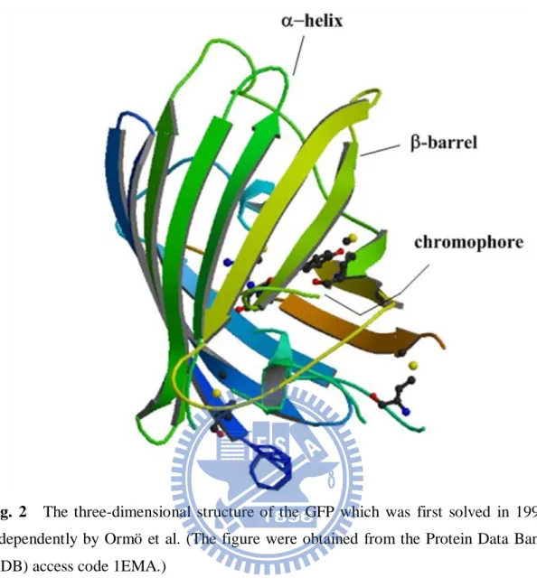
Fig. 2 The three-dimensional structure of the GFP which was first solved in 1996 independently by Ormö et al. (The figure were obtained from the Protein Data Bank (PDB) access code 1EMA.)
The GFP consists of 238 amino acids and its crystal structure is an 11-stranded
β-barrel [5, 6]. The Fig. 2 shows the first crystal structure until they have been
reported for tens of years. The chromophore is derived from only a few important amino acids which are located near the center of the β-barrel. It is
p-hydroxybenzylidene -imidazolinone (p-HBDI, see Scheme 1) formed from
tripeptide serine-65 (Ser65), tyrosin-66 (Tyr66), and glycine-67 (Gly67) in the native protein for the primary structure [7-9].
4
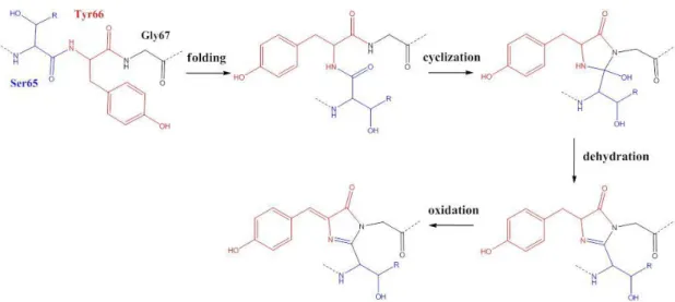
Fig. 3 The biosynthetic mechanism for the formation of the GFP chromophore.
Fig. 3 shows the mechanism begins by a nucleophilic attack of Gly67 on the carbonyl group of Ser65 to form a five-membered ring after the denatured GFP’s folding. Then the reaction followed by loss of H2O after the cyclization. The final step
is the oxidation of the hydroxybenzyl side chain off Tyr66 [10].
Fig. 4 Oxidation of Tyr66 leads into forming two fluorescent states – the neutral (protonated) and anionic (deprotonated) species.
The GFP variants may be divided into several classes based on the distinctive of their chromophores. There are wild-type mixture of neutral phenol, anionic phenolate, phenolate anion, and so on. The wild-type GFP (wt-GFP) has two characteristic absorption bands at room-temperature. One is a major excitation peak at 395 nm and another minor peak at 475 nm. When excitation is at about 395 nm that gives emission is at 508 nm [2, 9, 11]. Fig. 4 represents the neutral and anionic forms which
5
may be responsible for the 395 nm and 475 nm excitation peaks, respectively. The equilibrium between these two forms is influence by external factors like temperature, PH, and the environment of the protein [6, 10]. The excited states of phenols are much more acidic than their ground states, so that the emission would occur only from the deprotonated species [9, 12].
Chattoraj and co-workers demonstrate that the neutral form can be converted to the anionic form by excited-state proton transfer. The room-temperature (298K) and 77K electronic absorption spectra of the GFP are much more different from Chattoraj’s ultra-fast excited dynamic results [12-14].
Scheme 1
Martin calculate the fluorescent path for the anionic HBI (Scheme 1) of the GFP by using the Complete Active Space Self-Consistent Field (CASSCF) level of theory with the 6-31G(d) basis set and the active space for 12 electrons in 11 orbitals [15].
6
emission spectra compared with the protein environment [16], ultrafast polarization spectroscopy for internal conversion process and excited-state-proton-transfer reaction [17, 18], temperature dependence and isoviscosity analysis for the internal conversion of the GFP chromophore [19].
DsRed is a recently cloned red fluorescent protein from Discosoma coralby the homology to the GFP. Like the formation of the GFP, the chromophore in DsRed is also formed by the intramolecular reaction of the three amino acids which is glutamine-66 (Gln66), tyrosin-67 (Tyr67), and glycine-68 (Gly68) (HBMPI, see Scheme 1)[20]. Both the GFP and DsRed chromophores share the same 4-hydroxybenzylidene-imidazolinone core, but they differ from the linkage at the imidazolinone ring. The more extended conjugated Π-system in the chromophore may cause the significant red shift of the DsRed absorption properties compared to those of GFP [21, 22].
In the present work, we investigate three GFP chromophore structures and one DsRed chromophore structure which are shown in scheme 1. There have been numerous studies for the equilibrium geometries of ground state and excited states. So we optimize the ground state, namely S0 and the first-singlet-excited-state, namely S1.
First of all, discussions of the symmetry are very important. From the following theory which will demonstrate the principle for absorption and fluorescence spectra
Then, we compare the S0 vibrational frequencies calculation with the experiments
of Infrared (IR) spectra in order to demonstrate what the S0 geometry is [23]. We
would also compare the vibrational frequencies of S0 with S1. That means if the
vibrational normal modes are similar in these two electronic states, the simulation of the absorption spectra could base on the displaced harmonic oscillator approximation [24]. Finally, we will simulate the absorption and fluorescence spectra using ab initio methods and also the solvent effects will be taken into account for the simulations.
7
Chapter 2 Theory
2.1 Density Functional Theory (DFT)
The first idea of describing the atomic and molecular systems as a functional of the electron density ρ(r) started with Thomas-Fermi model rather than the wavefunction [25]. In their quantum statistical model, a uniform electron gas, only the kinetic energy (the 1st term, T) was considered but it is a very coarse approximation to the true kinetic energy. The nuclear-electron (the 2nd term, Ene) and electron-electron (the
3rd term, Eee) contributions were treated as a classical way without any effects of
exchange and correlation. The Thomas-Fermi energy expression is shown as
2 / 3 1 2 2 5 / 3 TF 1 2 123
1
E
3
10
2
2.1
r
r
r
ρ
r dr Z
dr
dr dr
r
r
Inclusion of the quantum mechanical exchange part for Eq. (2.1) is given the Thomas-Fermi-Dirac expression as
1/ 3 4 / 3
TFD TF3 3
E
E
2 2
4
ρ
ρ
r dr
.
Unfortunately, the Thomas-Fermi-Dirac model does not achieve success in chemical applications just like the Thomas-Fermi model. But their points of view really play an important role for the development which is commonly called density functional theory (DFT).
The first Hohenberg-Kohn theorem states that the external potential Vext (r) is (to
within a constant) a unique functional of ρ(r) [26]. The ground state electronic energy is uniquely determined by the one-electron density. Thus, all the properties of the states are formally determined by the functional of the ground state electron density. The other Hohenberg-Kohn theorem states the functional that is satisfied with the
8
variational principle. It delivers the lowest energy for the ground state of the system only if the trial density is exactly the true ground state density. The simple equation can be expressed as [27]
ne
ee
0
0
E
ρ
T
ρ
E
ρ
E
ρ
E
ρ
2 3
.
The success of the DFT methods is based on the ingenious idea by Kohn and Sham in 1965 who is finding a better way for the determination of the kinetic energy [28]. Kohn realized that Hartree equation gave the better description for atomic ground states than Thomas-Fermi theory. The difference between these two theories is the treatment of the kinetic energy. Thus Kohn and Sham presented the concept of a non-interacting system moving under the influence of the effective external potential (Veff,Eq.(2.4)) corresponding to the electron density. They suggested the Hartree Fockmethod and obtained the wavefunction of the exact kinetic energy in non-interacting system [29].
eff ext xcV
r
V
r
V
r
V
r
2.4
2 S1
T
2.5
2
N i i i
But this kind of expression is not equivalent to the true kinetic energy of non-interacting system. So they applied for exchange-correlation energy (Exc) in the
Kohn-Sham formulation. The ground state energy is given by
DFT S ne xc 1 2 2 ext 1 2 12E
T
E
J
E
1
1
2
2
r
r dr 2.6
N i i i xcρ
ρ
ρ
ρ
ρ
r
r
r
r dr
dr dr
r
e
T
T
E
J
r
r
d
r
2.7
E
xcρ
ρ
Sρ
eeρ
ρ
e
xc
9
where the exc term in Eq. (2.6) and (2.7)represents the exchange-correlation energy per particle. Besides, there are numerous approximations for Exc in order to improve
the accuracy.
The Local Density Approximation (LDA) is the simplest assumption that the density varies with the position slowly as the following equation [30, 31].
e
r
r
d
r
2.8
E
LDAxcρ
xc
where the exc term in Eq. (2.8) represents the exchange-correlation energy per particle of a uniform electron gas of the density. LDA gives the extremely useful results for other applications. The Local Spin-Density Approxition (LSDA) is the extension of LDA to the unrestricted system.
,
e
r
,
r
r
d
r
2.9
E
LSDAxcρ
ρ
xcρ
ρ
Furthermore, in order to improve the accuracy of the non-uniform of the true electron density, the generalized gradient approximation (GGA) includes both electron density and its gradient of the density
r . The expression can be simply defined as
,
f
r , r ,
r ,
r
dr
2.10
EGGAxc ρ ρ
ρ ρ ρ ρ When the extension takes higher order gradient of electron density into account, it is called meta-GGA method.
A number of hybrid functionals, which use the exact exchange energy is given by Hartree-Fock theory. This strategy performs accurate exchange-correlation energy. The most popular hybrid functional, B3LYP, expressed the exchange-correlation energy as [32]
1
E
E
E
1
E
E
(2.11)
E
B3LYPxc
a
xLSDA
a
exactx
b
xB88
c
cLSDA
c
LYPc10
experimental data with values of 0.2, 0.72, and 0.81, respectively. For the B3LYP-35 functional, the values are 0.35, 0.585, and 0.81, respectively. For the BHandHLYP functional (Note that this is not the same as the “half-and-half” functional reported by Becke), the values are 0.5, 0.5, and 1, respectively. Much current work is still concerned about developing to improve the accurate exchange-correlation functionals.
The advantages of DFT, especially those involving gradient corrections and hybrid methods, have a significant improvement in the accuracy. However, DFT can be used to study larger molecules than other ab initio methods.
2.2 Time-Dependent Density Functional Theory (TD-DFT)
The successful treatment of DFT has inspired the theorists to develop many applications. However, the Hohenberg-Kohn-Sham formulation of DFT is time-independent treatment, thus it could not be demonstrated for arbitrary systems involving time-dependent problems such as molecular optics, absorption, fluorescence, nonradiative processes, and so on.
Therefore, time-dependent DFT (TD-DFT) is based on the Runge-Gross theorem just as DFT is based on Hohenberg-Kohn-Sham theorem [33, 34]. They specified an initial state Φ
t0 at t = t0 and density n
r,t
obtained from a many-body system with
Hamiltonian Ĥ. They supposed the time-dependent Schrödinger equation of a many-body system can be solved.
ˆ ˆ
ˆ
2.12
ˆ ee V t ext V T t H where Tˆ is the kinetic energy, Vˆext t is the time-dependent potential, and the Vˆee
11
r
,
t
t
n
ˆ
r
t
2.13
n
with ˆ
S
S S n r r r
, where s represents spin variable. At first, they
demonstrated several important theorems before constructing the time-dependent Kohn-Sham Schrödinger equation.
The exact time-dependent density of the system can be computed from
,
,
,
2.14
2
1
2t
r
t
i
t
r
t
r
V
eff
j
j
andn r t
,
j
r t
,
jr t
,
2.15
where the exact density of the system can be obtained from single-particle orbitals
r,t j
with one-particle potential Veff
r,t .The hard work for time-dependent system is that it could not be based on the usual variational principle. Recently, due to the accuracy of the calculation, TD-DFT has replaced the single-excitation configuration interaction (CIS) which based on HF theory.
2.3 The Brief Polarizable Continuum Model (PCM) Method
So far, we only talk about the stationary-state quantum mechanics of an isolated molecule. But most of chemical reactions occur in the solutions that those solvents play an important role on the molecular properties like equilibrium structure, vibrational frequency, and so on.
For a continuum solvation model, the solvent generates a reaction field which is considered as a continuous dielectric and the solute is treated in a molecular cavity of realistic molecular shape. The interaction between the solute and the solvent may be
12
calculated by self-consistent reaction field method (SCRF) [35, 36].
Among several versions of polarizable continuum model (PCM) methods, integral equation formalism PCM (IEFPCM) method is a widely generalization of PCM applications for isotropic dielectrics, anisotropic dielectrics such as liquid crystals and polymers, and so on [37, 38].
2.4 Principles for
Absorption and Fluorescence Spectra
In most molecular systems, the Born-Oppenheimer (B-O) approximation is very important for the theoretical treatment of molecular processes. The Franck-Condon overlap integrals of the two electronic states are essential for the vibronic structure of electronic spectra such as absorption spectra, fluorescence spectra, electronic transfer, and so on.
The quantum mechanical expression for the absorption coefficient is based on the time-dependent perturbation method and dipole approximation. The absorption coefficient for molecular systems in dense media can be expressed as [39]
2 D
2.16
3 4 , ' 2 ' ' 2
bv av bv av v v av P ba c a where ba is the electronic transition dipole moment, P is the Boltzmann factor, av
2 ' av bv
represents theFranck-Condon factor , and the factor a is introduced to
take into account the solvent effect. If the dephasing (or damping) effect is included, the Lorentzian lineshap function can be presented as the following relation.
2.17
2
1
1
D
,' 2 2 ,' ,'
it t ba av bv ba av bv ba av bvdte
13
j j j ba av bvv
v
2
.
18
2
1
2
1
'
,'
where r is the so-called dephasing (or damping) constant. ba ba denotes the electronic energy difference between the two electronic state a and b at the
equilibrium geometry. The relation is presented as ba
EbEa
1
.
The wavefunction of harmonic oscillator is expanded into the product of each vibrational mode in Eq. (2.19) and Eq. (2.20). av
Qjj
and bvj
Qj denote thevibrational wavefunctions of the j-th normal-mode for an initial electronic state a
and a final electronic state b , respectively.
2.20
2.19
j v b j v b j av j av
Q
Q
Q
Q
j j
where Qj is mass weighted normal-mode coordinates including both intra- and intermolecular vibrations. Within displaced harmonic approximation, the previous absorption coefficient expression can be derived as
2
exp
2.21
3
2
j j ba bat
G
t
it
dt
ba
c
a
And the time correlation function Gj
t is expressed as
2.22
2
1
2
1
exp
2
bv av j j j v v av jt
P
it
v
v
G
j j j j j
After simplifying, Gj
t can be rewritten as
exp
2
1
1
j it j
2.23
j it j j j jt
S
n
n
e
n
e
G
14
where nj is the phonon distribution
1
1
kT j B je
n
and Sj is usuallycalled the Huang-Rhys factor 2
2 j j j d S
. In the Huang-Rhys factor expression, j is the harmonic frequency of the j-th normal-mode and dj is the displacement between the initial and final electronic state. The Huang-Rhys factors can give some information of spectra before the simulation. The Huang-Rhys factor Sj< 1 means weak coupling. On the other hand, Sj >> 1 means strong coupling.
Finally, the absorption coefficient of displaced harmonic oscillator is analytically derived as
2
1
1
2.24
exp
2
3
2
j it j it j j j ba ba j je
n
e
n
n
S
t
it
dt
ba
c
a
For the cases of harmonic oscillator at T = 0 K, we can easily determine the Franck-Condon factor as Eq. (2.25).
2.25
!
2 0 j j j j S j v j a v be
v
S
And the absorption coefficient is
2.26
1
exp
2
3
2
0 ,
j it j ba a v b je
S
t
it
dt
ba
c
a
where ba 1
Eb Ea
0 .For displaced harmonic oscillators, the absorption and fluorescence spectra show the mirror image relation which is due to the same transitions for invariant
15
Franck-Condon factor. The fluorescence coefficient is shown in Eq. (2.27).
2
D
2.27
3
4
, 2 ' 2
bv
av bvav
v v avP
ba
c
a
I
Following the similar procedures as above, then the fluorescence coefficient of displaced harmonic oscillator is analytically derived as
2
1
1
2.28
exp
2
3
2
j it j it j j j ba ba j je
n
e
n
n
S
t
it
dt
ba
c
a
I
where ba 1
Eb Ea
0 .If the molecules are dissolved in the solvents, the solution environments are in disorder that caused the inhomogeneous phenomenon. For practical applications of solvent effect, the effects of inhomogeneity are taken into account. Suppose that the
effects of inhomogeneity are associated with the electronic energy gap ba. The Gaussian distribution function of inhomogeneities can be defined as
1
exp
2
2.29
2 2
ba ba ba ba baD
D
N
where ba denotes the average energy gap and Dba is the width of the distribution. Then
2.30
4
exp
2 2
t
D
it
e
N
d
e
ba ba it ba ba itba
ba
Finally, the absorption coefficient of displaced harmonic oscillator with inhomogeneity is derived as
16
2
1
1
2.31
4
exp
2
3
2
2 2
j it j it j j j ba ba ba j je
n
e
n
n
S
t
t
D
it
dt
ba
c
a
For the treatment of displaced anharmonic oscillator, the harmonic wavefunction will be utilized as a basis and the anharmonicity is considered as a perturbation [24]. Using the perturbation method to expand the j-th vibrational normal-mode potential as
j2 2j
j3 3j
2 j4 4j
2.32
j
Q
a
Q
a
Q
a
Q
V
in which is chosen as the perturbation parameter. The following presents the expansion of the wavefunction.
0
1
2 2
2.33
v j v j v j j vjQ
jQ
jQ
jQ
where v
Qj j 0
denote the zeroth-order harmonic wavefunction. The first-order correction to the wavefunction is
3/ 2 3 3 1 0 3 0 1 1 0 0 3 3 3 1 2 1 1 2 3 1 2 3 j v j j v j j v j j j j j j v j j j j v j j j j j j a Q v Q v Q v v v Q v v v Q
2.34
We only consider the first-order anharmonic correction to the wavefunction which is based on the displaced harmonic oscillator. The second-order and the higher-order correction will be neglected due to the fewer contributions.
Finally, the absorption coefficient within the displaced anharmonic oscillator of the first-order correction is analytically derived as
![Fig. 1 The bioluminescent organ is located along the umbrella-like edge [1].](https://thumb-ap.123doks.com/thumbv2/9libinfo/8247681.171577/19.892.134.758.536.1105/fig-bioluminescent-organ-located-umbrella-like-edge.webp)
![Table 4 X-ray crystal structure from Ref. [46].](https://thumb-ap.123doks.com/thumbv2/9libinfo/8247681.171577/52.892.127.767.128.1083/table-x-ray-crystal-structure-ref.webp)