Predictive adaptive control system for unmeasured disturbances

Subscriber access provided by NATIONAL TAIWAN UNIV

Industrial & Engineering Chemistry Process Design and Development is published by the American Chemical Society. 1155 Sixteenth Street N.W., Washington, DC 20036

Predictive adaptive control system for unmeasured disturbances

Hsiao Ping Huang, Yung Cheng Chao, and Pea Hsien Liu

Ind. Eng. Chem. Process Des. Dev., 1985, 24 (3), 666-673 • DOI: 10.1021/i200030a023 Downloaded from http://pubs.acs.org on November 18, 2008

More About This Article

The permalink http://dx.doi.org/10.1021/i200030a023 provides access to: • Links to articles and content related to this article

Predictive Adaptive

Control

System for Unmeasured Disturbances

Hslao-Plng Huang,'+ Yung-Chong Chao, and Poa-tldon Llu

Depa-nt of Chemical EnglmMng, Natbnai Taiwan University. Taipei, Taiwan, R.O.C.

The algorithms for the estimation, predlctlon, and compensation for unmeasured disturbances are considered in

a predictive adapthre control (PAC)

system.

According to an identifled dynamic model for the process, an q h a l e n t

unmeasured disturbance is flrst estlmeted. Then, the estimated dlstwbences are fitted Into a difference equation

by means of theHn6arregresslon. Owingtothe nonstatkner#ykwrdencyof the ummrasueddistubances, an orbline

exponential data window is used to update the regression model. Subsequentty, a predlctlve compensation is made

by making use of the resulting regression model and the system dynamlc model in a feedforward manner and is

accompanied by a feedback control loop. Simulations show that the PAC system is superior to a simple feedback

control system whlch is already tuned optimally. It should be mentioned that the identification of the process

dynamic model In the knplementation of the PAC can be conducted with closed-loop data and the algorithms In

the PAC are good for real-time Implementation.

Introduction

The existence of unmeasured disturbances

w

i

l

l

usually

result in some defects in a control system deaign. Although

a feedback control system, conventional or optimal, can

usually recover from those unknown inputs, the perform- ance of the control system is degraded. Thus, a better approach of control is always desirable. The earliest study

on the control of the unmeasured disturbance is, perhaps,

the work of Johnson (1968).

It

concluded that through a

proper choice of the quadratic performance index, an op-

timal control can be implemented by a proportional plus

integral feedback control principle. Later, the designs of the state observers for the systems where unpeasured

disturbances exist are investigated by Johnson (1975) and

by Meditch and Hostetter (1974). Recently, the unmea- sured disturbances together with the unmeasured state were considered in a design of the inferential control system by Joseph and Brosilow (1978a,b,c), Morari and

Stephanopoulous (1980), and Morari and Fung (1982). In

those studies mentioned, it is assumed that the dynamics

between the unmeasured disturbances and the state var- iables of the system are well defined. However, in the practical situation, very often, the dynamics must be modeled through identification procedures and thus there

seems to be no way

to

underatand the dynamics for those

unmeasured disturbances. On the other hand, the models used in control designs are usually good for some specific

conditions only, owing to the nonlinearity and complexity

of the chemical processes. Thus, in an ever-changing circumstance, where the system parameters or operation

conditions vary from time to time, the resulting systems

based on the given model

will

be defective. One approach

to solve the problem mentioned is

to

continually identify

the process on-line. Although some on-line identification algorithms are available in the literature (for example, Saridis, 1974; Isermann et al., 1974; Huang and Chao, 1982), the process usually has to be interrupted from its normal operational conditions. The interruption is con- ducted either by sequentially switching the form of the regulator from one to the other (Gustavsson et al., 1974)

or by introducing some special inputs. Most of these ?rinds

of interruption are strongly undesirable in chemical plants. The other approach is to keep the nominal model un-

Address after August, 1985: Department of Chemical En- gineering, Room 66-469, Massachusetts Institute of Technology, Cambridge, MA 02139.

changed and lump

all

the unknown inputs and the effects

of modeling errors into an equivalent unmeasured dis- turbance. The compensation for this unmeasured dis-

turbance can then be conductad with a feedforward scheme if the unmeasured disturbance is estimated on-line. Au- thors such as Garcia and Morari (1982), Liou and Hsu (1983a,b), Tong (1982), and Liu (1983) discussed the control of the unmeasured disturbance recently. Among these, Tong (1982) and Liu (1983) considered the esti- mation of the lumped unmeasured disturbance by use of

an identified nominal model. Owing to the time delay in

the process, a zero-order or a fiist-order extrapolation for

the unmeasured disturbance used by most of these authors

is not satisfactory for the control implementations. Be-

sides, the noises that may accompany the outputs will have

serioue effects on the system proposed by Liou and Hsu (1983b).

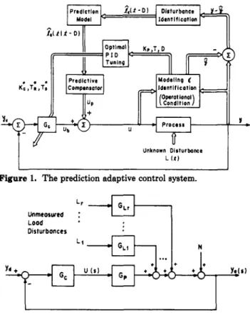
In this paper, a predictive adaptive control system as shown in Figure 1 is proposed. In this proposed system, a dynamic model is identified by the data from a closed- loop control operation. Later, any discrepency between the response of the model and that of the process is con- sidered a lumped effect of an equivalent unmeasured disturbance. This unmeasured disturbance can be iden-

tified by a real-time algorithm. A real-time prediction

model for the unmeasured disturbance is then identified and is used to predict the disturbance that is needed in computing a delayed compensation. The compensation is arranged as a feedforward control and is appended to a feedback control loop, either a conventional or optimal state feedback one. In this manner, the system possesses the capacity for compensating for the unmeasured dis-

turbance as well as the model errora that may exist. The

results of a series of digital simulations show that the system is superior to the simple feedback one which is tuned optimally.

The Estimation and Prediction of the Unmeasured Disturbances

Consider a single-loop control system in Figure 2, where a number of different unmeasured disturbances exist.

Because the distubances are either unmeasurable or un-

known, their transfer functions to the output will not be available. However, the transfer function from the ma-

nipulation input, i.e., G,(s), can be identified during a

transient period of a feedback operation by the method proposed by Huang and Chao (1982). Some descriptions of the modeling procedures are summarized in the Ap- 0 1985 American Chemical Society

Ind. Eng. Chem. Process Des. Dev., Vol. 24, No. 3, 1985 687

6 can be found elsewhere, for example, Huang and Chao

(1983) and Reid (1983). The index

k

denotes the value of

each variable at the instant of kth sample interval from the origin.

It is assumed that the value of the unmeasured dis-

turbance being estimated at instant

k,

denoted as l,(k

-

d), results from a constant input which lasts for a period

of N sample intervals. Thus, the estimated value of I,(k

-

d ) can be obtained through an averaging filter as Prediction Model II II

-

II Unknown D i s t u r b n c e L I t )

I

Figure 1. The prediction adaptive control system.

Unmcorurcd :

Dirturbonccs

Yds,

Figure 2. Block diagram for the control system with unmeasured disturbance.

pendix. According to the model thus obtained, the un- measured disturbances in Figure 2 can be considered a lumped equivalent disturbance as

r

i = l

Y ( S ) = Gp(s)u(s)

+

CG,i(s)Li(s)

= G p ( s ) [ u ( s )

+

Le(s)l (1)

where

According to the modeling procedures (Huang and Chao,

1982), a dynamic equation of G p of a first order with delay

or a second order with delay will result. Thus, a time

domain equation equivalent by eq 1 will be

p(t)

+

a&) = b,u(t

-

D)

+

Z,(t

-

D)

(3)

jqt)

+

a1Y(t)

+

a,y(t) = bou(t -

D)

+

Z,(t

-

D)

(4)

where, 1, is the equivgent unmeasured disturbance to the

system. If the observed process output is denoted 4s yo,

where

(5)

it is usually assumed that e ( t ) is a normally and inde- pendently distributed random variable.

Equations 3 and 4 can be transformed into their equivalent sampled-data equation

or

Yo = Y ( t )

+

4 )

Yo&) = dlYo(k

-

1)

+

d,yo(k

-

2)

+

f , u ( k

-

d

-

1)

+

f + ( k

-

d

-

2)

+

gil,(k

-

d

-

1)

+

g,l,(k - d

-

2)

+

((k)

(6)

(7) Computation methods for evaluating the Coefficients in eq where

((k)

= e(k)

-

&€(k

-

1)

-

42e(k

-

2)

where

i 2

and N’equals N

-

1 as eq 3 is used or N’equals N

-

2 as

eq 4 is used.

It is expected that through a proper choice of N, the value of Z,(k

-

d ) will approach

j)1)/(91

+

g2) (10) which corresponds to $hat in the case of noise-free at the output.

If a moving rec- data window of length N is used,

a recursive estimate of 1, can be formulated as

1

N

i,(k

-

d ) = I,(k - d

-

1)

+

,[6,

-

bk-N!] ₍₁₁₎

Thus, a t instant

k

and according to the definition pf 1,

in eq 3 and 4, only the value of l,(k - d ) rather than I,&)

will be obtained. It can be found, later, that a prediction

value of the unmeasured disturbance, denoted p I,(k/k

d), using all the available information, such as Z,(k - d),

Z,(k

-

d

-

11,

...,

is required for computing a feedforward compensation a t the kth instant.

By the definition of eq 2, the unmeasured disturbance can be consid_erecl a dynamic process. To enhance the prediction of l , ( k / k - d ) , a dynamic model for this un-

measured disturbance is desirable. In the many studies of the dynamic systems with unknown and inaccessible inputs, it is usually assumed that the unknown input can be formulated as a linear dynamic equations with some sparsely populated sequences of completely unknown im- pulses (Johnson, 1975; Meditch and Hostetter, 1974; Davison, 1972, etc.) or step inputs (Johnson, 1968). Thus, it is reasonable to assume that the increment of the un- measured disturbance betweeh each sample instant, i.e. (12) can be formulated as a difference equation with a proper order, i.e.

uo‘) =

ieo’)

-

ieo‘

- 1)

U G

+

1) = h 1 ~ G )

+

h+G

-

1)

+

... +

~ , u ( J ’ - s

+

1) (13)

Thus the coefficients in eq 13 can be found by using a regression model

uo’

+

1) =

&uG)

+

h2u(j - 1)

+

...

+

h8uG

- s

+

1)

+

eG) (14)

=

PVO)

+

e G )

6

=

[hl, h2,

...,

&IT

Vg’) = [ u ( ), ug’ - l),

...,

uo’ - s

+

1)]T and

The values of h can be calculated by a linear leastisquare

algorithm which minimizes the sum of m squared errors,

i.e., Cj”ple2g’). As the dypamic model in eq 13 may be

time-varying, the value of h

,

must be calculated from time

to time in accordance with the changing environment of the system. A recursive algorithm with a forgttting factor

a is adopted for the real-time estimation of h

.

This up-

dating algorithm is also given in the Appendix.

From eq 14 the prediction value for Og’

+

l/j) will be

(15)

Og’

+

l/j) = hlUg’)

+

h2UG

-

1)

+

...

+

fi,ug’ - s

+

1)

so that, for m 5 s

00’

+

m / j ) =

h,00:

+

m - l/j)

+

...

+

h,u(j)

+

and, for m

>

s

fig’

+

m / j ) =

&OG

+

m - l/j)

+

f 2 f i ~

+

m - 2 / j )

+

...

+

h,Og’

+

m - s / j ) (17)

Because of eq 15,Og’

+

m / j ) can be expressed in terms of

ug’), ug‘ - I),

...,

and ug’ - s

+

1); for example

OQ

+

2 / j ) =

h,+lug’ - 1)

+

... +

&ug‘

+

m- s) (16)

hlcg’

+

i/j)

+

h2ug’)

+

h3ug‘

-

1)

+

...

+

~ , U G

-

s

+

2) - 2)

+

...

+

(hlh,-l

+

h,)ug’ - s

+

2)

+

h1h,Uo’- s

+

1) = (h12

+

&,)ug‘),+l(h,&,

,+

h,)ug’ - 1)

+

(&

+

h,)ug’

= q 1 ( 2 ) ~ ( j )

+

Q , ( ~ ) u ~ ’ - 1)

+

...

+

q , ( 2 ) ~ ( j - s

+

1) (18) The same procedures can be carried out to the following result

Og’

+

m / j ) =

with

q l ( m ) u g ’ )

+

q2(m)ug‘

-

1)

+

...

+

q*(m)uO‘ - s

+

1) (19)

qi(m) = [A”.C]; (20)

where,

[ I i

denotes the ith component of a vector in the

parentheses, and A =

1.

;;

!:::

1

( 2 1 ) h t S . 1 ,

o . . .

c

= [l, 0 ,

...

O]T h,, 0 0 0 “ ‘ 0 and (22) Finally d i = l j , ( k / k - d ) = CO(k - d

+

i / k

-

d )

+

i e ( k - d ) = & q i o ( k - d - i

+

1.)

+

te(k -- d ) (23) i=l where qi = qi(1)

+

...

+

?p

(24)

In order to test the algorithm given above, a system as

shown in Figure 3 is used as the example for digital sim-

L e ( t h e unmeasured disturbance 1

I

I

Figure 3. Block diagram for the control system with lumped dis- turbance. 0 0 150

J

L 11) 1. ( f - D I % ( ~ I I - c J )

-

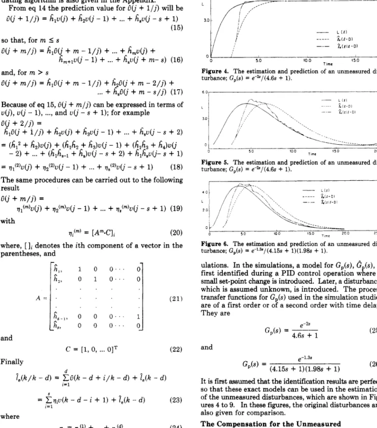
_ _ _ _ . l o o Time 50

Figure 4. The estimation and prediction of an unmeasured dis- turbance; G,(s) = e-&/(4.6s

+

1).

E n

--

” - 1 I

Figure 5. The estimation and prediction of an unmeasured dis- turbance; G,(s) = e-%/(4.6s

+

1).

Figure 6. The estimation and prediction of an unmeasured dis- turbance; GJs) = e-l,”/(4.15s

+

1)(1.98s

+

1).

ulations. In the simulations, a model for G,(s), G (s), is

first identified during a PID control operation wkere a small set-point change is introduced. Later, a disturbance, which is assumed unknown, is introduced. The process

transfer functions for G,(s) used in the simulation studies

are of a first order or of a second order with time delay. They are “-2s C,(S) = -E-.-- 4.6s

+

1 (25) and ,-1.3s (26) Gp(s) = (4.15s

+

;)(1.98s

+

1)

It is first assumed that the identification results are perfect so that these exact models can be used in the estimation of the unmeasured disturbances, which are shown in Fig-

ures 4 to 9. In these figures, the original disturbances are

also given for comparison.

The Compensation for the Unmeasured Disturbances

Although a conventional feedback control system will, in general, alleviate the effect of external disturbances, it

Ind. Eng. Chem. Process Des. Dev., Vol. 24, No. 3, 1985 660

6 0 1 1 _or

boup(t)

+

blUP(t) = - i e ( t / t

-

D)

(28)

In the case where bl is zero, eq 27 and 28 become

(29)

where, up(t) denotes the predictive feedforward input for

the unmeasured disturbance.

In a sampled-data system, the predictive feedforward control input is given from eq 6 as

1 -

up@) = --Ze(t/t

-

D)

bo

up(k) =

--V2up(k

-

1)

+

glie(k/k

-

d )

+

gJe(k

-

l / k

-

d ) ) (30)

fl

There are many reasons that the predictive feedforward

control, up, cannot stand alone to compensate for the un-

measured input. Thus, up must be appended with a

feedback loop. The feedback input may be of a conven- tional PID control, denoted as ub, or of an optimal state

control, (OSC) denoted as u,. Thus, the overall control

input denoted as u will be

u = up

+

ub (or up

+

u,) (31)

The sampled-data algorithm for the ub in the following 1 studies is given as 6 U b ( k ) = U b ( k

-

1)

+

k,-W(k)

+

k,[w(k) - W ( k - I)] TR (32) where

-

L.1' , 50 I 5 0 20 0 'O0 Time -6Ob

Figure 7. The estimation and prediction of an unmeasured dis- turbance; G,(s) = e-'.%/(4.15~

+

1)(1.986

+

1).

7

---I-

Identif ication of Oynomic Model from Closed Loo(

I

First Phase

Prediction

Second Phase

Figure 8. The flow chart for the implementation of the PAC.

t

i

-

0.4

0 50 _{too Time} 150 200

Figure 9. The responses of the PAC and the conventional PID system subjected to an unmeasured disturbance; example 1.

is still desirable to compensate for those measurable dis-

turbances in a feedforward manner so as to reduce errors.

The efforts on the feedforward control have been initiated and developed during the past 20 years. Examples of work in this area are provided by Ballinger and Lamb (1962),

Cadman et al. (1967), Luyben (1963), and Huang (1969).

As

described in the previous section, through the estima-

tion and prediction procedures, the unmeasured loads can be considered as if they were measurable. Thus, the feedforward compensation becomes feasible. However, as mentioned in most of the literature about feedforward control, a feedback loop is indispensable. According to the dynamic models in eq 3 and 4, a feedforward compensation of the unmeasured disturbance can be given as

boup(t) =

- l e ( t / t -

D)

(27)

I D

W ( k ) = w(k - 1)

+

-

[e&)- e(k

-

l)]

+

CXTD

+

6

Equation 32 corresponds to an interactive analog PID control algorithm.

The optimal state control input, uo, in this study starts

with the state equation for eq 6 where t ( k ) is assumed as

zero, i.e. (33) and ~ ( k

+

1) = H,x(k)

+

H2u(k - d ) Y(k) = c d k ) x(k) = [Xl(k), X2(k)lT where and H2 = vi,

fzlT

c = [l, 01 (34)

so that u,(lz) is given as

u,(k) = [433ldI(1)m

+

[KHldl(2)42.Y(k

-

1)

+

KH+,(k

-

1)

+

KH1H2uO(k

-

2)

+

...

+

KH,d-lHzu,(k

-

d )

+

[KHld](2)f2u(k

-

d

-

1) (35)

where

[la)

denotes the ith column of the matrix in the

parentheses. The gain for the state feedback, K, is ob- tained by minimizing a quadratic performance index

I.P. =

2

[ Q y ( k ) 2

+

Ru(k)'] (36) The resulting system that uses eq 31 &s the control strategy

is considered as a predictive adaptive control system, PAC.

Stability Considerations of the PAC

The stability of the PAC system can be analyzed by examining the characteristic equation of the system. The following derivations are based on a second-order process which is the typical model for the dynamics of chemical processes.

k = O

According to eq 8, le(k

-

d ) can be written as

(flBd+l

+

f2Bd+2)u(k)) (37)

where B is a backward shift operator so that BkX(i) stands

for X(i - k ) . Let

" and and 8 Q2(B) = 1

-

R2(B)[1

+

CviB'(1

-

B)IPz(B) (48) i = l

Substitution of eq 46 into the dynamic equation of the process yields

{(I

-

41B

-

4zB2)Q2(B) - (figd+'

+

fzBd+2)Q1(B)I~(k) =

0 (49)

Thus, the characteristic equation of the system is (1

-

4iB

-

(PzB2)Qz(B)

-

Vi

+

fzB)Bd+lQ1(B) = 0 (50)

The stability of the system depends on whether all the zeros of eq 50 lie outside the unit circle of IBI = 1. It can be seen that the predictive feedforward control will affect the stability of the system in quite a complicated way. This is obviously different from the conventional feed- forward control for the measurable disturbance.

From eq 30 R z ( B ) is given as

One can conclude that for any bounded input le, the final

offset of the system will be

Thus, theoretically speaking, there is no need of an integral

action in R,(B). This fact will be very helpful for the

stability of the system. If the values of fl and f 2 are sig-

nificantly larger than those values of gl and g2 (this is the case where process gain is high), then the characteristic equation of eq 50 will approach that of a single feedback control system, i.e.

(1

-

&B

-

&B2) - (fl

+

f2B)Bd"R1(B) = 0 (56)

Thus, if an integral action is excluded from R l ( B ) , then

the closed-loop stability will be improved significantly, especially in the presence of the time delay.

Simulation Resplts for the PAC

In the followjng studies, implementation of the PAC as

shown in Figure 1 with different dynamic processes and disturbances are simulated via a digital computer. The implementation of the PAC consists of two phases. In the first phase, the system is operated by a conventional feedbackcontrol from which sufficient data are obtained to identify the dynamic model by the procedures given in Appendix. In the second phase, the dynamic model is considered invariant and the unmeasured disturbance is estimated and compensated. The flow diagram of the system implementation is shown in Figure 8.

In each of the following examples, the PID controller settings are obtained as follows. First, the dynamic equation of the identified model together with a PID

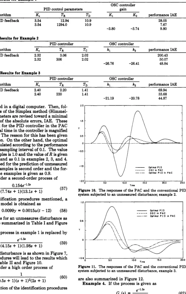
Ind. Eng. Chem. Process Des. Dev., Voi. 24, No. 3, 1985 671 Table I. Simulation Results for Example 1

OSC controller

PID control parameters gain

control algorithm KC TR TD K1 K 2 performance IAE

conventional PID feedback 3.54 12.94 10.9 28.06

PID in PAC 3.54 1294.0 10.9 7.67

OSC in PAC -3.80 -3.74 9.80

Table 11. Simulation Results for Example 2

PID controller OSC controller

control algorithm KC TR TC k l k2 performance IAE

conventional PID feedback 2.32 3.06 2.02 200.43

PID in PAC 2.32 306 2.02 50.07

OSC in PAC -26.76 -26.41 48.84

Table 111. Simulation Results for Example 9

PID controller OSC controller

control algorithm KC TR TD kl k2 performance IAE

conventional PID feedback 2.40 2.20 1.41 69.94

PID in PAC OSC in PAC

2.40 220

controller is simulated in a digital computer. Then, fol- lowing the procedures of the Simplex method (Himmel-

blau, 1972)) the parameters are revised toward a minimal

value of the integral of the absolute errors, IAE. These

settings are also used for the PID controller in the PAC

except that the integral time in the controller is magnified

with an order of

lo2.

The reason for this has been given

in the previous section. On the other hand, the optimal

state controller is calculated according to the performance

index in eq 36 with a sampling interval of 0.1. The value

of Q used in the examples is 1.0 and the value of

R

is given

as 0.75 in example 1 and as 0.1 in examples 2, 3, and 4.

The model of eq 13 used for the prediction of unmeasured

disturbance in the examples is second order and the for-

getting factor a in the examples is given as 0.9.

Example 1. Consider a second-order process of

(57) 0.154e-’.%

Gp(s) = (7.74s

+

1)(13.1s

+

1)

Through the identification procedures mentioned, a

differential equation model is obtained as

9

+

0.2069

+

0.0099~ 0.0015u(t

-

12) (58)

The simulation results for an unmeasures disturbance as

shown in Figure 5 are summarized in Table I and Figure

9.

Example 2. If the process in example 1 is replaced by

(59)

Gp(s) = (4.15s

+

1)(1.98s

+

1)

and the unmeasured disturbance is as shown in Figure

7,

then the similar procedures

will

lead to the results which

are summarized in Table I1 and Figure 10.

e-1.3S

Example 3. Consider a high order process of

(60)

Then, the implementation of the identification procedures results

4.079

+

3.679

+

y = ~ ( t

-

0.8) (61)

If the unmeasured disturbance is given as Figure 3, the

simulation results are summarized in Table I11 and Figure

11. The responses to the set-point change of the system

with the existence of the same unmeasured disturbance

1 (0.5s

+

l)(s

+

1)2(2s

+

1) G,(d = 1.41 33.68 -21.19 -20.78 44.87 1.5

t

n

I

-

O p I i m a i P I D O S C in P A C Optimal P I 0 in P A C ---_- I 50 10.0 15.0 2C.O 25.0 -25 Time

Figure 10. The responses of the PAC and the conventional PID system subjected to an Unmeasured disturbance; example 2.

0.6 . Y . 0 . 15.0 20.0 -0.6 I Time 0 5.0

Figure 11. The responses of the PAC and the conventional PID system subjected to an unmeasured disturbance, example 3.

are also summarized in Figure 12.

Example 4. If the process is given as e-1.2e

G,(s) =

-

(8s

+

1)

Instead, a model with biases in the parameters is assigned as

0.8e-l.%

2 . 5 [ I I I

₁

-

Optimol P I O

---

O S C in P A C --- P I 0 in P A C Y Tlme

Figure 12. The responses of the PAC and the conventional PID system subjected to an unmeasured disturbance and a set-point change; example 3.

0.6 I 1

₁

I

-

Optimol P 10 ( Bore on Biasod Model I

---

O S C in P A C (BoreOttBiaSedModcll

---

Optimal PI0 in PAC ( B O ~ on Bioud M0d.l I

I-

---

Optimal PI0 in PAC ( B O ~ on Exocf Model I

-0.6 1 I I I

0 5.0 (0.0 IS.0 20.0

TIM

Figure 13. The responses of the PAC and the conventional PID system subjected to an unmeasured disturbance; example 4. Table IV. Simulation Results for Example 4

PID controller

control algorithm K , Ta Tn ance

IAE

conventional PID feedback 4.34 7.975 0.54 58.49

PID in PAC 4.34 797.5 0.54 11.18

OSC in PAC 18.15

PID in PAC with exact model 4.59 645.45 0.54 9.51

The implementation of the PAC using the biased model

in the presence of some unmeasured disturbance is then

summarized in Table

Iv

and Figure 13. The result of the

PAC with the exact model is also given in the table for

comparison. From this table, it can be seen that the PAC is capable of compensating for the model errors as well as the unmeasured disturbance.

Summary

In the predictive adaptive control system as described in the text, the identification of models, estimation, and control of the unmeasured disturbance are considered an integrity. In practical situations where identification of the dynamic model cannot be repeated quite often, this system will provide the capacity for compensating for the unmeasured disturbances and model errors in an adaptive manner. From the analysis and simulations, the following conclusions are reached.

(1) The estimation, prediction, and control of the un-

measured disturbance in the PAC are all formulated as

real-time algorithms so that it is ready for an on-line im-

plementation. Initlol v o l u ~ r l o r lime deloy

1

Initial v o l u o for paromrterr On0 d h " r i o n

search tor time

Colculote 101-102 I02 Calculate I D 1 I I D 0 1 0 2 model Is resulted 1 st order modbl Is

0

resulted

Figure 14. The identification procedures for the process dynamic model.

(2) The prediction of the unmeasured disturbances, as shown in the examples, are superior to those of the zero- order or first-order extrapolation methods.

(3) The PAC system is more effective in compensating

for the unmeasured disturbances when compared with the

simple feedback control system which is tuned optimally.

(4) It seems feasible to append other dead-time com-

pensating feedback control to the predictive feedforward

control. Good performance can be expected from the re-

sulting system.

(5) From theoretical derivations, there seems to be no

need for an integral action in the appended feedback loop. In practice, a small integral action, as illustrated in the

examples, can be added so as to deal with the imperfection

of the estimations.

(6) The system is more favorable to those processes

whose process gain is high. In those cases, the system is

much easier to be kept stable than a conventional feedback

system.

Acknowledgment

This research is sponsored by the National Science Council of the Republic of China (NSC73-0402-E002-03).

Appendix

I. The Identification of the Dynamic Model for a

Process in a Closed Loop. The dynamic model used in the control system is obtained by means of identification procedures by Huang and Chao (1982). The procedures can be summarized in Figure 14.

The identification index (1.D.) used in Figure 14 is de-

fined as

I.D. = MSE/Det(H)I,. (A.1)

Ind. Eng. Chem. Process Des. Dev., Vol. 24, No. 3, 1985 873

f = coefficient in the discrete-time dynamic equation

g = coefficient in the discrete-time dynamic equation

6,

= continuous process transfer function

G, = identified process transfer function

GL = continuous transfer function for the disturbances

h = coefficient of a regression model in eq 14

h = a coefficient vector

HI, H2

7

a state expression for a second-order process

k = optimal state feedback gain

k , = the proportional gain of a PID controller

L = disturbance input

Le = the equivalent disturbance input

1, = the equivalent disturbance in time domain

Po)

= a jth iteration value of a s X s matrix

Q1, Q2 = polynomials of B defined in eq 47 and 48

R1 = the discrete-time transfer function for the feedback

Rz

= the discrete-time transfer function for the predictive

s = variable in Laplace transform

t = time

TR

= the integral time of a PID controller

TD

= the derivative time of a PID controller

u = the control input

up = the predictive feedforward control input

u, = the optimal state feedback control input

ub = the optimal PID control input

v = a difference quantity defined in eq 12

V = a column vector

w = a dummy variable in eq 32

y = the process output

yo = the observed process output

z = the variable in z transform

Greek Symbols

a = a forgetting factor in eq A.4 and A.5

6 = an error quantity defined in eq 9 or a sampling interval

t = observation error

9 = coefficient in the discrete-time dynamic model

[ = noise in the dynamic equation in terms of the observed

Literature Cited controller

feedback controller

in eq 32

output

Bolllnger, R. E.; Lamb, D. E. I n d . Eng. Chem. Fundem. 1962, 1, 245.

Cadman. T. W.: Rouths, R. R.; Kermcde, R. I. Chem. Eng. Pros. Symp. and

YP(P*) =

P *

where

MSE

is the mean squared error of the model being

considered. y is the output of the system, p

*

is the optimal

parameter vector for the candidate model, and tl,

...,

t N

are the N sampling instants.

The parameter estimation is implemented through an iteration algorithm of

P

-

Po

= [YpT(po)Yp(po)]-lYpT~o)[

Y

-

Y(po)] (A.3)

where Y ( p O ) is the output vector calculated at

P

= Po.

The starting value of p o can be found elsewhere (for ex-

ample, Liu, 1983).

11. The On-Line Algorithm for Updating the Re-

gression Model in Eq 14. A recursive algorithm with a

forgetting factor a is adopted for the real time estimation

of h in eq 14

60’

+

1) =

60’)

+

[a

+

xT0’

+

1)Po‘)xo’

+

1)]-1 x

P0’)xo’

+

l)[uo’

+

1) - XTo‘ +1)6o‘)1;

0’

1 m)

(A.4)

and

1

Po‘

+

1) = -{I

-

Po’)[,

+

XTo’

+

1)Po‘)xo‘

+

1)l-l x

CY

x(j

+

1)xTV

+

1))PG); (j L m) (A.5)

where

xG)

=

[uG),

UG

-

l),

...,

U G

-

s

+

1)IT (A.6) VG) = [uo’), dj - 11,

...,

v0’

-

m

+

1)IT (A.7)

The starting values of

6

(m) and p(m) for eq A.4 and A.5

6 ( m )

= [XT(m)X(m)]-lXT(m) V(m) (A.8) P(m) = [XT(m)X(m)]-l (A.9) are given by and where X(m) = [ Vg’ - I), V(j

-

2),

...,

V ( j

-

s)] (A.lO)

The value of m in eq A.8 and A.9 denotes the number of observations that is uzed in the least-squar calculation

for the initial value of d

.

Nomenclature

a = constant coefficient

A = an s X s matrix B = an s X 1 vector

b = constant coefficient

B = a backward shift operator

C = an s X 1 column vector

D = time delay

d = time delay in terms of sampling interval

e = error between the set-point and the observed output

- 1987, 6(3), 421.

Davlson, E. J. IEEE Trans. Autom. Control 1972, 17, 821.

Qarcla. C. E.; Morarl, M. I n d . Eng. Chem. Process Des. D e v . 1982, 21,

308.

G u & & o n , I. L. Automatla 1977, 13, 59.

Himmelblau. D. M. I n “Applied NokLinear Programmlng”; McGraw-Hill: New

Huang, H. P.; Chao, Y. C. J. ChinIChE 1975, 6(1), 47.

Huang, H. P.; Chao, Y. C. 8th IFAC Identification and System Parameter

Huang, H. P.; Chao, Y. C. Chem. Eng. Commun. 1983, 22, 345.

Isermann, R.; Baur, U.; Bamberger, W. AutomaUce 1974. 10, 87.

Johnson, C. D. IEEE Trans. Autom. Control 1988, 13, 421.

Joseph, B.; Brosllow, C. 8. AIChE 1978a, 24(3), 485; 1978b. 24(3), 492;

Llou, C. T.; Hsu, K. J. ChinIChE 1983a. 14(1), 75; 1983b, 14(1), 87.

Liu, P. H. Master’s Thesis, National Taiwan Unlverslty, Taipei, Talwan, 1983. Luyben, W. L. I n “Process Modeling Simuiatlon and Control for Chemical

Medlth, J.; Hostetter, 0. Int. J . Confro/ 1974, 19, 473.

Morarl. M.; Stephanopoulos, G Int. J . Control 1980, 31(2), 387.

Morarl, M.; Fung, K. W. Compuf. Chem. Eng. 1982, 6(4), 271.

Reld, J. G. I n “Linear System Fundamentals”; McOraw-Hill: New Yo&, 1983;

Roberts, S. M. I n “Dynamlc Programming In Chemical Englneering and Pro-

Saridis, 0. N. Automatics 1974, 10, 69.

Tong, S. T. Master’s Thesis, National Taiwan University, Taipei, Taiwan,

Received f o r review December 5, 1983 Accepted August 20, 1984

York. 1972; Chapter 4.

Estimation, Washington, DC, June 1982.

I978c, 24(3), 500.

Engineers”: McGraw-Hill: New York, 1973; Chapter 13.

Chapter 5.

cess Control”; Academic Press: London, 1984; Chapter 7. 1982.