適用於無線微型感測網路低延遲且低耗電之媒體存取控制協定

全文

(1)國立交通大學資. 訊. 工. 程. 學. 碩. 士. 論. 文. 系. 適用於無線微型感測網路低延遲且低耗電之媒體存取控制協定. Latency-Aware and Energy-Efficient MAC Protocol for Wireless Sensor Networks. 研究生：陳宗逸指導教授：謝續平博士. 中華民國九十四年五月. I.

(2) 適用於無線微型感測網路低延遲且低耗電之媒體存取控制協定 Latency-Aware and Energy-Efficient MAC Protocol for Wireless Sensor Networks 研究生: 陳宗逸指導教授: 謝續平博士. 國資. 立訊碩. Student: Tsung-Yi Chen Advisor: Dr. Shiuh-Pyng Shieh. 交工士. 通程論. 大學文. 學系. A Thesis Submitted to Department of Computer Science and Information Engineering College of Electrical Engineering and Computer Science National Chiao Tung University In Partial Fulfillment of the Requirements For the Degree of Master In Computer Science and Information Engineering June 2005 Hsinchu, Taiwan, Republic of China. 中華民國九十四年五月 II.

(3) 適用於無線微型感測網路低延遲且低耗電之媒體存取控制協定研究生：陳宗逸. 指導教授：謝續平. 國立交通大學資訊工程學系. 摘. 要. 無線微型感測網路是由一群具備極有限電力的無線微型感測器所組成，此種網路的目的是收集目標區域的特定資料，並將其回傳到基地台供管理者監測及控管。對無線微型感測網路來說，節省能源消耗以及縮短資料傳輸延遲是兩個非常重要的課題。在許多已完成的研究報告裡顯示傳輸資料是最為耗電的一個動作，天線模組是最耗電的元件，由於天線模組的動作被媒體存取協定控制，此提供了我們一個研究的切入點。本篇論文提出了一個同時能節省能源消耗並縮短資料傳輸延遲的媒體存取控制協定，現有宣稱能達到省電效果的媒體存取控制協定皆讓整個感測網路的感測器遵守同一個動作排程，所有的感測器會在同一時間將天線模組開啟並進行傳送資料的動作，在一段時間後同時將天線模組關閉以達到省電效果，此排程會讓所有感測器週而復始做此動作。雖然使用此排程的媒體存取控制協定的確可以達到省電的效果，但同時卻造成很嚴重的資料傳輸延遲。本篇論文所提出的媒體存取控制協定不要求所有感測器皆遵守同一排程，而是根據各個感測器的所在位置安排其獨有的排程，這個設計可以有效的減少資料傳輸延遲。除此之外為了讓我們提出的協定能適用於各種不同的網路流量及網路類型，我們提供了一個可將感測器排程使用的更靈活的機制，撘配此機制使用可達到最好的省電以及縮短傳輸延遲的效果。. III.

(4) Latency-Aware and Energy-Efficient MAC Protocol for Wireless Sensor Networks Student: Tsung-Yi Chen. Advisor: Shiuh-Pyng Shieh. Department of Computer Science and Information Engineering National Chiao Tung University. Abstract Wireless Sensor Networks (WSNs) are formed by a set of small devices with limited battery capacity, which collect sensed data and transmit it to the base station. Energy conservation and data transmission latency are considered two important issues. Among all operations, data transmission dominates the consumption of energy. In this thesis, we proposed a MAC protocol which can significantly reduce energy consumption and transmission latency. The existing MAC protocols use a unique periodical active/sleep schedule for the whole network to save energy. However, these protocols suffer long transmission latency. Rather than unifying the periodical active/sleep schedule of all sensor devices, we arrange the schedule of each sensor device according to its location on the data gathering tree. This arrangement can provide continuous data forwarding through active sensor devices. The energy consumption is also conserved during the periodical sleeping periods. To dynamically adapt to different traffic load, an adaptive sleeping scheme is proposed, which adjusts the active/sleeping schedule of each sensor device according to the traffic load. The simulation showed that the proposed MAC protocol obtains significant energy saving and reduces transmission latency.. IV.

(5) 誌. 謝. 本篇論文的完成首先要感謝我的指導老師謝續平教授。感謝老師認真的指導以及給予許多寶貴的經驗與意見，也感謝老師不厭其煩的幫我修改文章，以致能有今天這份完整的畢業論文。其次要感謝我的父母，感謝他們多年來辛苦的栽培，沒有他們在背後支持，今日我將無法得以在此完成本篇論文，感謝他們總在我疲憊的時候給予我最多的鼓勵，在我徬徨的時候指點我正確的方向。此外要感謝分散式系統與網路安全實驗室的諸位學長姐、學弟妹與同學們，感謝他們在我論文撰寫過程給予的諸多幫助，其中我要特別感謝吳孝展、李卓育以及林亞正三位同學，因為有他們的督促以及經驗交流，我才能順利的通過碩士論文的考驗。最後我要感謝的是所有在我求學過程曾經幫助過我的師長、朋友，感謝所有人給予我的關懷和照顧，這篇論文是我至今完成過最棒的作品。. V.

(6) Table of Contents 1. Introduction..............................................................................................................1 1.1 Feature of Wireless Sensor Networks........................................................1 1.2 Medium access control protocol ................................................................3 1.3 Contribution ................................................................................................6 1.4 Synopsis........................................................................................................7 2. Related work.............................................................................................................8 2.1 Schedule-based MAC protocols.................................................................8 2.2 Contention-based MAC protocols ...........................................................10 3. Proposed Scheme ...................................................................................................15 3.1 Network and application assumptions ....................................................15 3.2 Basic Scheme .............................................................................................18 3.2.1 Contention Mechanism..................................................................20 3.2.2 The structure and length of active period....................................22 3.2.3 Maintaining Synchronization .......................................................23 3.2.4 Scheme of data gathering tree construction ................................24 3.2.5 Overhearing Avoidance.................................................................29 3.3 Adaptive Sleeping .....................................................................................30 3.3.1 The latency of multiple data forwarding .....................................31 3.3.2 Adaptive Sleeping Scheme ............................................................32 4. Latency Analysis ....................................................................................................38 5. Performance Evaluation........................................................................................47 5.1 Simulation setup........................................................................................48 5.2 Evaluation on a multi-hop chain network ..............................................49 5.3 Evaluation on random distributed network ...........................................55 5.3.1 Data gathering tree construction ..................................................57 5.3.2 Evaluation with different Duty Cycle ..........................................59 5.3.3 Evaluation with different Traffic Load ........................................64 5.3.4 Evaluation with different Transmission reliability .....................70 5.3.5 Evaluation of the integration performance .................................72 6. Conclusion ..............................................................................................................75 7. References ...............................................................................................................76. VI.

(7) List of Figures Figure 2-1： TDMA divides the channel into N time slots..........................................9 Figure 2-2： Frame Structure of S-MAC...................................................................13 Figure 3-1： Scenario Example - Fire Detection System ..........................................17 Figure 3-2： Data forwarding path and Stair-like Wake-up schedule........................18 Figure 3-3： An example of contention process ........................................................21 Figure 3-4： Structure of Send slot ............................................................................22 Figure 3-5： Data gathering tree construction algorithm...........................................26 Figure 3-6： The overhead of transmission latency caused by reconstruction ..........28 Figure 3-7： The overhead of energy caused by reconstruction................................28 Figure 3-8： A multi-hop network and interference range of each node ...................30 Figure 3-9： An example of sleeping latency ............................................................32 Figure 3-10： An example of adaptive sleeping ........................................................34 Figure 3-11： Time relationship between two active periods ....................................35 Figure 3-12： Sleeping Latency caused by contention mechanism...........................36 Figure 3-13： An example of FRP mechanism..........................................................37 Figure 4-1： Adaptive active scheme of S-MAC.......................................................44 Figure 4-2： Average transmission latency with different path length ......................45 Figure 4-3： Average transmission latency with different duty cycle .......................46 Figure 5-1： A multi-hop chain network with 10 sensor nodes.................................50 Figure 5-2： Average transmission latency under different traffic load ....................52 Figure 5-3： Energy consumption per packet under different traffic load.................53 Figure 5-3： Throughput under different traffic load ................................................54 Figure 5-5： Random distributed network .................................................................56 Figure 5-6： Data gathering tree with interference line.............................................58 Figure 5-7： Data gathering with routing direction ...................................................58 Figure 5-8： Average transmission latency with different duty cycle .......................60 Figure 5-9： Energy consumption per packet with different duty cycle....................62 Figure 5-10： Throughput with different duty cycle .................................................63 Figure 5-11： Data get with different duty before system shut down........................64 Figure 5-12： Average transmission latency under different traffic load ..................66 Figure 5-13： Energy consumption per packet under different traffic load...............67 Figure 5-14： Throughput under different traffic load ..............................................68 Figure 5-15： Data get under different traffic load before system shut down ...........70 Figure 5-16： Average transmission latency with different failure probability .........71 Figure 5-17： Energy consumption per packet with different failure probability .....72 Figure 5-18： Integration performance under different traffic load...........................74 VII.

(8) 1. Introduction Wireless sensor networking is an emerging research area with potential applications in environmental monitoring [7, 9, 10], surveillance, military, health [22, 23] , and security. Such a network normally consists of a group of nodes, called sensor nodes. Each node has one or more sensors, an embedded processor, and a low-power radio. Typically, these nodes are linked by a wireless medium to perform distributed sensing tasks. This kind of sensor networks offers a monitoring capability in virtually any environment even if a wired connection is not possible or physical placement of the nodes is difficult.. 1.1 Features of Wireless Sensor Networks The major differences between wireless sensor networks and other wireless networks, such as Mobile Ad-hoc networks and cellular networks, are [1, 3, 26, 27]： 1. Critical of energy consumption： The small volume of sensor node causes the critical battery capacity. It may difficult to recharge the batteries of sensor nodes. The energy consumption becomes the most critical issue of the design of sensor node. 2. Low communication bandwidth： The bandwidth of wireless sensor network is about 20 – 150kb/s. This bandwidth is relative low to the tradition wireless networks. 3. Limited computing power and memory space: Due to the small volume and low cost of each sensor node, the computing power and memory space are critically 1.

(9) limited. There is only several kilo bytes to hundreds kilo bytes memory equipped on each sensor node. And the computing power ranges from 4MHz to 100MHz. 4. The large scale of deployment： Wireless sensor networks often consist of hundreds even thousands of wireless sensor nodes. Those sensor nodes are deployed in a large wired area for some monitoring task.. Beside the differences in physical layer, the data traffic flow in wireless sensor network is quite different from traditional wireless networks. Rather than many independent point-to-point flows, data traffic flow in wireless sensor networks is from the sensor nodes to a base station that collects the data. Besides this kind of data flow, there are several other kinds of data traffic patterns. Now we have identified three major kinds of traffic types. First type is the control packets or command packets from base station to sensor nodes. This kind of packets is used to control sensor nodes or to change sense mode, such as changing the temperature sense mode to humidity sense mode. Among all communication messages, this kind of control packets is rare and not delays sensitive. Second traffic type is the communication messages between two arbitrary sensor nodes. This kind of communication is often used to exchange information such as synchronization packets between sensor nodes. Third type is the most significant traffic in wireless sensor networks. This traffic is the data packets sensed by sensor nodes and move from nodes to centric data collector, the base station. This type of traffic is much more than other two types. The data delivery path will form a data gathering tree [5, 6, 25]. In order to transmit data more efficient, the construction of the data gathering tree has been studied under various circumstances [2, 4]. Another important sensor network characteristic is that traffic generation at each 2.

(10) node either has to be periodic or event-driven. Some applications such as medical temperature monitoring system require periodic packet generation at each sensor node to monitor patients’ condition [24]. On the other hand, the sensor network deployed for fire detection system needs packet generation only when fire breaks out. This is an event-driven sensor network. Furthermore, shortening data packet transmission latency is also important in wireless sensor networks [36]. Many applications are latency sensitive and even require real-time delivery guarantee. For example, suppose a wireless sensor network is used for security monitoring. It must be necessary to know when and where a security breach occurs in a short time. Even if real-time delivery is not required (e.g. habitat monitoring [7]), it will be good to transmit all the packets as soon as possible.. 1.2 Medium access control protocol Like in all shared-medium networks such as wireless networks and Ad-hoc networks, medium access control (MAC) is an important technique that enables the successful operation of the network. The fundamental task of MAC protocol is to avoid collisions from interfering nodes. There are many different kinds of MAC protocol have been presented. Typical examples are the code-division multiple access (CDMA), time-division multiple access (TDMA), and contention-based MAC protocols such as IEEE 802.11 CSMA. To design a good MAC protocol for the wireless sensor networks, we have considered the following requirements ： 1. Energy efficiency： The limitation of the sensor nodes in terms of energy. 3.

(11) resources due to their small size and long lifetime requirements also imposes constraints on the MAC protocol design. Sensor nodes are battery powered and often difficult to change or recharge batteries. In fact, someday we expect sensor nodes to be cheap enough that they are discarded rather than recharged. Prolonging network life for these sensor nodes is a critical issue. Radio is the most energy consuming component in a sensor node. The primary sources of energy waste in the radio of a sensor node are collisions, overhearing, and idle listening. When a transmitted packet is corrupted, it has to be discarded. Since this packet is discarded, it needs to be retransmitted. The energy consumption per successful transmission will increase. Overhearing occurs when a node consumes energy to receive a packet that is not destined to it. Finally, the major source of power inefficiency is idle listening. In many MAC protocols such as IEEE 802.11, the nodes listen to the channel continuously in order not to miss packets destined to them. As a result, the nodes listen to the channel although there is no packet in the channel at all. If nothing sensed, sensor nodes are in idle listening mode. However, listening to the channel costs almost as much power as receiving packets. For example, Stemm and Katz [12] measure that the power consumption ratio of idle：receiving：transmission is 1:1：05： 1.4 on the 915MHz Wavelan card. And the Digitan wireless LAN module (IEEE 802.11/2Mbps) specification shows the ratio is 1：2：2.5 [13]. On the Mica2 mote, the ratio for radio power draw is 1：1：1.41 at 433MHz with RF signals power of 1mW in transmission mode. Therefore, to conserve energy, sensor nodes must only be awake to receive the packets destined to them or to transmit, and sleep otherwise. 2. Latency awareness： Latency refers to the delay from when a sender has a 4.

(12) packet to send until the packet is successfully received by the receiver. Many applications require the guaranteed arrival of sensed data to base station within a specific deadline. An example of security monitoring is mentioned earlier. Another example is fire detection system. In fire detection system, sensor nodes are placed in different area to sense the local temperature and transmit the information to base station. When fire breaks out, it may be only several minutes for people to run away. Thus MAC protocol should be able to guarantee an upper bound of three minutes of the maximum delay from the sampling of the sensors until the time when data reaches base station. Only if the sensed data be transmitted as soon as possible, the appropriate reaction could be taken. 3. Fairness ： Fairness reflects the ability of different users, nodes, or applications to share the channel equally. In traditional wireless network, each user requires equal time and chance to access the communication medium. Fairness is quite an important issue in tradition networks. However, in wireless sensor networks, all nodes are dedicated to a single common task. At some particular time, one node may have dramatically more data to send than some other nodes. In this case, fairness is not important as long as application-level performance is not degraded. Hence, rather than node level fairness, we focus on maximizing system-wide application performance. 4. Throughput： Throughput (often measured in bits or bytes per second) indicates the amount of data successfully transmitted from a sender to a receiver in a given time. In wireless sensor networks, throughput means the amount of packets successfully received by base station in a fixed interval. Many factors affect the throughput, including efficiency of collision avoidance, channel utilization, latency and control overhead. As with latency, 5.

(13) the importance of throughput depends on the application. Our proposed scheme tries to maximize network throughput and reduce transmission latency.. 1.3 Contributions The objective of this thesis is to propose a latency aware and energy efficient medium access control protocol, the LAMAC protocol, for wireless sensor network. Although there are some MAC protocols proposed to stress the energy conserving for sensor networks. However, these works trade transmission latency for energy saving. The trade-off results in long transmission latency which is too long to be ignore. There is little work has been proposed to deal with this problem. In this thesis, we proposed a MAC protocol which reduces both transmission latency and energy consumption. We let sensor nodes to perform periodical active and sleep to reduce energy consumption. The active-sleep schedules of nodes are staggered in order to provide a continuous forwarding routing path through active sensor nodes. By arranging the schedule, we can reduce the transmission latency greatly. Besides this, the staggered schedule can also reduce the medium competitors of each sensor node. With fewer competitors, sensor nodes will have higher probability to win the medium and save more energy wastage. We also proposed a technique, called adaptive sleeping, for the proposed LAMAC protocol to adapt different traffic load. The adaptive sleeping technique can switch low-duty-cycle mode to a more active mode under high traffic load. By using this technique, we can reduce much more transmission latency. Finally, the proposed LAMAC protocol has quite good adaptive ability to sensor network which is unreliable in data transmission. 6.

(14) 1.4 Synopsis The rest of this thesis is organized as follows： The related work of the existing MAC protocols will be presented in Chapter 2. In Chapter 3, we will describe the proposed MAC protocol. In Chapter 4, some analysis of transmission latency will be presented to show the improvement of the proposed protocol. In section 5 we will show the performance of the proposed protocol through simulation. Finally we will make a conclusion in Chapter 6.. 7.

(15) 2. Related work The medium access control protocol is a broad research area. There have been some MAC protocols works in the new area of low-power and wireless sensor networks. Current MAC protocols can be broadly divided into two groups ： Schedule-based and Contention-based protocols. These two groups of MAC protocols have their own advantages and disadvantages. But the contention-based protocols are more suitable for wireless sensor networks compared with schedule-based protocols. Now we have identified these two classes of medium access control protocols.. 2.1 Schedule-based MAC protocols The first class of medium access control protocols is based on reservation and scheduling. Among protocols in the first class, TDMA has attracted attentions of sensor network researchers. In TDMA, the channel is divided into N time slots. Each slot is used for only one node to transmit. The N slots comprise a frame, which repeats cyclically. Figure 2.1 shows an example of TDMA frame. Currently, TDMA is used in cellular wireless communication networks such as GSM system [15]. In the cellular networks, each cell has a base station to collect data packets. These base stations allocate time slots and provide timing and synchronization information to all mobile nodes. Mobile nodes only are able to communicate with base station. There is no peer-to-peer communications between mobile nodes within these cellular networks. TDMA has a natural advantage of energy conservation compared to contention protocols, because the duty cycle of the radio is reduced and there is no. 8.

(16) contention-introduced overhead and collisions.. Figure 2-1： TDMA divides the channel into N time slots. However, using TDMA usually requires mobile nodes to form real communication clusters [16, 17, 18, 19], analogous to the cells in the cellular communication systems. One node within the cluster is selected as the cluster head, and acts as the base station. Nodes can only communicate with the cluster head. Within a cluster, peer-to-peer communication is not directly supported. Managing inter-cluster communication and interference is not an easy task and may need some other approaches such as CDMA or FDMA to accomplish. Moreover, when the network topology or the number within a cluster changes, it is quite difficulty for TDMA to modify its frame length and time slot assignment. Frame length and static slot allocation also limit the maximum number of active mobile nodes in any cluster. For example, Bluetooth clusters can only have at most 8 active nodes. Thus the scalability of TDMA is normally not as good as contention-based protocol and may be not suitable for wireless sensor networks. SMACS (Self-Organizing Medium Access Control for Sensor Networks) and EAR (Eavesdrop-And-Register) [20] protocol are proposed to achieve power conservation based on TDMA-FDMA combination. Each node maintains a TDMA-like frame, called super frame, where it schedules different time slots to communicate with its known neighbors by generating transmission/reception schedules during the connection phase. Each node either talks to one of its neighbors or sleeps at each time. 9.

(17) slot. The interference between adjacent links is avoided by assigning different channels to potentially interfering links with FDMA or CDMA. The EAR algorithm is then used to enable seamless connection of mobile nodes in the network. Although the structure of super frame is similar to a TDMA frame, SMACS does not avoid two interfering nodes from accessing the medium at the same time. The actual multiple accesses are accomplished by FDMA or CDMA manner. The drawback of this algorithm is that it requires extra hardware and abundant bandwidth for nodes to tune the carrier frequency. LEACH (Low-Energy Adaptive Clustering Hierarchy) [21] is also an example of schedule-based protocol in wireless sensor networks. LEACH organizes nodes into cluster hierarchies, and applies TDMA scheme within each cluster. One node will be elected to be the cluster head in each cluster. And the cluster head is rotated among nodes with the same cluster according to their remaining energy levels. Sensor nodes only can communication with the cluster head. The advantages and disadvantages of LEACH are similar as TDMA.. 2.2 Contention-based MAC protocols Instead of dividing the medium into sub-channels in schedule-based MAC protocol, the communication medium is shared by all nodes in contention-based MAC protocol. The contention-based MAC protocols provide different kinds of contention mechanism for mobile nodes to decide which node has the right to access the communication medium at any particular time. The medium is allocated on-demand. This kind of MAC protocols has several advantages compared to schedule-based MAC protocols. Whenever the node density or data traffic changes, the 10.

(18) contention-based MAC protocols can easily adapt to these change because that the resources are allocated on-demand. And this kind of MAC protocols also can adapt to network topology changes. This is because no communication clusters are required. Thus no matter how network topology changes, the contention mechanism could still work as well. Finally, contention-based MAC protocols do not require fine-grained time synchronizations as in schedule-based MAC protocols. This is an important advantage because time synchronization is not an easy task in wireless sensor networks. The major disadvantage of a contention protocol is its inefficient usage of energy. As mentioned in introduction： The nodes listen to the channel continuously in order not to miss packets destined to them. Thus they will waste a lot of energy in idle listening and receiving packets which are not destined to them. Besides the idle listening problem, transmission collision and contention mechanism also consume some energy. To design a good contention-based MAC protocol for long-lived wireless sensor networks, overcoming these disadvantages is necessary. The popular IEEE 802.11 CSMA [29] for wireless networks is a contention-based protocol that can be operated in ad-hoc mode. It is mainly built on the research protocol MACAW [30]. It is widely used in ad hoc wireless networks because of its in-band signaling (through RTS/CTS messages) to reduce collisions caused by so-called hidden node problem. Some works [31] have shown that the energy consumption using this MAC is very high due to the idle listening problem. Thus it includes a power-saving mode in which individual nodes periodically active and sleep. However, the 802.11 protocol is designed with the assumptions that all nodes are located in a single network cell. It is not adaptive to multi-hop networks because it requires more complexity and dynamic state than would generally be available in wireless sensor networks. 11.

(19) PAMAS [32] avoids overhearing by putting nodes into sleep state when their neighbors are in transmission. It uses two channels, one for data and one for control. All control packets are transmitted in the control channel. Because of the two channel scheme, PAMAS requires two independent radio channels, which indicates two independent radio modules on each node. PAMAS still has idle listening problem. The similar protocol with two channel radio is [33]. Recently some MAC protocols using periodically active/sleep schedule to achieve great energy efficiency. The most famous protocol is S-MAC [34] which uses the RTS-CTS scheme to prevent overhearing. This protocol affects the proposed scheme greatly and we will discuss it shortly. T-MAC [8] seeks to eliminate idle energy further by adaptively setting the length of the active portion of the frames. Rather than allowing messages to be sent throughout a predetermined active period, as in S-MAC, messages are transmitted in bursts at the beginning of the frame. If no “activation events” have occurred after a certain length of time, the nodes set their radios into sleep mode until the next scheduled active frame. Activation events include the firing of the frame timer or any radio activity. STEM [35] protocol reduces energy consumption by combining the active/sleep schedule as well as a separate radio. The purpose of using a separate channel is to prevent control messages from colliding with ongoing data transmissions. This scheme is effective only for scenarios where the network spend most of its time waiting for events to happen. Although the periodically active/sleep MAC protocols mentioned above all achieve great energy saving. They all have a common disadvantage which is the long transmission delay. A sensor node can not receive or send data packets when it is in sleeping mode. Since a sender must wait until the receiver wakes up before it can transmit the packet, the transmission latency increases. However, in order to attain good energy efficiency, the sleeping period is often tuned to be very long. This makes 12.

(20) transmission latency more seriously. The proposed LAMAC protocol aims to eliminate the latency as well as energy consumption. Finally, we look at the S-MAC protocol which is the most related work to our proposed protocol. The S-MAC（An Energy-Efficient MAC Protocol for Wireless Sensor Networks）was proposed by W. Ye, J. Heidemann and D. Estrin. The basic design of this contention-based MAC protocol is that time is divided into relatively large frames. Every frame has two parts： an active part and a sleeping part. During the sleeping part, a node turns off its radio to save energy. During the active part, it can communicate with its neighbors and send any messages queued after the active part. Figure 2(a) shows a basic structure of frame with no packets to send and Figure 2(b) shows a frame with packets to send. Since all nodes are active in the active part and only remain active when there are packets to send in sleeping part, the energy wasted on idle listening is reduced. In S-MAC the frame length is tuned to be much larger than active part. The active part is 1~10% of a frame.. Figure 2-2 (a)： Frame Structure with no Packets to Send. Figure 2-3 (b)： Frame Structure of S-MAC with packet to send. Figure 2-2： Frame Structure of S-MAC. S-MAC needs time synchronization between sensor nodes, but that is not as critical as in schedule-based protocols because the time scale is much larger with typical 13.

(21) frame times in the order of 300 ms to 1 second. S-MAC uses a synchronization scheme called virtual clustering synchronization, in which nodes periodically send special SYNC packets to keep synchronized. All exchanged timestamps are relative rather than absolute. S-MAC uses the RTS/CTS/DATA/ACK signaling technique from 802.11 as its contention mechanism. It also uses this technique to reduce the number of collisions caused by the hidden-node problem. S-MAC uses the similar overhearing avoidance technique from the PAMAS protocol. The difference between these two techniques is that S-MAC uses in-band signaling (i.e., overhearing RTS/CTS packets). S-MAC also includes message passing support to reduce protocol overhead when streaming a sequence of message fragments. Although S-MAC gets great energy saving, it still has two disadvantages. First, the packet transmission latency becomes very long with using S-MAC. There are several sources of latency in S-MAC including carrier sense latency、back-off latency、 transmission latency、propagation latency、processing latency and queuing latency. But the major source is sleeping latency. As mentioned earlier, since a sender must wait until the receiver wakes up before it can transmit the packet, the transmission latency increases. Even if S-MAC uses a technique called adaptive active to reduce transmission latency, the latency is still very long. In some applications, this latency could not be tolerated. For example, a wireless sensor network with 100 sensor nodes deployed in a museum for fire detection. If all sensor nodes get packets to transmit at the same time, as the design of S-MAC, it needs about 10 to 30 minutes to collect all these data packets. If one of these data packets contains a fire alarm signal, this packet is supposed to be transmitted to the base station with 15 minutes delay. The museum may have been burnt down by the fire before this packet reaches the base station. We need a MAC protocol that can eliminate the latency as well as energy consumption. And this is the basic idea of our scheme. 14.

(22) 3. Proposed Scheme In this section, we will present our proposed Mac protocol, the LAMAC protocol. We will describe our assumptions about network and application first. Then the detail of LAMAC will be described. The primary characteristic of wireless sensor networks is that all data packets move from sensor devices to a centric data collector through a data gathering path tree. The proposed MAC protocol exploits this characteristic to meet the energy and latency requirements. The existing MAC protocols use a unique periodical active/sleep schedule for the whole network to save energy. However, these protocols all suffer long transmission latency. Rather than unifying the periodical active/sleep schedule of all sensor devices, we arrange the schedule of each sensor device according to its location on the data gathering tree. This arrangement can provide continuous active sensor devices for data forwarding. The energy consumption is also conserved by the periodical sleep periods. We further introduced a technique called adaptive sleeping scheme for the proposed MAC protocol to adapt different traffic load. This scheme adjusts the active/sleep schedule of each sensor device according to the traffic load.. 3.1 Network structure and application assumptions Sensor networks are somewhat different than the traditional wired and wireless networks. And it is also different to ad hoc networks of laptop computers. We summarize our sensor network structure and application assumptions below. The sensor networks are expected to be composed of many small sensor nodes. These nodes are deployed in an ad hoc fashion. The large number of nodes can take. 15.

(23) advantage of short range and multi-hop communication instead of long range communication to conserve energy [11]. There is a centric base station in our sensor networks. This base station acts as a collector to gather all the sensed data which is generated by the sensor nodes. All sensor nodes will collaborate to sense or monitor some targets assigned by the base station. The major data flow in the network is the sensed data propagate from sensor nodes to the base station. We expect most sensor nodes to be dedicated to a single application or a few cooperative applications. Hence, rather than node level fairness, we focus on maximizing system-wide application performance. Since sensor networks are designed to one or a few applications, the application-specific codes could be distributed through the network and activated when necessary. Intra-network processing is critical to achieve in sensor networks. Intra-network processing implies that data will be processed as whole messages at a time by store-and-forward manner. This processing leads to increase a significant latency because of waiting all of the message fragments to form the whole messages. According to sensing or monitoring some specific targets, the sensor nodes are assumed to be fixed without mobility. Hence the network topology is stationary. Each sensor node has its own routing path toward base station. All routing paths form a data gathering tree. Because of the static topology, the data gathering tree remains stable for a quite long period of time. In application assumptions, we expect that the traffic load of the sensor networks is dynamic. And the network applications require power efficiency and are latency sensitive. Examples of these are military surveillance, factory monitoring, fire detection, and security monitoring applications. This kind of applications will be vigilant for long periods of time, but rarely inactive until something is detected. When some event happens such as fire breaks out, it is necessary for base station to get the 16.

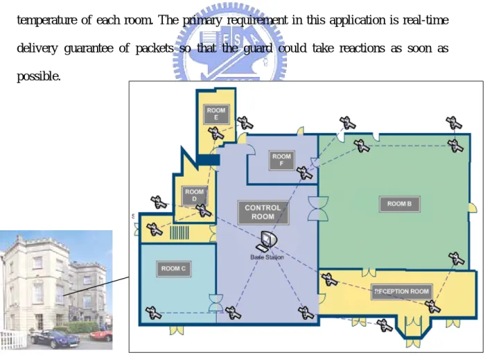
(24) packets which are generated by the sensor nodes that are responsible for the fire as soon as possible. Thus, the applications are latency sensitive. A scenario example is a fire detection system used in museum as shown in Figure 3-1. Figure 3-1 (a) shows the appearance of this museum and Figure 3-1 (b) shows the floor plan. The building is divided into several rooms. Each room contains one or more sensor nodes. There are also some sensor nodes outside the building to detect the temperature around the museum. In the control room, a base station is set up to receive wireless packets. In Figure 3-1 (b), the satellite-like objects denote the sensor nodes. And the dotted lines denote the relay paths which data propagate along. These sensor nodes detect the temperature in their spot by using thermistor sensor and relay this information to base station. Base station provides guard the information about the temperature of each room. The primary requirement in this application is real-time delivery guarantee of packets so that the guard could take reactions as soon as possible.. Figure 3-1： Scenario Example - Fire Detection System. 17.

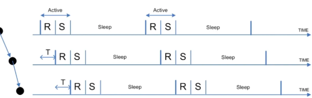
(25) These assumptions about the network and application affect the proposed LAMAC protocol design strongly. It also motivates the differences of LAMAC from the existing protocol such as S-MAC.. 3.2. Basic Scheme. The major cause of transmission latency in S-MAC is the sleeping latency. When a sensor node gets a packet to send, it must wait until its receiver wake up. In the design of S-MAC, each frame is much larger than the active slot. If a node gets a packet right after the active slot, it must wait almost the whole frame time to transmit this packet. Even in an average case, it still needs to wait halt of the frame. The larger the frame, the longer the latency. If the intended receiver can wake up just at the moment that some other node wants to send packets to it, the sleeping latency will be eliminated. This is the main idea of LAMAC. We use a stair-like scheduling MAC protocol to achieve this goal.. Figure 3-2： Data forwarding path and Stair-like Wake-up schedule. Figure 3-2 shows a data forwarding path and its stair-like wake-up schedule. We use the similar frame structure with S-MAC. Each frame is divided into two periods. 18.

(26) One is active period which is also called the duty cycle and the other is sleeping period. The difference between our frame from S-MAC is that the active period is further divided into two slots, the receiving slot and the sending slot. In Figure 3-2, the R slot denotes the receiving slot. And the S slot denotes the sending slot. In sending slot, nodes contend for the communication medium. Then the winners send their packets to their next hop nodes. In receiving slot, nodes wait for neighbors to send packets to them. In sleeping period, nodes turn off their radio to save energy. The sending slot and receiving slot both have length of T. This length is long enough for nodes to contend for the medium and transmit one packet. Along the data forwarding path, an offset of T is used to schedule the wake-up time. Each receiver on the path wakes up T interval later than its sender. This means that each receiver will wake up just at the moment that its sender enters the sending slot. The advantage of this schedule is that once a node receives a packet from another node, it can immediately enter the sending slot and transmit this packet to next hop node. According to our assumptions about network data flow, every data packet in the network has a forwarding direction toward base station. Base station acts as a collector to gather all data packets in the network. Because base station is the root of the data gathering tree, every routing path ends in base station. This topology gives us a convenience to arrange the wake-up schedule of the whole network. Every node has an offset length T of wake-up time according to its hop count away from base station. Because of the infinite power, base station is always at receiving state without sleeping. So the wake-up time of the nodes which are one hop away from base station does not have offset. In our schedule design, these nodes wake up for the first time when the system start. Their schedule is called the base schedule. The nodes which are two hops away from base station have an offset T to the system starting time. And the nodes which are three hops away have an offset 2T. More generally, the node 19.

(27) which is k hops away from base station has an offset (k-1)T of wake-up time to the system starting time.. 3.2.1 Contention Mechanism In wireless sensor networks, if more than one neighbor node wants to transmit packet, they need to contend for the transmission medium to avoid collision. Among contention based protocols, S-MAC does a good job in designing the contention mechanism. We use the similar mechanism with SMAC. The contention mechanism uses a Request-To-Send（RTS）, Clear-To-Send（CTS）, Acknowledgement（ACK） scheme, which provides both collision avoidance and reliable transmission. Before transmitting a packet, physical carrier sense is performed at the physical layer by listening to the medium for possible transmissions of other packets. For example, if a sensor node wants to send a packet, it starts carrier sense when it enters the send slot. It randomly selects a time slot within a fixed contention window to finish its carrier sense. By the end of the random time, if the node has not sensed any transmission, it wins the medium and starts sending its RTS packet to the receiver. But if the node senses another transmission before the random time slot ends, it considers itself to lose the medium. The node then goes to sleep and wakes up at the next active period. Another losing case is when a sensor node sends RTS packet but fails to receive CTS packet. This means there is a node which is outside its communication range but has the same intended receiver with it wins the contention.. 20.

(28) Figure 3-3： An example of contention process. An example is shown in Figure 3-3, node B and C both want to send packets to node A at the same time. Node B and C are in the same collision domain. They first generate a random carrier sense time which is denoted by CS in the figure to perform carrier sense. Because of the shorter CS time, node B is able to send the RTS packet to node A by the end of the CS. As long as node C senses the RTS packet from node B, it considers itself to lose the medium. Node C then ends carrier sense and goes to sleep. After receiving the CTS packet, node B starts the data packet transmission. In addition to collision avoidance problem in the same collision domain, the hidden node problem is well known in wireless and ad hoc networks. This is what we mentioned above about a node outside some other node’s communication range but has the same receiver with it. The RTS-CTS scheme is sufficient to solve this hidden node problem. Although there is a little overhead of using this scheme, the overhead is worthwhile comparing with significant energy used in retransmitting packets.. 21.

(29) Figure 3-4： Structure of Send slot. 3.2.2 The structure and length of active period The active period is divided into sending slot and receiving slot. These two slots have the same length. Here we take sending slot as our example. Figure 3-4 shows the structure of sending slot, the sending slot is divided into two intervals. One is contention interval and the other is transmission interval. As mentioned earlier, a node should perform carrier sense before sending a packet. It randomly generates a time slot within a fixed contention window to finish its carrier sense and then send its RTS packet. After sending its RTS packet, the node waits for CTS packet from the receiver. When it gets CTS packet, the contention mechanism finishes. The contention interval must be long enough to contain all these process. This observation gives us a limit on the length of the contention interval： The length of contention interval ＝ W + R + T + C where W is the length of the fixed contention window, R is the length of an RTS packet, T is the turn-around time（the short time between the end of the RTS packet and the beginning of the CTS packet）, and C is the length of an CTS packet. The transmission interval is responsible for data packet transmission. The length of the interval must be long enough to transmit a whole data packet and an acknowledge packet. The contention interval plus the transmission interval is the sending slot. And the receiving slot has the same length with send slot. Thus the active period is twice 22.

(30) the length of the sending slot. In our stair-like wake-up schedule, the offset T is exactly the length of the sending slot.. 3.2.3 Maintaining Synchronization Since LAMAC is contention-based protocol, neighboring nodes which are in the same hop count must synchronize to contend the communication medium. The clock drift on each node can cause synchronization errors. Two techniques are used to make it robust to such errors. First, the active period is significantly longer than clock drift. Some experiments have shown that the clock drift between two nodes does not exceed 0.0002 s per second. Mostly the active period is more than 104 times longer than the clock drift rates. Compared to TDMA schemes with very short time slots, LAMAC requires much looser time synchronization. Second, all exchanged timestamps are relative rather than absolute. Although the long active time can tolerate clock drift, neighboring nodes still need to periodically update their schedules with each other to prevent long-term clock drift. The synchronization scheme we used is similar to S-MAC. As described in the related work chapter, schedule synchronization in S-MAC is accomplished by sending a SYNC packet. The SYNC packet is very short, and includes the address of the sender and the time of its next sleep. The next sleep time is relative to the moment that the sender starts transmitting the SYNC packet. When a receiver gets the SYNC packet, it adjusts its timer according to the value in SYNC packet. We have modified this scheme to fit the proposed protocol. Instead of sending SYNC packets, we use the CTS packet to do the same thing. Each CTS packet contains a field to indicate the time of its next sleep. The time is also relative rather than absolute. We can reduce the. 23.

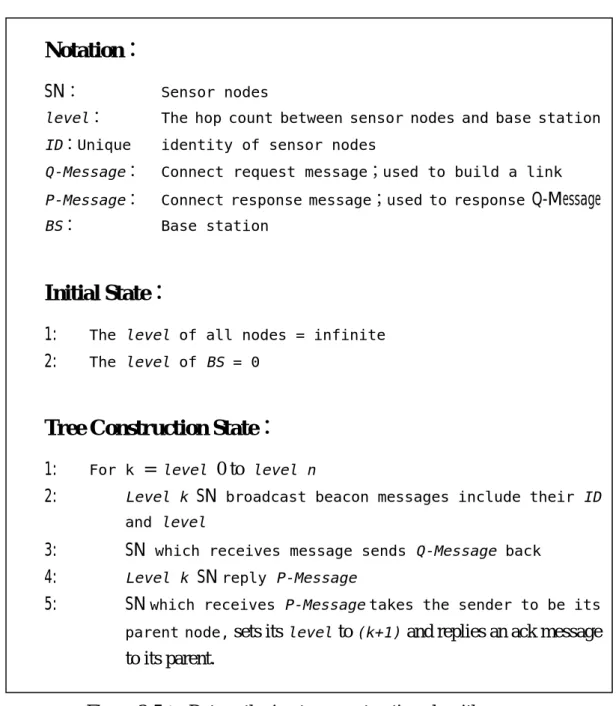
(31) SYNC period in S-MAC without using SYNC packet. This makes LAMAC more energy efficient.. 3.2.4 Scheme of data gathering tree construction In the proposed LAMAC protocol, every node has a specific wake-up schedule according to its hop count from base station. Thus we need some information to recognize the position of all nodes in their routing path. Sensor nodes can adjust their wake-up schedule to the position. It means we need to construct data gathering tree of the whole network to locate sensor nodes. There are some data gathering tree construction schemes mentioned in Chapter I. We use the similar scheme with” NeuRFon Netform ” which is presented by L. Hester and Y. Huang. They construct data gathering tree according to the hop count of each node. In the beginning of construction period, every node listens for beacon packets. The first node to start the construction, the base station, begins to broadcast beacon packets. These packets contain two fields. One is ID field which indicates the sender’s ID, and the other is depth field which indicates the hop count of the sender from base station. The nodes which are able to receive these beacon packets form base station are within the communication range of base station. They can communicate with base station without intermediate nodes. After receiving the beacon packets, the nodes send connection request packets to base station. These packets contain the sender’s ID and are used to request the base station to be its parent node. Base station will reply connection response packets to these nodes to accept the requests. Each node which has received reply takes base station to be its parent and sets its level to 1. All of the 24.

(32) nodes which are one hop away from base station form the level-1 nodes. Then these level-1 nodes broadcast their own beacon packets include their ID and level. In our data gathering tree, the level of a node means its hop count from base station. The same procedures are performed between level-1 nodes and those nodes which are able to receive beacon packets. After the procedures finish, these nodes will from level-2 nodes. The construction procedure repeats until all sensor nodes have their own level and parent. The detailed description of the construction scheme is shown in Figure 3-5. In the data gathering tree, the level-1 nodes are those which are within the communication range of base station. And level-2 nodes are those which are within the communication range of level-1 nodes but are outside of the range of base station. More generally, level-m nodes are those which are within communication range of level-(m-1) nodes, but are outside the range of base station, the level-1 nodes, the level-2 nodes, …, and the level-(m-2) nodes. Every node, with the exception of base station, has a single parent node, which is a node within its communication range and is one level higher than this node. Each sensor nodes will keep a list which is called “upper layer list”. This list indicates the nodes which are one level higher and can be accessed by the owner of this list. Sensor nodes will construct this list during tree construction period. For example： After level-k nodes finish their construction procedure, level-k nodes will broadcast their own beacon messages which contain their ID and level to construct level-(k+1) nodes. Sensor nodes which receive the beacon messages from level-k nodes will be the level-(k+1) nodes. When sensor nodes receive these beacon messages, they will add the owners of beacon messages into their “upper layer list”. After the level-(k+1) nodes construction procedure finishing, each level-(k+1) nodes will also complete the “upper layer list” construction. 25.

(33) Notation： SN：. Sensor nodes. level：. The hop count between sensor nodes and base station. ID：Unique. identity of sensor nodes. Q-Message：. Connect request message；used to build a link. P-Message：. Connect response message；used to response Q-Message. BS：. Base station. Initial State： 1: 2:. The level of all nodes = infinite The level of BS = 0. Tree Construction State： 1: 2:. For k = level 0 to level n Level k SN broadcast beacon messages include their ID and level. 3: 4: 5:. SN which receives message sends Q-Message back Level k SN reply P-Message SN which receives P-Message takes the sender to be its parent node, sets its level to (k+1) and replies an ack message. to its parent. Figure 3-5： Data gathering tree construction algorithm. When the data gathering tree construction process completed, each sensor nodes can arrange its own wake-up schedule according to its level on the routing path. However, some links between sensor nodes may be broken due to the unreliable feature of wireless sensor networks. Harsh environment is one source of unreliability. Besides this, sensor nodes may fail due to some reason such as energy exhaustion. These unreliable features may cause the data gathering tree to lose its connectivity. Thus, the data gathering tree needs to be reconstructed every a specific interval. 26.

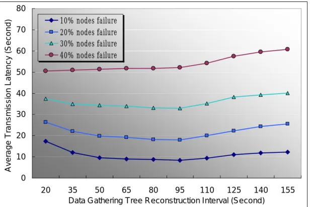
(34) However, data gathering tree reconstruction may cause some overhead such as energy and transmission latency. This is because when network is in reconstruction mode, data packets need to be queued in sensor nodes instead of forwarding to the base station. Sensor nodes have to keep waking up to process beacon messages in the whole tree reconstruction period. These overheads have to be reduced as possible. Thus, we simulate the overheads caused by different reconstruction interval. We uses 4 conditions to simulate these overhead. The condition of”10% nodes failure” indicates that every a specific interval, there will be 10% nodes losing their function and can not forward and process any data packets any more. The other conditions are similar. The results are shown in Figure 3-6 and 3-7. As shown in Figure 3-6, when reconstruction interval is short such as 20 seconds or 35 seconds, the advantage of tree reconstruction is not obvious. Especially when node failure rate is 10%, the overhead of transmission latency caused by short reconstruction interval becomes too serious to be accepted. As the result shows, the interval of 95 seconds may be an acceptable interval. Figure 3-7 shows the overhead of energy consumption. The similar conclusion of 95 seconds interval is also made. Thus, we will reconstruction our data gathering tree every 95 seconds.. 27.

(35) Average Transmission Latency (Second). 80 10% 20% 30% 40%. 70 60. nodes failure nodes failure nodes failure nodes failure. 50 40 30 20 10 0 20. 35 50 65 80 95 110 125 140 Data Gathering Tree Reconstruction Interval (Second). 155. Figure 3-6： The overhead of transmission latency caused by reconstruction. Energy Consumption per Packet (mJ). 50 10% nodes failure 20% nodes failure. 45. 30% nodes failure 40% nodes failure. 40 35 30 25 20 20. 35 50 65 80 95 110 125 140 Data Gathering Tree Reconstruction Interval (Second). 155. Figure 3-7： The overhead of energy caused by reconstruction. However, some applications require critical real-time data transmission. The 95. 28.

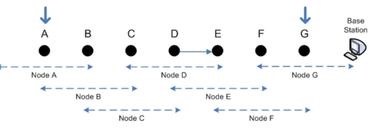
(36) seconds interval is still too long for these applications. Thus, we introduce a temporal path mechanism to adapt these applications. Take advantage of the “upper layer list”, each sensor node is able to know which one level higher node can be accessed by it. By temporal path mechanism, sensor node will regard its parent node to be failure when it fails to receive the ACK message three times. As long as a sensor node regards its parent node to be failure, it will randomly choose one node from its “upper layer list” to be its temporal parent and transmit data packets to this temporal parent until next data gathering tree reconstruction. This mechanism can help nodes to reconstruct their paths between each tree reconstruction. However, this mechanism can not find the best parent node for each sensor node. Thus, the data gathering tree reconstruction is still needed because it can build the better data gathering tree.. 3.2.5 Overhearing Avoidance In most wireless networks, wireless devices always keep radio on to listen to all data transmissions. In 802.11 CSMA, this overhearing is used to perform effective virtual carrier sense. As a result, each node overhears many packets which are not assigned to it. This causes a significant energy waste, especially in dense and heavy traffic networks. Figure 3-8 shows a multi-hop network which is formed by seven sensor nodes and a base station. The data flow in this network is from node A to base station. Each node can only hear the transmission from its immediate neighbors. For example, node D can hear the transmission form node C and E. But node D can not hear the transmission from node F to E or B to C. The dotted lines denote the interference areas of each sensor nodes. Suppose node D is currently transmitting a data packet to 29.

(37) E. The CTS packet from node E would be heard by node F and the RTS packet from node D would be heard by node C. Thus node F should go to sleep since its transmission interferes with E’s reception. Node C should also go to sleep because its reception would be interfered by node D’s transmission. This means node B can not transmit any packet to node C. In the network, only node A and node G can still work now. This illustrates a conclusion that if a node is in transmission, the nearest nodes able to transmit must be at least three hops away. The sensor nodes which are one or two hops away should go to sleep to save energy. This is a quite important conclusion that affects the design of LAMAC.. Figure 3-8： A multi-hop network and interference range of each node. 3.2 Adaptive Sleeping The scheme of periodically listen and sleep is able to reduce the energy and time spent greatly on idle listening. However, when a sensed packet generated, it is desirable that the sensed data can be transmitted through the network without too much delay. When each node strictly follows its active-sleep schedule, there is a potential delay on each hop. And the average value is proportional to the length of the 30.

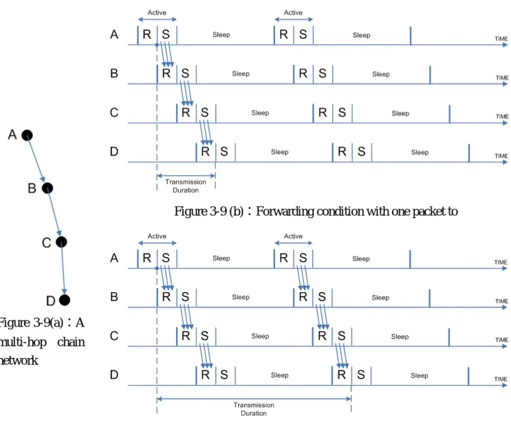
(38) frame. We therefore introduce a technique called adaptive sleeping to reduce transmission latency and use active-sleep cycle more flexible and efficiently.. 3.3.1 The latency of multiple data forwarding As long as MAC protocol use sleep-active cycle schedule, the sleeping latency will happen. For example, the most critical latency in S-MAC is the sleeping latency. Sleeping latency is the most serious delay among all kinds of transmission latency. And it also exists in LAMAC. We use an example to illustrate the sleeping latency in our proposed protocol. Figure 3-9(a) shows a multi-hop chain network. In this network, data flow is from node A to node D. Figure 3-9(b) and 3-9(c) show the time relationship and packet forwarding condition among all sensor nodes. As shown in Figure 3-9(b), only one packet is transmitted through the network. Because of the stair-like schedule, this packet goes through the network without sleeping latency. The transmission duration of this packet is shown in below of Figure 3-9(b). This is an ideal case and only happens in networks whose traffic is very light. Figure 3-9(c) shows a network with average traffic. Node A gets two packets to transmit. The first packet is transmitted without sleep latency. But node A is not able to transmit the second packet until next sending slot. This is because one sending slot is only long enough to transmit one packet. The whole transmission duration is shown in Figure 3-9(c) below. This duration is much longer than that of Figure 3-9(b) because of the sleep period. As long as a node has more than one packet to transmit, it needs many sending slots to handle all packets. Once a node waits for another sending slot, sleeping latency happens. The sleeping latency will significantly reduce throughput and increase the overall transmission latency. We therefore introduce a mechanism to 31.

(39) switch the nodes from the low-active-cycle mode to a more active mode in this case.. Figure 3-9 (b)：Forwarding condition with one packet to. Figure 3-9(a)：A multi-hop chain network. Figure 3-9 (c)：Forwarding condition with two packet to Figure 3-9： An example of sleeping latency. 3.3.2 Adaptive Sleeping Scheme We propose an important technique, called adaptive sleeping, to reduce the transmission latency caused by the periodic sleep of each node in a multi-hop network. The basic idea is to let receiver know that there are some packets for it but remaining 32.

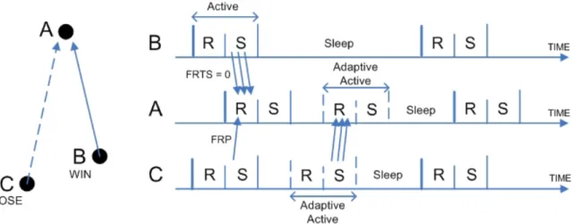
(40) active time is not long enough to transmit these packets. It works as follows： if a node gets more than one packet to transmit, it will set the future-request-to-send （FRTS） flag of these packets except the last packet. The receiver will hold another extra active period during sleep period for these packets. We call the extra active period ”adaptive active period”. Figure 3-10 shows an example of adaptive sleeping. Node A has two packets to transmit to node B. In the original active period, node A transmits the first packet to node B. The FRTS flag of the first packet is set. Node B knows node A has more packets for itself by the FRTS flag. Thus node B holds an adaptive active period which is indicated by dotted line. Node A will use the adaptive active period to transmit the second packet. Having no other packets to send, node A clears the FRTS flag in the second packet. After transmitting the second packet, node A and B both go to sleep until next original active period. If there are more packets to send, node A can set the FRTS flag again. And node B will hold another adaptive active period for these packets. The advantage of using adaptive sleeping technique is that the active-sleep cycle can be used more flexible and be adaptive to different traffic load. Without using adaptive sleeping, sensor nodes need to wait until the beginning of next fame to transmit the second packet. This sleeping latency greatly increases the overall transmission latency and decreases throughput of the whole system. However, by using adaptive sleeping, sensor nodes can switch the low-duty-cycle mode to a more active mode if necessary. This capability can not only reduce transmission latency but also make LAMAC more adaptive to different traffic load.. 33.

(41) Figure 3-10： An example of adaptive sleeping. As mentioned earlier, a node which is currently transmitting packets, the nearest nodes which are able to work must be at least three hops away. This is because the transmissions of packets that are one or two hops away interfere with the current transmission. In Figure 3-11, if node B decides to hold an adaptive active period, it must wait S interval for the current packet to transmit to nodes D which is three hops away from node A. The timing diagram is shown in Figure 3-11. In order to simplify the diagram, only sending slots remain in the figure. There is time slot axis in Figure 3-11 below. We use a sending slot to be one unit of time. In time slot 2, node A transmits a packet to node B. According to our stair-like active schedule, this packet is transmitted to node C in time slot 3 and to node D in time slot 4. Node D is three hops away from node A, the transmission between node D and E will not interfere with the transmission between node A and B. Thus node B can hold an adaptive active period in time slot 5 and receive the second packet from node A. It means if a node wants to hold an adaptive active period, it must wait an S interval of two sending slots to avoid the collision. We let nodes go to sleep to save energy between original active period end and adaptive active period start.. 34.

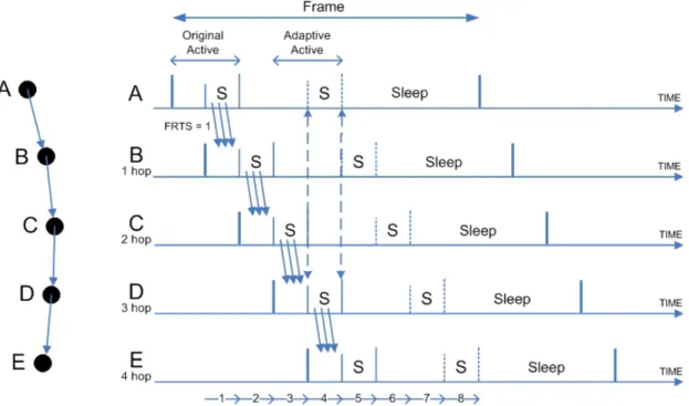
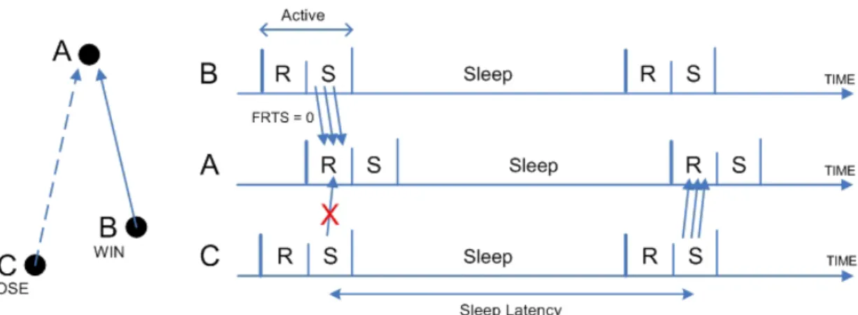
(42) Figure 3-11： Time relationship between two active periods. Once the FRTS flag is set, this flag will not be clear by any nodes. This means every node which receives this packet will hold an adaptive active period. Figure 3-11 shows the mechanism. Node A set the FRTS flag of the first packet. And then this packet will be transmitted through the chain network. Every node will hold an adaptive active period after two sending slot. This makes the second packet transmitted through the path without sleeping latency. But even we use the adaptive sleeping technique, sleeping latency still happens in some special cases. Figure 3-12 shows an example. Both node B and node C have packet to transmit to node A at the same time. Node B wins the communication medium and transmits its packet to node A. Because of having only one packet to transmit, node B doesn’t set the FRTS flag of its packet. Thus node A will not hold an adaptive active period for further packets. Node C must wait until next send slot to transmit its packet and suffer sleep latency. It is impossible for node B to set the FRTS flag for other sensor nodes because node B never knows whether or not other 35.

(43) nodes have packets to send. Therefore, we introduce a mechanism to enhance the adaptive sleeping technique for this case.. Figure 3-12： Sleeping Latency caused by contention mechanism. We propose a mechanism, called future request-to-send packet (FRP), to reduce the latency caused by contention mechanism. The basic idea is to let receiver know that we still have packets for it, but are ourselves prohibited from using the medium. In this way, if a node loses the communication medium in contention, it will immediately send a future-request-to-send (FRP) packet to its receiver. The FRP packet is very small and only contains the receiver’s ID. Sender’s ID is unnecessary because this packet is used for receiver to hold an adaptive active period. Figure 3-13 shows a similar example to Figure 3-12. Node B and node C contend for the medium and node B wins the contention. As long as node C knows itself loses the medium, it immediately sends a FRP packet to node A. After receiving this FRP packet, node A knows that there are other packets for it. Thus node A will hold an adaptive active period after S interval. The adaptive active period is indicated by dotted line in Figure 3-13. Then node C can use the extra active period to transmit its packet. This mechanism is similar to the function of FRTS flag. By using this mechanism, the. 36.

(44) sleep latency will significantly be reduced.. Figure 3-13： An example of FRP mechanism. Once a node receives the FRP packet, it must pass this packet to next hop node. By this way, the extra active period will propagate along the forwarding path. In addition to reducing sleep latency, the throughput of the network will increase. For the FRP solution to work, the length of active period must be increased slightly. Since the FRP packet is quite small, the increasing value is also small. Compared with the improvement of the throughput and latency, we believe it is worthwhile to use this mechanism.. 37.

(45) 4.. Latency Analysis. When a packet transmits through a multi-hop chain network, it will suffer many difference kinds of delay. The total delay which a packet encounters is called the transmission latency. We will analyze the transmission latency in the following section. The latency in both LAMAC and S-MAC will be analyzed together. And the performance will be compared in the section. When a packet transmits through a multi-hop network, it will encounter the following delays： Contention Delay：Contention delay happens when the sender performs carrier sense. After carrier sensing, the interval for sender and receiver to exchange control packet such as RTS, CTS is included in the contention delay. In some MAC protocols, sender will stay in idle mode when senses some other transmission. This is named back-off delay and is also included in the contention delay. Basically, the contention delay is determined by the contention window size and control packet exchanging interval. Transmission Delay： The transmission delay is the time between the start and the end of a transmission. The transmission delay is determined by the channel bandwidth and packet length. When the packet length increases, the transmission delay also increases. Propagation Delay： The propagation delay is determined by the distance between the sender and receiver. When the distance between the two nodes is quite long, the propagation delay will be a serious problem. However, node distance is normally very small in wireless sensor networks. Thus the propagation delay is often be neglected. Processing Delay： Processing delay refers to the time a node needs to process the. 38.

(46) packet before forwarding it to the next hop. This delay mainly depends on the computing power of the node. In wireless sensor networks, the sensor nodes often do not need to process packets but forward packets to its next hop. Hence the processing delay is quite short. Queuing Delay： Queuing delays happens when the traffic load is heavy. When the traffic becomes heavy, the queuing delay is often the dominant factor of transmission. Sleeping Delay： In order to get good energy efficiency, some MAC protocols introduce the active-sleep schedule to the radio. When a sender gets a packet to transmit, it must wait until its receiver wakes up. The delay is also called sleeping latency and is often determined by the frame length of its active-sleep schedule. We analyze the transmission latency of different MAC protocols in a simple case which the traffic is very light, e.g., only one packet is moving through the network, so that there is no queuing delay. We further assume that the propagation delay and the processing delay can be ignored. We only take contention delay, transmission delay, and sleeping latency into account. Supposed a packet will be transmitted through N hops from source node to base station. By observing the transmission mechanism, we can know that the contention mechanism is immediately followed by the packet transmission. Thus we combine the contention delay and transmission delay to be the CT delay in our analysis and denote its value at hop n by tct,n. Its actual value is determined by different MAC protocol. In LAMAC, its value is equal to the length of sending or receiving period. And in S-MAC, its value is equal to the length of listen slot plus the transmission time of one packet. The value is fixed in both LAMAC and S-MAC because of the fixed length of packets and contention interval. We first look at the MAC protocol without sleeping such as 802.11 CSMA. When a node gets a packet, it immediately starts contention mechanism and tries to forward it 39.

(47) to the next hop. The average delay at hop is tct,n. . The entire latency over N hops is：. Delay ( N ) =. N. ∑ n =1. t ct ,n. (1). Because the length of CT delay is the same at each hop, by change tct,n to the fixed values Tct, we can summarize the value to：. Delay ( N ) = NTCT. (2). Equation (2) shows the transmission latency will increase linearly with the length of hops in the MAC protocol without sleeping. Now we look at LAMAC, which introduces a sleeping latency at each hop. The sleeping latency is denoted by ts,n for the nth hop. In order to reflect a very low duty cycle, we set the sending period to ＜＝ 10% length of a frame. And a frame length is denoted by Tf which is assume to be much larger than tct,n. The delay at hop n is：. Dn = t s ,n + t ct ,n. (3). However, if the node is not the source node which generates the packet, it does not have sleeping latency in LANAC. This is because the sending slot follows immediately the receiving slot in LAMAC. Once an intermediate node gets a packet, it can forward this packet to next hop immediately without sleeping latency. Thus if a node is not the source node, its delay equation must change to：. 40.

(48) Dn = t ct ,n. (4). The delay of source node is denoted by D1 and its equation is：. D1 = t s ,1 + t ct ,1. (5). Because a packet can be generated on the source node at any time within a frame, the sleeping latency on the first hop, ts,1, is a random value which lies in （0, Tf）. And its mean value is Tf/2. Combining the delay on the first hop node and other nodes, we can get the overall delay of a packet over N hops network as：. N. Delay ( N ) = D1 + ∑ Dn n=2. N. = t s ,1 + t ct .1 + ∑ t ct ,n n=2. N. (6). = t s ,1 + ∑ t ct ,n n =1. =. 1 T f + NTCT 2. We assume Tf ＝ k Tct. So equation (6) becomes：. Delay ( N ) =. N 1 Tf + Tf K 2. (7). Equation (7) shows that the multi-hop transmission latency linearly increases with the number of hops in LAMAC. The slope of the line is the Tf /k. Compared with (2),. 41.

(49) although we introduce the sleeping schedule into LAMAC, the transmission latency only increase Tf /2 Now we look at the transmission latency in S-MAC. S-MAC can only forward packet one hop in one frame. The delay at hop n is the same as(3). In S-MAC, contention mechanism only starts at the beginning of each frame. After a node gets a packet in a frame, it has to wait until the next-hop node to wake up. This means it must wait to the beginning of the next frame. This indicates：. Tf. = t ct ,n −1 + t s ,n. (8). Substituting ts,n into equation (3), we obtain：. Dn = T f + t ct ,n − t ct ,n −1. (9). There is an exception on the first hop. As mentioned earlier, a packet can be generated at any time. Thus the delay on the first hop is the same as (5) Combining the equation (5) and (9), we can derive the overall transmission latency in S-MAC as： N. Delay ( N ) = D1 + ∑ Dn n=2. = t s ,1 + t ct ,1 + ∑ (T f + t ct ,n − t ct ,n ) N. n=2. = t s ,1 + ( N − 1)T f + t ct , N. 42. (10).

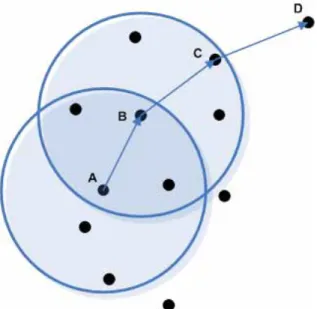
(50) Because that the ts,1 is equal to Tf /2, Tf ＝ k Tct, and tct,N ＝ Tct. Equation (10) becomes. 1 1 Delay ( N ) = NT f − T f + T f 2 K K −2 = NT f − Tf 2K. (11). Equation (11) shows the transmission latency in S-MAC. The slope of the line is the frame length Tf . Because we introduce a very low duty cycle, the value of k is at least 10. Compared the overall latency equation of S-MAC with ours, S-MAC gets much transmission delay according to the sleeping latency. In order to reduce latency，S-MAC uses a technique called adaptive active. The basic idea is to let the node who overhears its neighbor’s transmissions (RTS or CTS) wake up for a short period of time at the end of the transmission. If the node is the next-hop node, its previous hop node is able to pass the data to it immediately instead of waiting for the next frame. If the node does not receive anything during the adaptive listening, it will go back to sleep until its next scheduled listen time. An example is shown in Figure 4-1. In Figure 4-1, node A is currently transmitting a packet to node B. Every node in the transmission range of node A and node B will wake up in the end of the current transmission. The transmission range of node A and B is denoted by the two blue circles in this figure. Node C is in the transmission range of node B and will wake up for the adaptive active. Thus node B is able to transmission the packet to node C when it receives the whole packet from node A. However, the next hop of node C, which is node D, is out of the transmission range of node A and node B. Node D will not perform adaptive active. Hence node C has to wait until the beginning of next hop to transmit this packet to node D. This causes a 43.