針對可調視訊編碼多層編碼控制的快速決策演算法

(1)

國

立

交

通

大

學

資訊科學與工程研究所

碩

士

論

文

針對可調視訊編碼多層編碼控制的

快速決策演算法

A Fast Mode Decision Algorithm for SVC Multi-Layer

Encoder Control

研究生：林哲永

指導教授：彭文孝教授

(2)

針對可調視訊編碼多層編碼控制的快速決策演算法

A Fast Mode Decision Algorithm for SVC Multi-Layer Encoder Control

研究生：林哲永 Student：Jhe-Yong Lin

指導教授：彭文孝 Advisor：Wen-Hsiao Peng

國立交通大學

資訊科學與工程研究所

碩士論文

A Thesis

Submitted to Institute of Computer Science and Engineering College of Computer Science

National Chiao Tung University in partial Fulfillment of the Requirements

for the Degree of Master

in

Computer Science

June 2008

Hsinchu, Taiwan, Republic of China

(3)

針對可調視訊編碼多層編碼控制的快速決策演算法

研究生：林哲永指導教授：彭文孝

國立交通大學資訊科學與工程研究所碩士班

摘

要

基於可調視訊編碼 ( S V C ) 之架構，本論文闡釋一個在使用多層編碼控制下，進行編碼速度優化的問題。傳統由下往上的編碼控制在相對於單層編碼上會有不對稱的編碼效率損失。因此為了能夠在基層和增進層之間的編碼效率上做權衡，多層編碼控制技術已在先前被提出來。然而在現今的方法上，有兩個主要的問題存在 :( 1) 基層使用權重式的 Lagrangian 成本決策方法。(2)增進層則是使用單層編碼決策方法。前者在解決限制式最佳化問題上，其目標函數和限制條件兩者都將會隨著權重因子的選擇而有所變化。此外又因為後者方法不一致的影響，導致了在增進層上發生了無法預期的結果。為了解決這些問題，我們重提了多層編碼控制的公式化問題。並且因為多層編碼控制存在著編碼速度過於緩慢的缺陷，本文利用主導性配對的觀念以及對增進層決策的重新審視，提出了一個兩階段式的快速決策演算法。實驗結果顯示，本文提出的快速決策演算法跟徹底式搜尋所需的 56 組配對相比，我們平均僅需要測試 13 組即可，在這樣的決策組數降低下，編碼平均速度不僅超越徹底式搜尋逾 8 4% ，更在編碼品質上沒有太多的失真。此外，產生出來的實驗結果也顯示，新的快速決策演算法相較於過去的決策演算法上，本方法在給予不同的權重因子中更具有可預測性以及連貫性。

(4)

A Fast Mode Decision Algorithm for SVC

Multi-Layer Encoder Control

Student : Jhe-Yong Lin Advisor : Wen-Hsiao Peng

Institute of Computer Science and Engineering

National Chiao Tung University

ABSTRACT

This thesis addresses the problem of performing fast mode decision for SVC multi-loop encoder control. The conventional bottom-up encoder control is characterized by its uneven distribution of rate-distortion loss relative to single-layer coding. For a tradeoff between the coding efficiency of the base layer (BL) and the enhancement layer (EL), a multi-layer encoder control was proposed. The current approach, however, poses two major problems: (1) it uses the weighted Lagrangian cost as the search criterion for mode decision at the BL and (2) it adopts the single-layer decision criterion for the EL. The former amounts to solving a constrained optimization problem in which both the objective function and the constraints may vary with the choice of the weighting factor, while the latter can sometimes lead to unpredictable results at the EL. To solve these problems, we have revisited the problem formulation of multi-layer encoder control, and have proposed an improved two-stage algorithm by using the concept of dominant mode pairs and by revising the mode decision criterion at the EL. Experimental results show that our fast mode decision algorithm, on average, needs to check only 13 mode pairs, compared to 56 required for the exhaustive search. The mode set reduction leads to a considerable time saving of 84-88%, with an ignorable change in R-D performance. Besides, the results produced with the new decision criterion are more predictable and consistent with different choices of the weighting factor.

(5)

誌

謝

首先我要感謝我的指導教授—彭文孝博士，以及邵家健老師，經由兩位老師一次次給予我在學問研究上的精闢指導，讓這篇論文得以漸趨完整。彭老師凡事追求卓越的精神，對於研究問題深入剖析的嚴謹態度，以及細心與耐心的指導方式，讓我在這兩年的研究生涯中受益良多。在此謹向我的老師致上無限的敬意。其次，這篇論文可以完成，也要感謝交大這個大環境，我要感謝林鴻志學長以及黃雪婷學姐，兩位學長姐在我的研究上擔任了啟蒙的指導，不僅在 H.264 和 SVC 上的專業領域，不辭辛勞的與我討論，更在一開始的研究實作上給予許多珍貴的意見，並且能適時從旁給予建議修正我已偏差的研究方向，使我在這兩年的碩士生涯，不再舉步維艱。謹此對兩人致上由衷的謝意。有榮幸進入 MAPL 實驗室，能夠有熱心與親切的實驗室成員們的切磋與討論，是我在碩士時期最充實的時光。我要感謝其餘的學長姐們—陳渏紋博士、李志鴻博士、林岳進、與陳敏正，一步步帶領我進入這個專業的領域；感謝我的好同學們陳俊吉、詹家欣、與陳建穎，不論是研究上或是生活上，他們總是給予我最直接的協助以及苦樂分享；感謝我的學弟蔡閏旭、王澤瑋、吳崇豪、楊復堯、吳思賢、陳孟傑、黃嘉彥、與李宗霖，在論文撰寫和實驗數據整理方面上，幫了我很大的忙，其中我最要感謝的是蔡閏旭學弟，在最後這一年內，給予了許多無私的協助。最後，我要感謝我的父母—鍾春香女士、林達廣先生的栽培，在爭取碩士學位的路上，給予百分之百的經濟支持與精神支柱，讓我無後顧之憂，能夠專心的在研究領域上打拼。感謝我的妹妹—林瑋芸，給予我滿滿手足的關懷。感謝我的女友—王筱琳，這幾年來辛苦地陪伴、體諒與關心，讓我在孤獨的研究之路上的最低潮時，還能夠感受到一絲溫暖。感謝你們一路的陪伴打氣與支持，在此僅將這篇論文獻給各位，謝謝你們，you are my angles!

(6)

List of Tables

3.1 Test mode space . . . 19

3.2 Test video sequences . . . 19

3.3 The MLEC classes . . . 20

3.4 The EL dominant mode for each class . . . 20

3.5 The comparison results of dominant mode pairs in SOCCER sequence . 23 3.6 The candidate mode pairs for the EL refinement process. . . 26

3.7 The number of checked mode pairs in average. . . 28

4.1 Candidate mode pairs of Schwarz’s fast scheme . . . 32

4.2 RD comparison of Schwarz’s MLEC in soccer sequence . . . 32

4.3 Experimental results of the proposed fast mode decision algorithm with the exhaustive mode decision approach on the QCIF test sequences . . 42

4.4 Experimental results of the proposed fast mode decision algorithm with the exhaustive mode decision approach on the QCIF test sequences (con.) 43 4.5 Experimental results of the proposed fast mode decision algorithm with the exhaustive mode decision approach on the CIF test sequences . . . 43

4.6 Experimental results of the proposed fast mode decision algorithm with

(9)

LIST OF TABLES

the exhaustive mode decision approach on the QCIF test sequences (on

average) . . . 44

the exhaustive mode decision approach on the CIF test sequences (on

average) . . . 45

4.9 The time comparison between proposed MLEC with bottom up encoder

(10)

List of Figures

1.1 The definition of ML-MB pair. . . 2

2.1 Multilayer structure with inter-layer prediction for spatial and temporal scalable coding. . . 6

2.2 The flowchart of inter-layer prediction mechanism. . . 7

3.1 MCM distribution of each class in SOCCER sequence. . . 21

3.2 The analysis of combined mode pair distribution. . . 23

3.3 Cross-layer mode pair distribution in diﬀerent weighting cases in SOC-CER sequence. . . 25

3.4 The flowchart of the proposed fast mode decision algorithm. . . 27

4.1 The RD curves of Schwarz’s MLEC with fixed QP setting. . . 33

4.2 The RD curves of the higher weighting cases. . . 33

4.3 The analysis of the alteration degrees in the Schwarz’s MLEC. . . 35

4.4 The RD curves of proposed MLEC with fixed QP setting. . . 37

4.5 The analysis of the alteration degrees in the proposed MLEC. . . 38

4.6 Adjustment for the Lagrange multiplier with iteratively selecting QP. . 40

4.7 RD comparison between proposed MLEC and Thomas’s MLEC with iteratively selecting QP . . . 41

(11)

LIST OF FIGURES

4.8 The RD curves of QCIF sequences. . . 46

(12)

CHAPTER 1 Introduction

1.1 Background

Considering the diﬀerent devices with varying capabilities and the heterogeneous net-works used to deliver video contents, scalability becomes a desirable feature in many video applications. For this reason, the Joint Video Team (JVT) has recently, based upon H.264/AVC, standardized a scalable video coding standard [1] (referred hereafter as SVC).

The SVC supports spatial, temporal, SNR and their combined scalability within a single bitstream, which can be extracted and partially decoded to provide lower spatiotemporal resolutions or reduced quality. The spatial and quality scalability are achieved via a layered coding approach, while the temporal scalability is based on using hierarchical temporal prediction, which is already supported by the syntax of H.264/AVC. Because the layered coding introduces a high degree of redundancy into coding layers, the SVC additionally provides an adaptive inter-layer prediction mech-anism to reuse as much lower layer information as possible.

(13)

Sec 1.2. Problem Statement

I

P

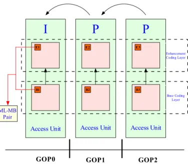
ML-MB Pair

Access Unit Access Unit Access Unit

B1 B2 B3 E3 E2 E1 Enhancement Coding Layer Base Coding Layer

GOP0 GOP1 GOP2

♦((B1,E1), (B2,E2), (B3,E3) are co-located MBs

Figure 1.1: The definition of ML-MB pair.

layer (EL), the Joint Scalable Video Model (JSVM) [2] adopts a bottom-up encoder control (BUEC), with which the coding parameters of the BL are first determined without regard to the content of the higher ELs and then based on these data, the higher ELs are coded sequentially. The BUEC is characterized by its uneven distribution of rate-distortion (R-D) loss relative to single-layer coding: the higher layers usually suﬀer from more coding eﬃciency losses than the lower layers. This is due to the sequential manner in which the mode decision is carried out.

1.2 Problem Statement

For a tradeoﬀ between the BL and the EL quality, Schwarz et al. [3] proposed a multi-loop encoder control (MLEC), which weights the Lagrangian cost of the BL against that of the EL during the mode decision. As shown in Figure 1.1, the basic unit for mode decision in MLEC is composed of a pair of MBs: one from the BL and the other one from the corresponding MB at the EL. For each ML-MB pair, its mode space is the cartesian product of the BL and the EL mode sets, i.e., all possible ordered pairs of the BL and the EL coding modes. In view of the huge size of the mode space, a fast mode decision algorithm is thus desirable and advisable for MLEC.

(14)

Chapter 1. Introduction

et al. [3] provided a two-stage mode decision algorithm. In the first stage, each ad-missible BL mode is associated with its most probable EL mode to form a mode pair, and the mode decision for the BL is conducted by comparing the weighted Lagrangian cost. In the second stage, the EL mode is searched exhaustively conditional on the BL mode as in BUEC. With the two-stage process, the computational complexity of MLEC is reduced to a level similar to that of BUEC. However, when viewed from the mode decision criterion, it poses two major problems:

• Using the weighted Lagrangian cost as the search criterion for mode decision amounts to solving a constrained optimization problem in which both the objec-tive function and the constraints may vary with the choice of the weighting factor. However, in the contexts of MLEC, it makes more sense to alter the objective function while leaving the constraints unchanged.

• Adopting the single-layer decision criterion for the EL may fail to attain the optimal solution and can lead to unpredictable results. In some cases, one could even end up with a worse EL performance when the preference is actually given to the EL quality.

To solve these problems, we have revisited the problem formulation of MLEC and have improved the two-stage algorithm in a number of significant ways.

1.3 Contributions

Specifically, our main contributions in this work include the following:

• We have reformulated the problem of MLEC and, based on the problem formu-lation, proposed a new decision criterion.

• We have improved the two-stage algorithm by using the concept of dominant mode pairs and by revising the mode decision criterion at the EL.

• We have conducted a detail analysis on how the mode distributions at the BL and EL may vary with the weighting factors.

• We have compared the performance of our proposed scheme with that of the exhaustive search and that of [3].

Experimental results show that our fast mode decision algorithm, on average, needs to check only 13 mode pairs, compared to 56 required for the exhaustive search. The

(15)

Sec 1.4. Organization

mode set reduction leads to a considerable time saving of 84-88%, with an ignorable change in R-D performance. Besides, the results produced with the new decision criterion are more predictable and consistent with diﬀerent choices of the weighting factor. In the comparison with Schwarz et al.’s approach, which leads to a time saving of 73-74%, the faster encoding speed can be achieved by our proposed algorithm.

1.4 Organization

This thesis is organized as follows: Chapter 2 contains the RDO problem formulation for BUEC and MLEC. Chapter 3 presents the proposed formulation and the fast mode decision criterion. Chapter 4 presents the similation results and compares the pro-posed scheme with the previous work [3]. Finally, Chapter 5 gives a summary of our observations and a list of future works.

(16)

CHAPTER 2 Scalable Video Coding and its Encoder

Control

2.1 Introduction to SVC

2.1.1 Concept

The scalable video coding (SVC) standard is a scalable extension of the H.264/AVC standard developed by the Joint Video Team (JVT). An SVC bitstream is organized into one BL and one or more ELs in corresponding scalable dimensions and a subset of that can be extracted to produce a lower playback quality. SVC supports three types of scalabilities:

1. Spatial scalability: The correlations among diﬀerent spatial resolution layers is exploited by the adaptive inter-layer prediction techniques. (Multiple levels of frame resolution)

2. Temporal scalability: It is provided by hierarchical temporal prediction structures for each coding layer. (Multiple levels of frame rate)

(17)

Sec 2.1. Introduction to SVC

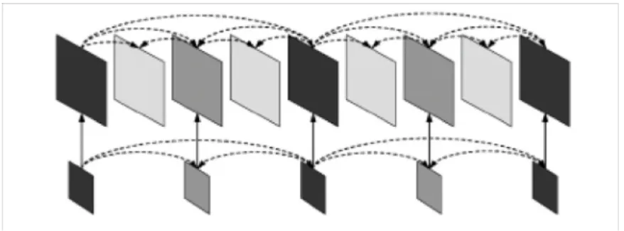
Figure 2.1: Multilayer structure with inter-layer prediction for spatial and temporal

scalable coding.

3. Quality scalability (Multiple levels of quality) in SVC is provided by two ap-proaches:

• Coarse-grain quality scalable coding (CGS), which can be considered as a special case of spatial scalability with identical frame sizes for the BL and the EL.

• Medium-grain quality scalable coding (MGS), which provides quality refine-ment layers inside each spatial layer and allows packet-based quality scalable coding.

SVC follows the conventional approach of multi-layer coding, which is also used in H.262 MPEG-2 Video, H.263, and MPEG-4 Visual. Each layer is referred to by a dependency identifier D. The dependency identifier for the BL is equal to 0, and it is increased by 1 from one spatial layer to the next. In order to improve coding eﬃciency, additional so-called inter-layer prediction mechanisms are incorporated as illustrated in Figure. 2.1. An access unit is formed by the representations with diﬀerent spatial resolutions for a given time instant. As illustrated in Figure. 2.1, lower layer pictures are possible to combine temporal and spatial scalability, because they don’t need to be present in all access units.

2.1.2 Inter-Layer Prediction

For improving rate-distortion eﬃciency of the ELs, the main goal of the development of inter-layer prediction tools is to use as much lower layer information as possible. Usually, for the reason of improvement of the coding eﬃciency for ELs, the inter-layer predictor need to compete with the temporal predictor. Thus, two additional

(18)

inter-Chapter 2. Scalable Video Coding and its Encoder Control

Start

base mode flag

Derive mvp, ref. index from the base layer

Derive mvp, ref. index from the enhancement layer 0

1

Compute the motion information

Compute the residual information

ModeBLis Intra motion prediction_flag

0 1

Derive all motion infomation from the base layer (BLSkip) Inter-layer intra predic tion

(IntraBL)

residual prediction flag

0 1

Inter-layer residual prediction H.264/AVC residual prediction

YES NO

path 1 _{path 2} _{path 3} _{path 4}

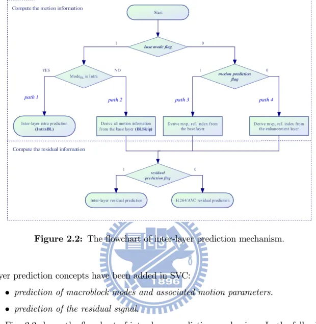
Figure 2.2: The flowchart of inter-layer prediction mechanism.

layer prediction concepts have been added in SVC:

• prediction of macroblock modes and associated motion parameters. • prediction of the residual signal.

Fig. 2.2 shows the flowchart of inter-layer prediction mechanism. In the following subsections, the three inter-layer predictions are introduced by illustrating this figure.

2.1.2.1 Inter-Layer Motion Prediction

When the reference layer MB is inter-coded, the EL MB is also inter-coded. In that case, the partitioning data of the EL MB together with the associated reference indexes and motion vectors are derived from the corresponding data of the co-located MB in the reference layer by so-called inter-layer motion prediction. For inter-layer motion prediction, SVC includes two diﬀerent implementations:

1. BLSkip mode: A new MB type of SVC, it is illustrated in the path 2 of Fig. 2.2, which is signaled by a syntax element called base mode flag. For this MB type, all motion information is derived from BL; thus, only residual signal but no

(19)

Sec 2.2. SVC Encoder Control

additional side information such as inter-prediction modes or motion parameters is transmitted.

2. Inter-layer motion vector prediction: When the base mode flag equals to 0 and the motion prediction flag equals to 1 as shown in the path 3 of Fig. 2.2.

• The motion vector predictors (mvp) of the EL are derived from the motion vectors of the BL.

• The reference indexes of the EL are also derived from the BL.

2.1.2.2 Inter-Layer Intra-Prediction

When base mode flag equals to 1 and the corresponding MB of the reference layer is intra-coded, the current MB is predicted by inter-layer intra-prediction as explained in path 1 of Fig. 2.2, for which the corresponding reconstructed intra-signal of the reference layer is used as the predictor of current MB. In this inter-layer prediction, the current MB type is called IntraBL mode.

2.1.2.3 Inter-Layer Residual Prediction

A flag, called residual prediction flag, is added to the MB syntax for ELs as shown in the bottom of Fig. 2.2, which signals the usage of inter-layer residual prediction. It can be employed for all inter-coded MBs regardless whether they are coded using the newly introduced SVC MB type signaled by the base mode flag or by using any of the conventional MB types. When this residual prediction flag equals to 1, the residual signal of the corresponding MB in the reference layer is used as prediction for the residual signal of the EL MB, so that only the corresponding diﬀerence signal needs to be coded in the EL.

2.2 SVC Encoder Control

The inter-layer prediction of SVC supports single-loop decoding by allowing a single motion compensation loop; a complete reconstruction of lower layer pictures is not required. However, the encoder generally needs to be operated in multi-loop mode in order to avoid drift between encoder and decoder reconstruction for all layers of an SVC bit-stream.

(20)

Chapter 2. Scalable Video Coding and its Encoder Control

The encoder control for SVC specifies a bottom-up process in which first the BL and then the EL is encoded. It leads to an uneven distribution of the coding efficiency losses relative to single-layer H.264/AVC coding between BL and ELs. The bottom-up process is introduced in Section 2.2.1. The R-D optimized MLEC, which makes it possible to trade off BL and EL coding efficiency and to generally improve the effectiveness of fidelity scalable coding, is introduced in Section 2.2.2. Although the r-d optimized MLEC can trade off BL and EL coding efficiency, the encoding time is considerable.

2.2.1 Bottom-up Encoder Control

The JSVM [2] encoder control specifies that the encoder decisions for all layers are made in sequential order starting at the bottom layer. The decision problems can be formulated as the following objective optimization problem for each layer i:

min Di(pi|pi−1...p0)

s.t.

R0(p0) + R1(p1|p0) + ... + Ri(pi|pi−1...p0)≤ Rci

(2.1)

Di and Ri represent distortion and rate for JSVM encoding layer i, respectively. Rci

is the maximum target bit-rate in layer i. For each access unit, at first the coding

pa-rameters p0 for the BL are determined following the widely-used Lagrangian approach

[4],

p0 = arg min

{p0}

D0(p0) + λ0· R0(p0) (2.2)

without considering their impact on the ELs. D0(p0) and R0(p0) respectively

rep-resent distortion and rate associated with selecting parameter vector p0. λ0 is the

Lagrange multiplier, which is determined based on the chosen quantization parameter

QP0. Similarly to the BL, coding parameters pi for each EL i are determined by

min

{pi|pi−1...p0}

Di(pi|pi−1...p0) + λi· Ri(pi|pi−1...p0) (2.3)

given the already determined coding parameters p_i−1 to p0 for the lower layers the

(21)

While the BL coding efficiency is basically identical to that of single-layer coding (minor losses may result from the mandatory usage of constraint intra prediction in SVC), there is usually a loss in coding efficiency for the ELs. Because the chosen BL coding parameters are optimized for the BL only and are not necessarily suitable for efficient EL coding, the effective reuse of the BL data for EL coding is limited. For the reason of trading off coding efficiency between BL and ELs, the solution for this tradeoff problem is detailed in the following sections.

2.2.2 Multi-layer Encoder Control

The explicit bit allocation (EBA), which can trade off motion information and residual information, has been well studied in image and video coding [5]. The feature of EBA is that bits can be shifted among different regions according to their relative importance such that the overall visual quality could be optimized. From this point of view, the R-D performance of the BL and the R-D performance of the EL can be seen as two different regions, and the tradeoff problem between these regions can also be seen as a kind of explicit bit allocation (EBA) problem in SVC. This EBA problem is introduced in Subsection 2.2.2.1, and the reasons of development for our proposed MLEC formula are concluded in the end.

Furthermore, there is a diﬀerent type of bit allocation criterion, called implicit bit allocation (IBA). The feature of IBA is that bits allocated to each region are "fixed" and only "control policy" can be made according to the relative importance of each region. From the point of view to trade oﬀ BL and ELs, the "control policy" can be seen to make the corelations between Langrangian factor λ of each layer by being involved with the weighting factor assigned to each region. Thus, the IBA method, which has been addressed for the SVC, is introduced in Subsection 2.2.2.2.

In the final Section 2.3, the diﬀerent properties between the EBA method and the IBA method are compared and summarized.

2.2.2.1 Explicit Bit Allocation

In order to overcome the disadvantages of the BUEC, an encoder control of EBA for fidelity scalable coding by joint optimization of BL and EL coding parameter selection has been developed in [3]. Without loss of generality, the modifications of the encoder

(22)

control are described for a simple two-layer configuration; but they can be easily gen-eralized for a multi-layer scenario. In the two-layer scenario, all BL decisions are based on the minimization of the weighted cost function:

min

{p0,p1|p0}

(1_{− w) · (D}0(p0) + λ0· R0(p0)) (2.4)

+ w_{· (D}1(p1|p0) + λ1· (R0(p0) + R1(p1|p0)))

The first and second term of Eq. (2.4), which are adopted from BUEC, represent weighted costs for the BL and the EL, respectively. The weighting factor w [0; 1] controls the trade-oﬀ between BL and EL coding eﬃciency. In order to let the R-D performance of w = 0 case can fit the R-D performance of BUEC, the BL decisions are based on the minimization of Eq. (2.4), but the EL decisions are refined later by the minimization of Eq. (2.3). When w is equal to 1, the BL parameters are only optimized for the EL coding without taking the reconstruction quality of the BL into

account. The coding parameters pi can be seen as the current MB type of layer i in

the mode decision process, on the other hand it can also be seen as the current motion vector of layer i in the motion estimation process. The motion estimation process of MLEC is simplified by Schwarz et al. in [3]. With the general concept of Eq. (2.4), the

minimization proceeds over of the Cartesian product space of p0 and p1. The MLEC

problem can then be reverse derived as the following multiple objective optimization problems: min(1_{− w)D}0(p0) + wD1(p1|p0) s.t. (1) (1_{− w) × (R}0(p0))≤ RB (2) (w)_{× (R}0(p0) + R1(p1|p0))≤ RE (2.5)

RBis the maximum target bit-rate of the BL and RE is the maximum target bit-rate

of the EL. The constraint (2) of Eq. (2.5) is unlimited in w = 0 case, but it converges

to RE when w increases to 1. The objective and constraints vary with the choice of the

weighting factor. However, in the contexts of MLEC, it makes more sense to alter the objective function while leaving the constraints unchanged. Thus, these constraints do

(23)

not make sense. It causes that we can’t obtain the expected RD performance of EL in some high weighting cases and may lead to unpredictable results. Hence, this problem formulation of MLEC is a heuristic solution.

For the above reasons, we have reformulated the problem of MLEC and, based on the problem formulation, proposed a new decision criterion. These details are presented in Chapter 3.

2.2.2.2 Implicit Bit Allocation

An implicit bit allocation (IBA) method, as a tradeoff criterion for the coding efficiency between different regions has been proposed for the combined coarse granular scala-bility (CGS) and spatial scalascala-bility [6]. The IBA is formulated as a multiple objective optimization problem for given that a region which is a quality level at a spatial res-olution and a weighting factor input that is determined by customers’ interests. The IBA exhibits a distinguished feature, which allows bits allocation to each region being fixed and only tradeoff between motion and residual information in each region can be properly set such that coding efficiency of each region is guaranteed in order according to the weighting factor.

Normally, different weighting factors can be assigned to different regions according to their different importances. Obviously, a "control policy" is actually a type of "implicit" bits. If a "control policy" is favorable to a region, more "implicit" bits are allocated there with that region’s coding efficiency becoming relatively higher. In this section, the IBA formula derivation process is briefly introduced.

Let a Lagrangian factor λl,i,j ( = 0.85Q2l,i,j) represents the region corresponding

to the lth temporal level, the jth spatial resolution and the ith SNR level, i.e., λl,i,j

corresponds to the target bit rate ˆγl,i,j. Normally, three SNR layers are suﬃcient for

the CGS at a given spatial level, so we assume that the section contains three SNR layers. Due to rate distortion optimization, the tradeoﬀ between motion and residual information in a region is determined by two quantization parameters, one for ME/MC, and the other for the quantization of residual information. When the CGS range at

the jth spatial level is wide, two pairs of Lagrangian multipliers, (λmv

lo (l, j), λl,j,1)

and (λmv

hi (l, j), λl,j,2) are required to generate two motion vector fields (MVF), which

correspond to (QPmv

(24)

one MVF by (λmv_lo (l, j), λl,j,1) is enough at a spatial level j.

Using the Lagrangian optimization method, the implicit solution to the

optimiza-tion problem can be derived. Since the weighting factor of the (i × j)th region is wl,j,i,

the corresponding Langrangian function is

h = 3 X i=1 J X j=1 wl,j,i ³ Dl,j,i(λmvlo (l, 1), λ mv hi (l, 1), ..., λ mv lo (l, J), λ mv hi (l, J), γl,i,j) + ˜λl,j× γl,i,j ´ From equations { ∂h ∂λmv lo (l,1) = 0 ∂h ∂λmv hi (l,1) = 0 γl,i,j = ˆγl,i,j

and the objective map between ˆγl,i,j and λl,j,i, the optimal solution is solved by a

simplified solution of "Divide and Conquer" presented in [6]. The key idea of "Divide and Conquer" is to simplify the process of obtaining the solution to complex problems by ignoring certain correlations among diﬀerent regions. Thus, the author first uses

this idea to compute two auxiliary values λopt_lo (l, j) and λopt_hi(l, j), which function to

determine the value of λmv_lo (l, j) and λmv_hi (l, j) at a spatial level j. After the "Divide

and Conquer" process, the two auxiliary values λopt_lo (l, j) and λopt_hi (l, j) are obtained as

follows: λopt_lo (l, j) = wl,j,1λl,j,1+ wl,j,2λl,j,2+ wl,j,3λl,j,3 wl,j,1+ wl,j,2+ wl,j,3 (2.6) λopt_hi (l, j) = wl,j,2λl,j,2+ wl,j,3λl,j,3 wl,j,2+ wl,j,3 (2.7) The Eq. (2.6) and Eq. (2.7) reveal the qualitative insight brought by the choices of

λopt_lo (l, j) and λopt_hi (l, j) according to weighting factor wl,j,i.The author uses the

philoso-phy of "think globally" to determine the values of λmv

lo (l, j) and λmvhi (l, j).The customer

oriented scalable tradeoﬀ is achieved by applying, in order, the following rules:

• Rule 1: The ROI corresponding to λoptlo (l, φ(l))has the highest priority to

guaran-tee its coding eﬃciency. (φ(l) is the most important spatial layer in the temporal layer l.).

(25)

Sec 2.3. Comparison and Summary

• Rule 2: Subsequently, the ROI that corresponds to λoptlo (l, j) has the second

highest priority to guarantee its coding eﬃciency at the spatial level j.

• Rule 3: Finally, other regions have the lowest priority to guarantee their coding eﬃciency.

The above IBA solution is further adopted to support two cross-layer motion esti-mation/motion compensation (ME/MC) schemes for the CGS and spatial scalability, which are also presented in the remainder of [6]. In this section, the two cross-layer schemes are not discussed. From the previous presentation of IBA, we find that IBA is a method used to fix the target bitrate and modify the Lagrangian multiplier in each coding layer (region). In this way, two things are achieved:

• The tradeoff of coding efficiency between different coding layers.

• The tradeoﬀ of motion information and residual information in one coding layer. But the encoding process of IBA is still the same as Section 2.2.1.

2.3 Comparison and Summary

The comparison of the BUEC properties and the MLEC properties are summarized as follows:

1. In BUEC, the BL coding eﬃciency is basically identical to that of single-layer coding, but there is usually a loss in coding eﬃciency for the ELs.

2. In BUEC, the eﬀective reuse of the BL data for EL coding is limited, because the chosen BL coding parameters are optimized for the BL only and are not necessarily suitable for eﬃcient EL coding.

3. The BUEC process is a frame level encoding process, but the MLEC process is a MB level encoding process.

4. In MLEC, It can trade oﬀ coding eﬃciency for BL and ELs, but it is a complex encoding process.

The comparison of the IBA properties and the EBA properties are summarized as follows:

1. The feature of EBA is that bits can be shifted among diﬀerent regions according to their relative importance such that the overall visual quality could be optimized. 2. The encoding process of EBA is diﬀerent from the bottom-up encoder process

(26)

and it must be a MB level encoding process in our presented EBA case.

3. The feature of IBA is that bits allocated to each region are "fixed" and only "control policy" can be made according to the relative importance of each region. 4. The encoding process of IBA is still the same as the bottom-up encoder process

and it could be a frame level encoding process in our presented IBA case.

By the above summary, we know the different properties of "BUEC vs. MLEC" and "EBA vs. IBA". In the next chapter, we develop a different encoding process for MLEC, which can determine the coding parameters of one ML-MB pair all at once without fixing the target bit-rate of each layer. Additionally, because the tradeoff scenario of Schwarz’s method is not quite straightforward in the multiple constraints of the objective function, we reformulate the objective function based on the EBA criterion, and it is detailed in the next chapter.

(27)

CHAPTER 3 Fast Mode Decision for Multi-layer Encoder

Control

3.1 Proposed Multilayer Encoder Control

Because the objective and constraints in Eq. (2.5) vary with the choice of the weighting factors w, we developed another RDO formula for MLEC. In the two-layer scenario, the proposed MLEC problem is formulated as the following multiple objective optimization problems: min(1_{− w)D}0(p0) + wD1(p1|p0) s.t. (1) R0(p0)≤ RB (2) R0(p0) + R1(p1|p0)≤ RE (3.1)

Di and Rirepresent the distortion and the bit-rate for encoding layer i, respectively.

RB is the maximum target bit-rate in the BL, while RE is the maximum target

bit-rate in the EL. The weighting factor w [0; 1] controls the tradeoﬀ between BL and EL coding eﬃciency. In this equation, the weighting factor w is not involved in the

(28)

Chapter 3. Fast Mode Decision for Multi-layer Encoder Control

bit-rate constrains of the optimization problem, however the tradeoﬀ property between the BL and the ELs is still retained. The MLEC optimization formula can avoid the weighted constraints regardless of the fitness for the R-D performance of JSVM bottom-up process. Thus, the decisions of the BL and the EL are based on the minimization of the modified cost function:

min

{p0,p1|p0}

(1_{− w) · D}0(p0) + λ0· R0(p0) (3.2)

+ w_{· D}1(p1|p0) + λ1· (R0(p0) + R1(p1|p0))

In the minimization process, the mode decisions in the EL don’t need to be refined

by Eq. (2.3). Di(pi) and Ri(pi) represent the distortion and the rate associated with

selecting parameter vector pi, respectively. The coding parameters pi can be seen as

a current MB type of layer i in the mode decision process. Moreover, it can also be seen as a current motion vector of layer i in the motion estimation (ME) process. We

simplified the BL ME process as the following equation by assuming v0 ' v1:

min

{v0,v1|v0}

(1_{− w) · D}0(v0) + w· D1(v0) + (λ0+ λ1)· R0(v0) (3.3)

In this equation, v0 and v1 represent the motion vectors of the BL and the EL,

respectively. The distortion Di(v0) and the bit-rate Ri(v0) come from the SAE (sum

of absolute error) between the original signal and the prediction signal of the coding layer i. When the base mode flag equals to 0 and the motion prediction flag equals to 1, the motion vector predictor (mvp) of the EL is derived from the motion vector

of BL; R1(p1|p0) = R1(v1 − v0). In this case, the assumption of v0 ' v1 leads to

R1(p1|p0)≈ R1(0)≈ 0.

In Eq. (3.2), the motion information of one ML-MB pair is decided at once. By setting w to 0, the encoder control maximizes the BL coding eﬃciency without taking

the distortion of the EL into account; namely, the R1(p1|p0)is chosen to be 0 (EL mode

type is Skip). When w is equal to 1, the BL parameters are only optimized for the EL

coding without taking reconstructed distortion of the BL into account, so the R0(p0)

is chosen to be 0 (BL mode type is Skip).

The diﬀerence between Thomas’s MLEC and our proposed MLEC is described as follows:

(29)

Sec 3.2. Analysis of Mode Distribution

• Thomas’s MLEC: Eq. (2.4) is only applied in the BL and Eq. (2.3) applied in the EL later.

• Proposed MLEC: Eq. (3.2) is applied for both the BL and the EL to decide their MB modes all at once.

Additionally, the optimization space can be significantly reduced by our proposed fast mode decision algorithm, which is detailed in the remainder of this chapter.

3.2 Analysis of Mode Distribution

In this section, a mode decision algorithm is proposed by evaluating the reduced mode set in a hierarchical manner. We focused on encoding the SNR-scalable SVC streams with two CGS layers without Inter8x4, Inter4x8, and Inter4x4 partition modes. De-tailed observations were carried out on the mode distributions, which are presented in Sec. 3.2.1 and Sec. 3.2.2. In the following two sections, the tradeoﬀ between mode distributions of the BL and the EL is analyzed, and the analysis results help us to figure out three key points:

1. Why did we need to develop a fast mode decision algorithm?

2. How did we develop a fast mode decision algorithm to be useable for all weighting cases?

3. What is the better candidate mode pairs in the proposed algorithm?

3.2.1 Combined Mode Pair Distribution in MLEC

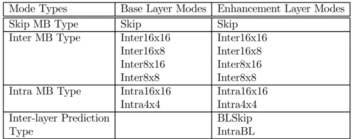
Firstly, the exhaustive search scheme for MLEC is time-consuming, even though it has a better tradeoff between the coding efficiency of two SNR-scalable layers. With our weighting factor w, the encoding process produces a weighted SVC bit-stream composed of two CGS layers. The test mode space is documented in Table 3.1. From this table, we know that there are 56 combinations of the BL mode and the EL mode in exhaustive search scheme for MLEC, the time complexity of encoding is very considerable. To verify this intuition, extensive simulation experiments were conducted by using different video sequences as listed in Table 3.2. The MLEC requires approximately 9 times the computations of the BUEC, and because of this extremely high complexity, we needed to develop a fast mode decision algorithm.

(30)

Table 3.1: Test mode space

Mode Types Base Layer Modes Enhancement Layer Modes

Skip MB Type Skip Skip

Inter MB Type Inter16x16 Inter16x16

Inter16x8 Inter16x8

Inter8x16 Inter8x16

Inter8x8 Inter8x8

Intra MB Type Intra16x16 Intra16x16

Intra4x4 Intra4x4

Inter-layer Prediction BLSkip

Type IntraBL

Table 3.2: Test video sequences

QCIF Sequence CIF Sequence

Soccer Soccer Foreman Foreman Football Football Mobile Mobile Crew Crew Harbour Ice

Secondly, the settings of our analysis were made for several purposes. In order to analyze the combined mode pair distribution from the hierarchical point of view, we classified all possible mode combinations into several classes. Here, the "dominant mode pair" of a class is defined to be the highest representative combination in that class. The R-D cost of dominant mode pair for each class is checked first and then the other possible combinations in the class are compared, of which the cost of the dominant mode pair is minimum. Thus, the dominant mode pair of each class needs to be chosen for the highest probability of minimum R-D cost. Also, in order to develop a fast algorithm with the same level of computation complexity at the BUEC, the mode combinations are classified in a bottom-up manner; the BL mode is decided first and the EL mode decided later. In addition, in order to guarantee the BL R-D performance, Table 3.3 shows the classification according to the BL modes.

Because of the above motivations, we need to determine a "dominant EL mode" of each class, which is combined with the BL mode to be a dominant mode pair. Here,

(31)

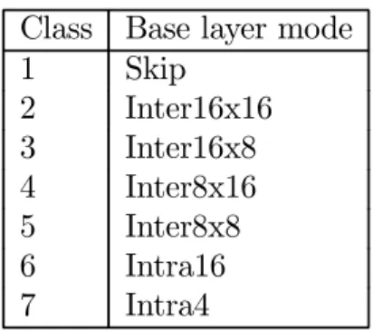
Table 3.3: The MLEC classes

Class Base layer mode

1 Skip 2 Inter16x16 3 Inter16x8 4 Inter8x16 5 Inter8x8 6 Intra16 7 Intra4

Table 3.4: The EL dominant mode for each class

Class (BL mode) _{EL dominant mode (w < 0.5, w ≥ 0.5)}

1 (Skip) (Skip, Inter16x16)

2 (Inter16x16) (Skip, BLSkip)

6 (Intra16) (Skip, Inter16x16)

7 (Intra4) (Skip, Inter16x16)

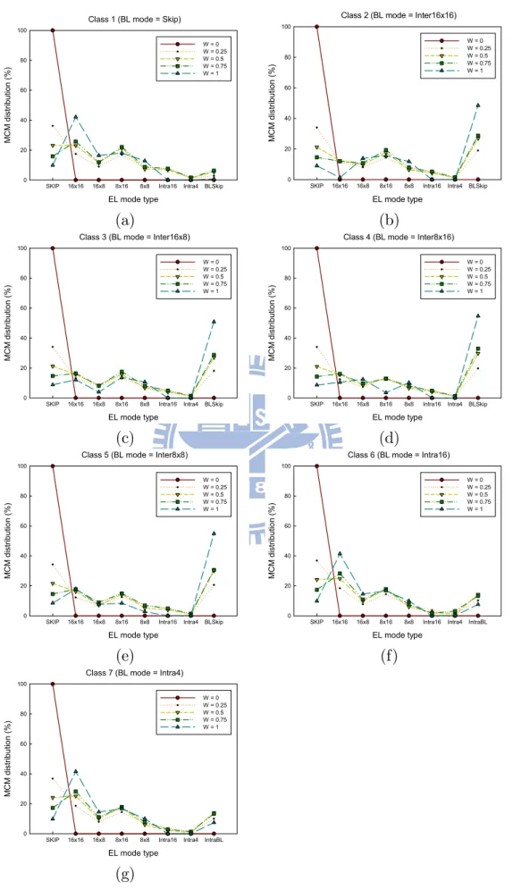
we define a word "MCM" (minimum cost mode) to be the mode type of the EL, and the R-D cost of which is minimum. In this case, a mode type is selected with highest probability of being MCM as the dominant EL mode for each class. In full search scheme, the total 56 combinations are checked for all MBs. Hence, we classified these combinations into seven classes according to the BL modes, and analyze their MCM distributions for each class. Figure. 3.1 shows the MCM distributions for each class. From this figure, two important observations can be made:

1. Compare the curves produced with diﬀerent settings of w in parts (a)(f)(g), the percentage of Skip mode is highest in w < 0.5 cases. However, the percentage of Inter16x16 mode is highest in w ≥ 0.5 cases.

2. Compare the curves produced with diﬀerent settings of w in parts (b)(c)(d)(e), the percentage of Skip mode is highest in w < 0.5 cases. However, the percentage of BLSkip mode is highest in w ≥ 0.5 cases.

Thus, the dominant EL modes are determined for each class according to our obser-vations, and they are summarized in Table 3.4. In such grouping process, the dominant mode pairs involved in each class are first required to be checked.

(32)

Class 1 (BL mode = Skip)

EL mode type

SKIP 16x16 16x8 8x16 8x8 Intra16 Intra4 BLSkip

M C M di st ri but ion (% ) 0 20 40 60 80 100 W = 0 W = 0.25 W = 0.5 W = 0.75 W = 1

Class 2 (BL mode = Inter16x16)

EL mode type

M C M di st ribution (%) 0 20 40 60 80 100 W = 0 W = 0.25 W = 0.5 W = 0.75 W = 1 (a) (b)

EL mode type

M C M di st ribut ion (% ) 0 20 40 60 80 100 W = 0 W = 0.25 W = 0.5 W = 0.75 W = 1

EL mode type

M C M di st ribut ion (% ) 0 20 40 60 80 100 W = 0 W = 0.25 W = 0.5 W = 0.75 W = 1 (c) (d)

EL mode type

M C M di st ribut ion (% ) 0 20 40 60 80 100 W = 0 W = 0.25 W = 0.5 W = 0.75 W = 1

Class 6 (BL mode = Intra16)

EL mode type

SKIP 16x16 16x8 8x16 8x8 Intra16 Intra4 IntraBL

M C M di st ribut ion (% ) 0 20 40 60 80 100 W = 0 W = 0.25 W = 0.5 W = 0.75 W = 1 (e) (f)

Class 7 (BL mode = Intra4)

EL mode type

M C M di st ribut ion (% ) 0 20 40 60 80 100 W = 0 W = 0.25 W = 0.5 W = 0.75 W = 1 (g)

(33)

Additionally, Figure 3.2 (a) presents the "representativeness" of the dominant mode

pairs. The Pa(c, m) is computed as following:

• Ia(c, m1, m2): the R-D cost of dominant mode pair miis minimum in class c.(i = 1

for w < 0.5 cases and i = 2 for w ≥ 0.5 cases)

• Pa(c, m1, m2): the number of MBs, which conform with the event Ia(c, m1, m2) /

the number of total MBs * 100%.

In Figure 3.2 (a), we encode all the MBs with the same class, thus the sequence is encoded seven times. We observed that the representativeness decreases from w = 0 to w = 0.5. For example, the cost of the Skip_Skip (BL_EL) mode pair is minimum in the case of w = 0 and class 1 for every MB. When the weighting factor w increases from 0 to 0.5, the percentage of the dominant mode pair (Skip_Skip) drops to 23.13%. In addition, the percentage of the dominant mode pair (Skip_Inter16x16) increases to 42.12% when the weighting factor w increases from 0.5 to 1. The other classes also have the same tendency of their dominant mode pairs; namely, the dominant mode pair is highly representative with low weighting factor, and the representative property in w = 0.5 case is lowest. In this observation, the tendency also points out that the higher weighting cases seem to be less representative than lower weighting cases (under 50%).

Fortunately, there is another observation, which can remedy the lower representative property in high weighting cases. Table 3.5 presents the comparison results of the dominated mode pairs, and the sums of values for each vertical column are 100%. The

Pb(c, m) is computed as following:

• Ib(c, m1, m2): in the R-D cost comparison of the dominant mode pairs, the cost

of dominant mode pair mi of class c is minimum.(i = 1 for w < 0.5 cases and

i = 2 _{for w ≥ 0.5 cases)}

• Pb(c, m1, m2): the number of MBs, which conform with the event Ib(c, m1, m2) /

the number of total MBs * 100%.

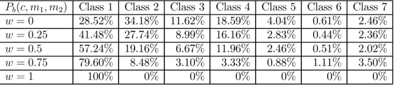
By observing this table and the case of w = 0, 28.52% MBs to selected Skip_Skip as their best combined mode pair; it means that there is 28.52% probability to be classified into class 1 after such grouping process. Additionally, Figure 3.2 (b) shows the tendency of distribution according to Table 3.5. From this figure, we observed that more MBs have a higher probability to be classified into class 1 when the weighting factor increases

(34)

Table 3.5: The comparison results of dominant mode pairs in SOCCER sequence

Pb(c, m1, m2) Class 1 Class 2 Class 3 Class 4 Class 5 Class 6 Class 7

w = 0 28.52% 34.18% 11.62% 18.59% 4.04% 0.61% 2.46% w = 0.25 41.48% 27.74% 8.99% 16.16% 2.83% 0.44% 2.36% w = 0.5 57.24% 19.16% 6.67% 11.96% 2.46% 0.51% 2.02% w = 0.75 79.60% 8.48% 3.10% 3.33% 0.88% 1.11% 3.50% w = 1 100% 0% 0% 0% 0% 0% 0% Soccer QCIF 15Hz Weight W0 W0.25 W0.5 W0.75 W1 Pa (c , m1 , m 2 ) (% ) 0 20 40 60 80 100 (1, Skip, Inter16x16) (2, Skip, BLSkip) (3, Skip, BLSkip) (4, Skip, BLSkip) (5, Skip, BLSkip) (6, Skip, Inter16x16) (7, Skip, Inter16x16) Soccer QCIF 15Hz Weight W0 W0.25 W0.5 W0.75 W1 Pb (c , m 1 , m 2 ) (% ) 0 20 40 60 80 100 (1, Skip, Inter16x16) (2, Skip, BLSkip) (3, Skip, BLSkip) (4, Skip, BLSkip) (5, Skip, BLSkip) (6, Skip, Inter16x16) (7, Skip, Inter16x16)

(a) The representativeness of the (b) The comparison results of the

dominant mode pairs of each class dominant mode pairs of each class

Figure 3.2: The analysis of combined mode pair distribution.

from 0 to 1. In this observation, we found that the low representativeness in the high weighting cases can be remedied by conducting exhaustive mode search for the EL after being grouped into class 1.

In the above analysis, the combined mode pair distributions in MLEC have been discussed detailed. Furthermore, another analysis of cross-layer mode decisions is de-tailed in the next section.

3.2.2 Analyses of Cross-Layer Mode Decision

The analyses in this section are to observe the relationship about cross-layer mode decisions; namely, what the EL modes are selected for a determined BL mode in the exhaustive search scheme. Further insight into the MLEC tradeoﬀ eﬀects of cross-layer mode decisions is obtained by looking at Figure 3.3, which displays the distribution of the BL modes and the distribution of the EL modes in part (a) and (b)∼(h), respec-tively. In part (b)∼(h), the distributions can be seen as the conditional probability of

(35)

the EL modes for a given BL mode. From the figure, several important observations can be made:

1. Compare the curves produced with diﬀerent settings of w in part (a). The larger the value of w, the higher the percentage of the Skip mode; namely, when the optimization degree of EL increases, the allocated bit-rates of the BL decrease. 2. Compare the curves produced with diﬀerent settings of w in part (b). The larger

the value of w, the higher the percentages of the Inter prediction modes; namely, when the optimization degree of EL increases, the usage of the Inter prediction modes increases.

3. Compare the distributions of diﬀerent mode types in part (a). In the all w set-tings, the percentages of Inter8x8, Intra16, and Intra4 are extremely low. Thus, our experimental setting of disabling the finer partition modes than Inter8x8 in the BL is reasonable.

4. Compare the curves produced with diﬀerent settings of w in parts (b)∼(h). The larger the value of w, the lower the percentage of the Skip mode; namely, when the optimization degree of EL increases, the allocated bit-rates of the EL increase. 5. Compare the distributions of the Skip mode and the BLSkip mode in parts (c)∼(f). In all w settings, the percentages of the BLSkip mode are almost the same and larger than 40%. Besides, in the case of w = 0, all the EL modes are Skip mode regardless of their classes. (the Skip mode has 100%) Thus, the Skip mode and BLSkip mode, which are combined with all inter modes, must be checked.

6. Compare the distributions of diﬀerent mode types in part (c). The sum of the percentages of Inter16x16 ∼ Inter8x8 modes is more than 50%, but the percent-ages of the intra prediction modes (Intra16 and Intra4) are extremely low; namely, when the BL mode is Inter16x16, all inter prediction modes must be checked . 7. Compare the distributions of diﬀerent mode types in parts (d)(e)(f). The sum of

percentages of the finer EL modes, the partition of which is smaller than their corresponding BL mode, is more than the other inter prediction modes except for some high weighting cases, but the intra prediction modes (Intra16 and Intra4) still have extremely few percentages. Thus, the finer inter prediction modes combined with their BL modes must be checked.

(36)

BL mode Distribution

BL mode type

SKIP 16x16 16x8 8x16 8x8 Intra16 Intra4

B L M ode dist rib ut ion ( % ) 0 20 40 60 80 100 W = 0 W = 0.25 W = 0.5 W = 0.75 W = 1 BL mode = Skip EL mode type

E L M ode dist rib ut ion ( % ) 0 20 40 60 80 100 W = 0 W = 0.25 W = 0.5 W = 0.75 W = 1 (a) (b) BL mode = Inter16x16 EL mode type

E L M ode dist rib ut ion ( % ) 0 20 40 60 80 100 W = 0 W = 0.25 W = 0.5 W = 0.75 W = 1 BL mode = Inter16x8 EL mode type

E L M ode dist rib ut ion ( % ) 0 20 40 60 80 100 W = 0 W = 0.25 W = 0.5 W = 0.75 W = 1 (c) (d) BL mode = Inter8x16 EL mode type

E L M ode dist rib ut ion ( % ) 0 20 40 60 80 100 W = 0 W = 0.25 W = 0.5 W = 0.75 W = 1 BL mode = Inter8x8 EL mode type

E L M ode dist rib ut ion ( % ) 0 20 40 60 80 100 W = 0 W = 0.25 W = 0.5 W = 0.75 W = 1 (e) (f) BL mode = Intra16 EL mode type

E L M ode dist rib ut ion ( % ) 0 20 40 60 80 100 W = 0 W = 0.25 W = 0.5 W = 0.75 W = 1 BL mode = Intra4 EL mode type

E L M ode dist rib ut ion ( % ) 0 20 40 60 80 100 W = 0 W = 0.25 W = 0.5 W = 0.75 W = 1 (g) (h)

Figure 3.3: Cross-layer mode pair distribution in diﬀerent weighting cases in

(37)

Sec 3.3. Fast Mode Decision Algorithm

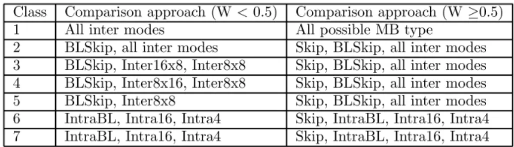
Table 3.6: The candidate mode pairs for the EL refinement process.

Class Comparison approach (W < 0.5) _{Comparison approach (W ≥0.5)}

1 All inter modes All possible MB type

2 BLSkip, all inter modes Skip, BLSkip, all inter modes

3 BLSkip, Inter16x8, Inter8x8 Skip, BLSkip, all inter modes

4 BLSkip, Inter8x16, Inter8x8 Skip, BLSkip, all inter modes

5 BLSkip, Inter8x8 Skip, BLSkip, all inter modes

6 IntraBL, Intra16, Intra4 Skip, IntraBL, Intra16, Intra4

7 IntraBL, Intra16, Intra4 Skip, IntraBL, Intra16, Intra4

8. Compare the distributions of diﬀerent mode types in parts (g)(h). The percentage of the IntraBL mode is extremely larger than other inter prediction modes. Thus, the IntraBL mode combined with their BL modes must be checked.

9. Observe the w = 1 case in parts (b)∼(h), because w = 1 optimizes for the EL, the BL mode of all MBs are selected to be Skip mode. Thus, we can’t see the curves of the w = 1 case in these figures.

In this section, the relationship of cross-layer mode decisions in MLEC has been detailed. Thus, according to these important observations from Subsection 3.2.1 and Subsection 3.2.2, a fast mode decision algorithm is developed, and the details of which are discussed in the next section.

3.3 Fast Mode Decision Algorithm

According to the analysis in Subsection 3.2.2, the candidate mode pairs for the EL refinement process are defined. It is shown in Table 3.6, the class 1 compares all possible EL modes to ensure the R-D performances of high weighting factor cases, and class 6 and class 7 compare the all intra prediction modes. The finer partition modes, partition size of which are smaller than the corresponding BL mode, are compared in the low weighting factor cases of classes 2 ∼ 5.

Figure 3.4 shows the flowchart of the proposed fast mode decision algorithm. A summary of the proposed fast mode decision algorithm is provided as follows:

1. Compute the MLEC-RD cost for the dominant mode pairs after the EL dominant mode assignment process.

2. Choose the dominant mode pair with minimum cost as the best prediction mode pair.

(38)

Start

Select the one that yields the minimum MLEC RD cost as the best mode pair

End

Base = Intra Base = Inter

Base = Skip

Stage 2: Decide the EL mode

BL mode = Inter16x16 w < 0.5 ? BL mode is Inter mode? EL dominant mode is Inter16x16

Compare the MLEC-RD cost of the dominant mode pairs of class 1~7 EL dominant

mode is Skip mode is BLSkipEL dominant

No

Yes Yes

Stage1: Decide the BL mode

BL mode =

Skip BL mode =Inter16x8 BL mode =Inter8x16 BL mode =Inter8x8 Intra4 or Intra16BL mode =

Class 1 Class 2 Class 3 Class 4 Class 5 Class 6, 7

Check BLSkip, 16x8, 8x8 Check all inter

modes Check BLSkip, allinter modes Check BLSkip,8x16, 8x8 Check BLSkip,8x8 Check IntraBL,Intra16, Intra4

(W<0.5)

Figure 3.4: The flowchart of the proposed fast mode decision algorithm.

• When the weighting factor increases up to 1, the process has higher proba-bility to go to the class 1(Skip_Skip) branch.

• When the weighting factor decreases down to 0, the process is high repre-sentative for each class.

3. After deciding the best dominant mode pair of current ML-MB pair in stage 1, the mode decision process proceeds to stage 2 to check the other possible EL modes.

4. If the BL mode is chosen to be Skip mode in stage 1, all inter modes for the EL mode are checked in stage 2 when w < 0.5, while all possible combinations for the EL mode are checked in stage 2 when w ≥ 0.5. (In order to ensure no significant R-D performance loss in high weighting case.)

5. If the BL mode is chosen to be Inter mode in stage1, the finer partition modes or all inter modes according to Table 3.6 for the EL mode are checked in stage2.

(39)

Sec 3.4. Summary

Table 3.7: The number of checked mode pairs in average.

Weight Soccer Football Foreman Mobile Harbour Ice Crew

w = 0 11.05 10.51 11.0 10.73 10.98 11.49 11.21 w = 0.25 12.42 11.23 12.12 11.08 11.84 11.99 12.27 w = 0.5 12.50 11.24 12.69 11.63 12.47 11.64 12.72 w = 0.75 12.92 11.94 12.85 12.93 13.42 13.29 13.26 w = 1 14.00 14.00 14.00 14.00 14.00 14.00 14.00 Average 12.58 11.78 12.53 12.07 12.54 12.48 12.69

(In order to reduce the time complexity.)

6. If the BL mode is chosen to be Intra mode in stage1, only Skip, IntraBL, and all intra modes for the EL mode are checked in stage2. (In order to reduce the time complexity.)

7. After checking the EL mode in stage 2, selecting the one that yields the minimum MLEC RD cost as the optimal mode pair, and the mode decision process proceeds to the next ML-MB pair.

From the algorithm flowchart in Figure 3.4 and the test mode space in Table 3.1, we see that the critical path of the fast algorithm is the path of choosing the class 1 as the best mode pair when w ≥ 0.5, which need to check 14 possible combinations totally. In order to calculate more accurately for the number of combinations to be checked in the fast algorithm, we run the algorithm for diﬀerent sequences and computing the average checked mode pairs per ML-MB pair. It is shown in Table 3.7. With this table, we proved that we reduced the test mode set from 56 combinations to

11.78 _{∼ 12.69 combinations per ML-MB in average, which can achieve the speed of}

BUEC theoretically.

3.4 Summary

In this chapter, a fast mode decision algorithm is exploited for searching the MLEC R-D optimal mode pair for each ML-MB pair based on a series of mode distribution analyses. For achieving the bottom-up encoding speed, the development for fast algorithm is necessary due to the high complexity of the exhaustive search scheme. Because of the observations of our analyses, the proposed algorithm ensures the R-D performance for all weighting cases, and a good candidate mode pair space of the EL is defined according

(40)

to these data support. Hence, this two-stage algorithm can improve eﬀectively our encoding speed.

We also reveal the effectiveness of the fast algorithm by analyzing the average checked mode pairs. The excellent co-working of two stages promises the goodness of chosen mode pair. The effectiveness of each stage heavily depends on the MLEC approaches and the property of the inter-layer predictions. To satisfy the effectiveness of each stage ensures that the optimal R-D performance can be achieved. In the next chapter, we introduce the analysis of time complexity, implementation settings of encoding parameters to produce weighted SVC bit-streams for efficient MLEC, and the details of R-D performance comparison.

(41)

CHAPTER 4 Experiments and Analyses

4.1 Implementation and Test Conditions

The proposed fast mode decision scheme and the exhaustive search scheme have been implemented with the JSVM 9.12.2 [7]. Several QCIF-format and CIF-format test sequences, covering a wide range of spatio-temporal characteristics are used. All the experiments were conducted on a PC equipped with a 2.6GHz Intel Quard-core proces-sor and 12 GB memory. The test conditions are detailed as follows:

1. For each test sequence, 31 frames are encoded with the group of picture (GOP) structure IPPP...and a frame rate of 15Hz.

2. Two CGS layers are used.

3. Because the Lagrangian multiplier λi for each layer i needs to be modified for

MLEC [8]. We fixed the BL QPB and determined the EL QPE iteratively to meet

the quality constraints by using the "FixedQpEncoderStatic" program provided in [7]. The details are presented in Section. 4.3.

4. The initial quantization parameters (QP) of the "FixedQpEncoderStatic" pro-gram were set as follows:

(42)

Chapter 4. Experiments and Analyses

• The QPE was set to 28.

• The QPB was set to QPB = QPE+ 6.

5. The RDO is enabled.

6. The CAVLC entropy coding is used.

7. For Inter prediction, only Inter16x16, Inter16x8, Inter8x16, and Inter8x8 are enabled.

8. The motion estimation is conducted with consideration of MLEC as presented in Eq. (3.3).

9. The inter-layer residual prediction is enable.

4.2 R-D Tradeoﬀ with Fixed QP Setting

4.2.1 Schwarz’s MLEC

The MLEC proposed by Schwarz et al. have been implemented in SVC reference software. The QP settings are as follows:

• The QPE was set to 28.

• The QPB was set to QPB = QPE + 4.

According to the Eq. (2.4), and the minimization process in Section. 2.2.2.1, the exhaustive search scheme and the fast search scheme are reconstructed. Additionally, the candidate mode pairs of Schwarz’s fast search scheme are chosen by analyzing the mode distribution of exhaustive search scheme in SOCCER sequence. 24 combina-tions of the candidate mode pairs are shown in Table. 4.1. Also, Table. 4.2 shows the R-D comparisons between these schemes. The following performance indexes are used in that table: the weighting factor w [0, 1] controls the trade-oﬀ between the BL and the EL coding eﬃciency. The higher the value w is, the more the weighting

is allocated to EL; ∆PSNR means the average PSNR changes (in dB)1; ∆Bit-Rate

means the total bit rate changes (in percentage)2_{; ∆T means the average time saving}

(in percentage)3; "+" means increase; and "-" means decrease. These performance

indexes will be used continuously in the Section 4.4. The weighting factor w varies over the set {0, 0.25, 0.5, 0.75, 1}. When w equals to 0, it represents the JSVM encoder

1_{∆PSNR = Y-PSNR of fast search scheme − Y-PSNR of exhaustive search scheme}

2_{∆Bit-Rate (%) =} Bit-rate of fast search schem e - Bit-rate of exhaustive search schem e

(43)

Sec 4.2. R-D Tradeoﬀ with Fixed QP Setting

Table 4.1: Candidate mode pairs of Schwarz’s fast scheme

Base Layer Modes Enhancement Layer Modes

Skip Skip, BLSkip, Inter16x16, Inter16x8, Inter8x16, Inter8x8

Intra16x16, Intra4x4

Inter16x16 Skip, Inter16x16, BLSkip

Intra16x16 Skip, IntraBL

Intra4x4 Skip, IntraBL

Table 4.2: RD comparison of Schwarz’s MLEC in soccer sequence

Base layer Enhancement layer Time

CIF w ∆PSNR (dB) ∆Bit-Rate (%) ∆PSNR (dB) ∆Bit-Rate (%) ∆T (%)

0 0 0 -0.04 0.30 -73.46

0.25 0 -0.40 -0.04 -0.36 -73.19

SOCCER 0.5 +0.02 +0.10 +0.02 -0.16 -72.63

0.75 -0.01 +0.31 -0.02 -0.73 -73.04

1 0 0 0 0 -73.26

control, but on the other hand, it trades oﬀ the BL and the EL coding eﬃciency in both the search criteria when w is greater than 0.

Figure. 4.1 shows that the fast search scheme has a similar R-D performance as that of the exhaustive search scheme. The rate-distortion curves are compared with

that of single-layer coding. The single-layer curve is experimented with the fixed QPB

and QPE settings. With the JSVM encoder control corresponding to w = 0, the BL

coding efficiency is virtually identical to that of single-layer coding. By increasing w, the EL coding efficiency can be improved while introducing a loss of the BL coding efficiency.

After our implementation of Schwarz’s MLEC, we found that there is a problem when testing the higher weighting cases. This problem is shown in Figure. 4.2. In this figure, the BL R-D performance decreases with the increment of w, because the opti-mization for the BL decreases. However, the EL R-D tradeoﬀ becomes unpredictable as presented by the arrow lines named from 1 to 3. The tradeoﬀ from w = 0.9 to w = 0.99 is in the reverse direction (arrow line 2); namely, we can’t obtain the expected R-D performance in EL when we set w to higher values. The cause of this problem is that the weighting factor w is involved in the constraints of Schwarz’s objective optimiza-tion problem. The EL constraint is unlimited when w = 0, but it gradually converges

(44)

Chapter 4. Experiments and Analyses Soccer CIF 30Hz Bite rate[kbits/s] 0 200 400 600 800 1000 1200 Y -PSN R [dB] 31 32 33 34 35 36 37 Single layer(Qp32-Qp28) JSVM Multi-layer(W = 0) Multi-layer(W = 0.25) Multi-layer(W = 0.5) Multi-layer(W = 0.75) Multi-layer(W = 1) Soccer CIF 30Hz Bite rate[kbits/s] 0 200 400 600 800 1000 1200 Y -PSN R [dB] 31 32 33 34 35 36 37 Single layer(Qp32-Qp28) JSVM Multi-layer(W = 0) Multi-layer(W = 0.25) Multi-layer(W = 0.5) Multi-layer(W = 0.75) Multi-layer(W = 1)

(a)Exhaustive search scheme (b)Fast search scheme

Figure 4.1: The RD curves of Schwarz’s MLEC with fixed QP setting.

Socc er CIF 30Hz Bite rate[kbits/s] 0 2 00 40 0 60 0 800 10 00 120 0 Y-P SN R [d B ] 3 1 3 2 3 3 3 4 3 5 3 6 3 7 Sing le laye r(Q p32 -Qp2 8) JSVM Multi-layer(W = 0) Multi-layer(W = 0.25) Multi-layer(W = 0.5) Multi-layer(W = 0.75) Multi-layer(W = 0.9) Multi-layer(W = 0.95) Multi-layer(W = 0.99) Multi-layer(W = 1) Y-PSN R [d B] Bit-rate[kbits/s] 1 2 3

Figure 4.2: The RD curves of the higher weighting cases.

to target bit-rate of the EL while increasing the weighting factor w. Therefore, the bit-rates contributed from the BL are not suﬃcient to support the usage of the EL.

In order to see the further insight into the relationship between the R-D tradeoﬀ and the constraints of Schwarz’s objective optimization problem, the following frame level analyses are made. Several statistic terms are defined in our analyses:

δr(i, w1, w2) = M −1_X n=0 (Ri(w2, n)− Ri(w1, n)) δd(i, w1, w2) = M −1_X n=0 (Di(w2, n)− Di(w1, n))

(45)

Sec 4.2. R-D Tradeoﬀ with Fixed QP Setting

δR(w1, w2) =

M −1_X

n=0

((R0(w2, n) + R1(w2, n))− (R0(w1, n) + R1(w1, n)))

n is the MB address, and M is the number of MBs in a frame. Ri(w1, n) means

the bits of nth MB of layer i in w = w1 case for MLEC. Also, Di(w1, n) means the

distortion of nth MB of layer i in w = w1 case for MLEC (i = 0 for the BL, i = 1 for

the EL). Likewise, Ri(w2, n) and Di(w2, n)are computed in w = w2 case. Because the

values of δr(i, w1, w2), δd(i, w1, w2), and δR(w1, w2)are too huge to be observed clearly,

another three terms are defined as follows:

˜

δr(i, w1, w2) ={

− log10|δr(i, w1, w2)| if δr(i, w1, w2) < 0

log10|δr(i, w1, w2)| if δr(i, w1, w2) > 0

˜

δd(i, w1, w2) ={

− log10|δd(i, w1, w2)| if δd(i, w1, w2) < 0

log₁₀_|δd(i, w1, w2)| if δd(i, w1, w2) > 0

˜

δR(w1, w2) ={

− log10|δR(w1, w2)| if δR(w1, w2) < 0

log10|δR(w1, w2)| if δR(w1, w2) > 0

By the above equations, ˜δr(i, w1, w2)can be seen as the alteration degree of the

bit-rate of layer i with the changing of w. In the meantime, ˜δd(i, w1, w2) can be regarded

as the alteration degree of distortion of layer i with the changing of w, while ˜δR(w1, w2)

can be seen as the alteration degree of total bit-rate with the changing of w. When the alteration degree is far less than 0, it means that the negative growth increases with the changing of w. However, it stands for the increment of the positive growth when the alteration degree is far greater than 0. Figure 4.3 shows the analysis of these alteration degrees in the Schwarz’s MLEC. Parts (a)(b) represent the alteration degrees of the BL, parts (c)(d) the alteration degrees of the EL, and part (e) the alteration degrees of the total bit-rate. From this Figure, several important observations are immediate: 1. Compare the curves produced with diﬀerent settings of w in parts (a)(b). In

all weighting cases, the alteration degrees of R0 are negative growth, and the

alteration degrees of D0 are positive growth, since the optimization of the BL

decreases. By increasing w, the negative growth of R0 increases while increasing

針對可調視訊編碼多層編碼控制的快速決策演算法

國

立

交

通

大

學

資訊科學與工程研究所

碩

士

論

文

針對可調視訊編碼多層編碼控制的

快速決策演算法

A Fast Mode Decision Algorithm for SVC Multi-Layer

Encoder Control

研 究 生：林哲永

指導教授：彭文孝 教授

針對可調視訊編碼多層編碼控制的快速決策演算法

A Fast Mode Decision Algorithm for SVC Multi-Layer Encoder Control

研 究 生：林哲永 Student：Jhe-Yong Lin

指導教授：彭文孝 Advisor：Wen-Hsiao Peng

國 立 交 通 大 學

資 訊 科 學 與 工 程 研 究 所

碩 士 論 文

針對可調視訊編碼多層編碼控制的快速決策演算法

研 究 生：林哲永 指導教授：彭文孝

國立交通大學資訊科學與工程研究所 碩士班

摘

要

A Fast Mode Decision Algorithm for SVC

Multi-Layer Encoder Control

Student : Jhe-Yong Lin Advisor : Wen-Hsiao Peng

Institute of Computer Science and Engineering

National Chiao Tung University

ABSTRACT

誌

謝

Contents

List of Tables

List of Figures

CHAPTER 1

Introduction

1.1

Background

I

P

P

1.2

Problem Statement

1.3

Contributions

1.4

Organization

CHAPTER 2

Scalable Video Coding and its Encoder

Control

2.1

Introduction to SVC

2.1.1

Concept

2.1.2

Inter-Layer Prediction

2.2

SVC Encoder Control

2.2.1

Bottom-up Encoder Control

2.2.2

Multi-layer Encoder Control

2.3

Comparison and Summary

CHAPTER 3

Fast Mode Decision for Multi-layer Encoder

Control

3.1

Proposed Multilayer Encoder Control

3.2

Analysis of Mode Distribution

3.2.1

Combined Mode Pair Distribution in MLEC

研究生：林哲永

指導教授：彭文孝教授

研究生：林哲永 Student：Jhe-Yong Lin

國立交通大學

資訊科學與工程研究所

碩士論文

研究生：林哲永指導教授：彭文孝

國立交通大學資訊科學與工程研究所碩士班