量化MIMO系統通道容量之研究與分析

1

國

立

交

通

大

學

電子工程學系 電子研究所碩士班

碩

士

論

文

量化 MIMO 系統通道容量之研究與分析

Research and Analysis in Channel Capacity of

Quantized MIMO System

研 究 生：黃 俞 榮

指導教授：桑 梓 賢 教授

1

量化 MIMO 系統通道容量之研究與分析

Research and Analysis in Channel Capacity of Quantized

MIMO System

研 究 生：黃俞榮 Student：Yu-Rong Huang

指導教授：桑梓賢 教授 Advisor：Tzu-Hsien Sang

國 立 交 通 大 學

電子工程學系 電子研究所碩士班

碩 士 論 文

Submitted to Department of Electronics Engineering & Institute of Electronics

College of Electrical and Computer Engineering

National Chiao Tung University

in Partial Fulfillment of the Requirements

for the Degree of

Master

in

Electronics Engineering April 2009

Hsinchu, Taiwan, Republic of China

I

量化 MIMO 系統通道容量之研究與分析

研究生：黃俞榮 指導教授：桑梓賢 教授

國立交通大學

電子工程學系電子研究所碩士班

摘要

要的好處為增加頻寬效益(spatial multiplexing)和對抗通道衰減(spatial diversity),但

過去對於 MIMO 系統的研究， 甚少考慮接收端量化的問題,在實際的應用上,發射

及接收的信號都是離散訊號。在這篇論文中,我們主要研究接收訊號經過量化

後,MIMO 系統的通道容量，並且考慮簡單的 Relay Channels。

我們首先提出在傳送訊號有功率限制的情況下，且接收訊號經過量化的通道 容量計算演算法,並且經由分析其最佳輸入信號的機率分布,說明且驗證演算法的 正確性,接著用我們所提出的演算法模擬在不同的 MIMO 架構中所得到的通道容 量且說明其結果,並且在傳送天線數以及調變信號固定的情況下,討論 AGC 使其 可以得到最大的消息量。最後,我們分析簡單的 relay channel 經過量化後的通道容 量。

II

Research and Analysis in Channel Capacity of Quantize

MIMO System

Student：Yu-Rong Huang Advisor：Tzu-Hsien Sang

Department of Electronics Engineering & Institute of Electronics

National Chiao Tung University

ABSTRACT

In the past few years, MIMO systems were already proven to have many

advantages. The main advantages are spatial multiplexing and spatial diversity. In the

past research, few have considered the problem of discrete signals at the transmitters

and receivers; in this thesis, we study and analyze the capacity of quantized MIMO

systems and consider the case of simple relays.

We propose an algorithm that can calculate Discrete-input and Quantized-output

channel capacity with input power constraint and analyze the optimal input distribution.

Then we run the algorithm to calculate channel capacity of different MIMO scenarios

and explain the simulation results. Proper AGC scheme is also used to get the

maximum information rate. Finally we consider simple relay channels and the

III

誌

謝

IV

Contents

Chapter 2 An Algorithm for computing the capacity of Discrete Input and Discrete Output MIMO channel with input power constraint ... 9

2.1 Quantized MIMO System ... 9

2.2 Algorithm ... 11

2.2.1 Algorithm Research ... 11

2.2.2 Interval halving procedure ... 13

2.2.3 Newton-Raphson procedure ... 14

2.2.4 Algorithm Convergence ... 14

Chapter 3 Simulation Result ... 15

3.1 Discrete-input and discrete-output MIMO Rayleigh flat-Fading channels ... 15

3.2 The maximum information rate about the discrete-input and discrete-output MIMO channel ... 17

3.3 Optimal input vector distribution for different input power constraint ... 20

V

3.3.1 Low power constraint ... 20

3.3.2 High power constraint ... 26

3.4 AGC to achieve the channel capacity ... 28

Chapter 4 Simple Relay Case ... 30

4.1 Introduction ... 30

4.2 Basic Memoryless Forwarding Strategies ... 31

4.2.1 Demodulate And Forward ... 31

4.2.2 Amplify And Forward ... 31

4.3 Simulation Results ... 32 Bibliography 36

VI

List of Figures

Fig. 1.1 Digital input and continued output AWGN channel model [4]…….2

Fig. 1.2 An uniform quantizer………3

Fig. 1.3 Simulation of 4X4 MIMO,4-QAM modulation. Result for different resolution of quantization is shown [7]………5

Fig. 1.4 Quantized MIMO system model [7]………5

Fig. 2.1 Quantized MIMO system model [7]………..10

Fig. 3.1 Simulation Results………...16

Fig. 3.2 All possible transmit signal vectors in 2X2 quantized MIMO system………18

Fig. 3.3 Quantized signal vectors at the receiver………18

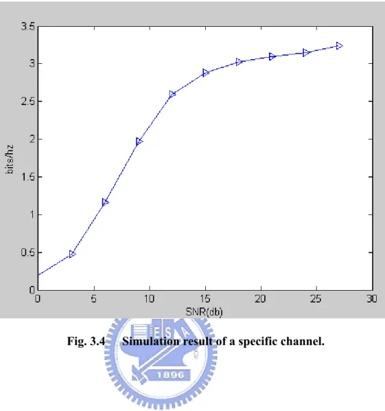
Fig. 3.4 Simulation result of a specific channel………...19

Fig. 3.5 Simulation result for low input power constraint……….23

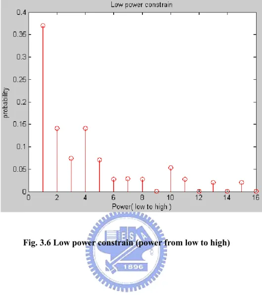
Fig. 3.6 Low power constrain (power from low to high)………24

Fig. 3.7 Optimal input distribution for high power constraint……….26

Fig. 3.8 High power constrain (power from low to high)………..27

Fig. 3.9 Different AGC……….29

Fig. 4.1 Elementary Relay Channel……….30

Fig. 4.2 Different Parallel Relay………...33

VII

Fig. 4.4 Different Relay Strategies………..34

Fig. 4.5 Different Received Antenna………..34

Fig. 4.6 Different Combination………..35

VIII

List of Tables

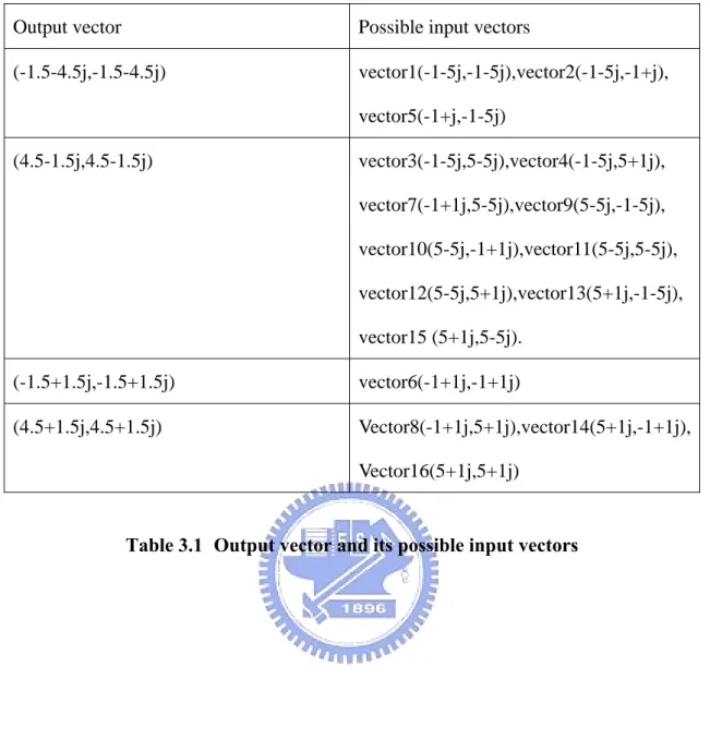
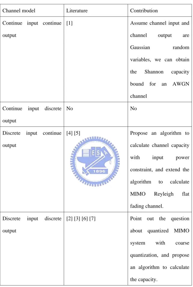
Table 1.1 Literature summary………7 Table 3.1 Output vector and its possible input vectors……….25

1

Chapter 1

Introduction

1.1 Motivation

Channel capacity, a fundamental concept in information theory, was introduce by

Shannon [1] to specify the asymptotic limit on the maximum rate C at which

information can be reliable conveyed by the channel. Any coding scheme that

superficially appears to operate at a rate higher than C will cause enough data to be

lost because of uncorrectable channel errors so that the actual information rate is not

to be greater than C.

In [1], when computing the channel capacity the assumption is made that the

channel inputs and the channel outputs can be treated as continues random variables.

Since the DSP hardware used in digital modems utilizes a finite signal set (channel

input are modulation signals, such as QAM signals), and channel output are quantized

signals, it is clear that the channel inputs and the channel outputs are not Gaussian

random variables and the Shannon bound is not exact. So our research motivation is

to propose an algorithm to modify the Shannon bound in the practical digital channels,

2

1.2 Literature Review

The problem of obtaining the capacity of a discrete-input (fixed input

constellations) and quantized-output (the output signal is quantized by

quantizer )MIMO Rayleigh flat-fading channel has been preceded by such work as

[1], in which Shannon calculated the capacity of an AWGN channel and showed that

this capacity is achievable by a Gaussian input distribution. Arimoto [2] and Blahut

[3] derived a numerical method for computing the capacity of discrete memoryless

channels, but their algorithm did not support input power constraint. In [4], the

Blahut-Arimoto algorithm is modified to incorporate an average power constraint,

and is used to compute the capacity of discrete-input and continuous-output (output

signals are not quantized) channel, and also the convergence is proved. The channel

model in [4] is shown in Fig. 1.1.

Fig. 1.1 Digital input and continued output AWGN channel model [4].

3

calculates the capacity of a discrete-input and continuous-output channel) to

calculate the capacity of a MIMO Rayleigh flat-fading channel, which is also

discrete-input and continuous-output channel. The algorithm becomes very

computationally complex when the number of transmit antennas and signal set size

grow; so the author makes a postulation that the MIMO channel is independent

across antennas and dimensions (real dimension and imaginary dimension). Base on

the postulation, the author proposed a new algorithm which drastically reduces the

computation cost (for example, for 64-QAM constellations and three transmit

antennas, a total of 262143 variables are evaluated in the old algorithm, while only 7

variables in the new algorithm).

In [6], Obianuju Ndili and Tokunbo Ogunfunmi discovered that the Shannon

limit does not exist in modern communication systems (because of the DSP

hardware used in digital modems utilizes a finite signal set), so they proposed the

constrained Blahut-Arimoto algorithm to calculate the channel capacity with

discrete-inputs (the input signals has not been modulated) and quantized outputs (the

output signals was quantized by quantizer, which was shown in Fig. 1.2), and

extended their algorithm to calculate the capacity of MIMO channels, but they did

not prove the convergence of their algorithm.

4

In [7], the author pointed out a question, a 64-QAM modulated signal received

over a time-dispersive SISO (one transmit antenna and one receive antenna) channel

with four multi-path components can very well be quantized by a 8 bit ADC

(4*64=256,log 256 =8), which is sufficiently large for the modem to operate close to ₂

channel capacity. However, the reliance on fine ADC granularity easily becomes

unjustified as soon as MIMO systems come into play. Consider for instance two data

streams (two transmit antenna) of 64-QAM modulated signals received over a

time-dispersive MIMO channel with four multi-path components. Now we need at

least 14 bit (log (4 * 64 * 64)₂ =14) of resolution in order to obtain a fine granular quantization at each receive antenna. With increasing number of transmit antennas,

the ADC resolution needed for fine granular quantization soon becomes infeasible in

practice. But in their simulation (which is shown in Fig. 1.3), they showed that even

coarse quantization leads to channel capacities which are surprisingly close to the

ones obtainable with fine-granularity quantization. Their system model is shown in

Fig. 1.4, where the transmit antennas transmit digital signal (such as QAM and PAM),

and receive antennas quantized the received signals individually. Their method

calculated the channel capacity by calculating the mutual information between X and

Y (X and Y are vector), and letting the input distribution be uniform, shown in (1.1),

so in their simulation, they did not get the optimal input distribution.

1 1 ₁

1

[ |

]

1

[ | ] * ln

[ | ]

pr yi xk

M

C

pr yi xj

M

pr yi xj

= −

∑

∑ ∑

5

Fig. 1.3 Simulation of 4X4 MIMO,4-QAM modulation. Result for different resolution of quantization is shown [7].

6

According to these literatures, we classify the channel into four types.

z Continuous-input and continuous-output

The channel input is an analog random variable, and the channel output is

also an analog random variable.

z Continuous- input and discrete-output

The channel input is an analog random variable, and the channel output is a

discrete random variable (the output signal is quantized by a quantizer).

z Discrete-input and continuous-output

The channel input is a discrete random variable (the input signal is a

modulation signal), and the channel output is an analog random variable.

z Discrete-input and discrete-output

The channel input is a discrete random variable (the input signal is a

modulation signal), and the channel output is also a discrete random variable (the

output signal is quantized by a quantizer).

In the end of this section, we summarize in Table 1.1 the different channel

7

Channel model Literature Contribution

Continue input continue

output

[1] Assume channel input and

channel output are

Gaussian random

variables, we can obtain

the Shannon capacity

bound for an AWGN

channel

Continue input discrete

output

No No

Discrete input continue

output

[4] [5] Propose an algorithm to

calculate channel capacity

with input power

constraint, and extend the

algorithm to calculate

MIMO Reyleigh flat

fading channel.

Discrete input discrete

output

[2] [3] [6] [7] Point out the question

about quantized MIMO

system with coarse

quantization, and propose

an algorithm to calculate

the capacity.

8

1.3 Purpose Of Research

In the previous section, we see that discrete-input and discrete-output channel

model suits digital communication systems, but there is not an algorithm to calculate

this channel capacity with input power constraint and a convergence proof (in [6], the

authors proposed an algorithm, but they can not prove the convergence of the

algorithm. In our simulations, we found case where their algorithm fails to converge.).

Our purpose of research is to propose an algorithm, which can calculate the

discrete-input and discrete-output channel capacity with input power constraint, and

guarantee the algorithm convergent, and the algorithm is extended to MIMO cases.

We use the algorithm to study the optimal input distribution with different input

power constraint. In the end, we hope to use the algorithm to study simple relay

9

Chapter 2

An Algorithm for computing the

capacity of Discrete Input and

Discrete Output MIMO channel

with input power constraint

2.1 Quantized MIMO System

Let us consider the quantized MIMO systems in Fig. 2.1, where nT transmit

antennas are connected to nR receive antennas by the channel matrix H∈CnT nR* ,

which is assumed to be completely known to the transmitter and receiver. Because of

knowing the channel state at the transmitter, we can get the optimal input distribution

which is fitted the input power constraint ( * 2

i

Pi i =Pav

∑

samples ( ,v v_{1 2},...,v_nR) of complex, circularly symmetric, additive, white Gaussian noise of zero mean and variance of σv2/2 in its real and imaginary part, respectively,

yielding total noise power σv2. The receive signal is split up into real-part and

10

output the quantized signals (y y₁, ₂,...,y_2nR). Let us collect the input and output signals into vector

X=[ ,x x_{1 2,}...x_nT]T∈M (2.1)

Y=[ ,y y_{1 2,}...y_2nR]T ∈Q (2.2) Where M is a finite set containing all possible modulated transmit vector X,

while Q is a finite set containing all possible quantized receive vectors Y. Let us

write the input-output relationship of the quantized MIMO system as

Y=Quantized (HX+V) (2.3)

The individual quantizer is defined by their input-output relationship as

Quantized(r ) =q iff _i l q_i( )< ≤r_i u q_i( ) (2.4) Where q is the output of the quantizers when its input ranges between a lower limit

( )

i

l q and an upper limit u q , and these limits define the quantization interval for _i( )

which the quantizers outputs the value q. Here we use the uniform quantizers in our

simulation.

11

2.2 Algorithm

2.2.1 Algorithm Research

Our goal is to find P_X( )⋅ which maximize the information rate I(X;Y|H). Here

I(X;Y|H) is the mutual information between channel input and channel output

assuming the transmitter and receiver knows the channel matrix H.

The discrete-input and discrete-output channel capacity computation problem is stated

as follows:

Find the pmf (probability mass function) that satisfy the following equation

* P ( ) ( ) arg max I( ) P ⋅ ⋅ = X X X;Y | H (2.6)

The maximization in (2.6) is taken under the following set of constraint.

( * i H av MP P ∈ ≤

∑

( ) 1

i M

P

∈ =

∑

Finally, we wish to evaluate C (the discrete-input and discrete-output channel

capacity), defined as

C = I(X; Y |H)|P_X( )⋅ =P_X*( )⋅ (2.9) An algorithm computing the discrete-input and continuous-output channel

capacity has been proposed in [6]. We can regard the discrete-output as a special case

of the continuous-output. With the idea, we propose a discrete-input and discrete-

output version for computing the quantized MIMO channel capacity. We state as

follows.

12

Step1: Initialization

z P_X( )⋅ is chosen as any valid pmf over X=[ ,x x_{1 2,}...x_nT]T (2.10) Step2: Expectation

z For all X_i∈M , compute

[ ( )log (₂ ( ))] ( ) i P T E P P = X|Y i Y X|Y i X i X | Y X | Y X (2.11) Step3: Maximization

z For all X_i∈M , compute

∑

z Where λ is chosen to satisfy

∑

In step2, the value T can be determined from the probability_i P (Y | X) . When _Y|X

given H and X, Y~N (HX, 2

v

σ I), thus knowing the quantization levels and appropriate

decision regions, the complementary error function can be used to compute

Y|X

P (Y | X) .

In step3, λ is chosen to satisfy the specific equation, and we introduce two methods in next two sections.

13

2.2.2 Interval halving procedure

Interval halving procedure is an efficient method for solving equation f(x) =0.

The requirements for using this method is that there are two values x and ₁ x that ₂

satisfy f(x )f(₁ x ) <0 .Since f(₂ x ) and f(₁ x ) have opposite signs, we know by the ₂

intermediate value theorem that there exists a solution x_% and that x₁≤ ≤x_% x₂, and with only n+1 function evaluations we can find a shorter interval of length

1 2 2

n

x x

ε _{= −} −

that contains x%, the procedure was described as follows.

Input: x ,₁ x , f(x),₂ ε (tolerance error)

Output: A solution to the equation f(x) =0 that lies in an interval of length <ε Repeat Set x = (₃ x +₁ x )/2 ₂ If f (x ) f (₃ x ) <0 Then ₁ Set x =₂ x ₃ Else Set x =₁ x ₃ End If Until x₁−x₂ <2ε

14

2.2.3 Newton-Raphson procedure

Newton’s method is perhaps the best known method for finding the roots of the

real-value function. Newton’s method can often converge quickly, especially if the

iterations begin sufficiently near the desired roots.

Given a function f(x) and its derivative f’(x), we given a first guessx , and a ₀

better approximation is 0 1 0 0 ( ) '( ) f x x x f x = − (2.14) We continue this process and can get the roots of the equation.

2.2.4 Algorithm Convergence

In this algorithm, we regard the discrete-output as the special case of the

15

Chapter 3

Simulation Result

3.1 Discrete-input and discrete-output MIMO

Rayleigh flat-Fading channels

In this section, we use the algorithm to simulate the discrete-input and

discrete-output MIMO Rayleigh flat-fading channels. Two transmit antennas and

two receive antennas (2X2 MIMO) are used, and at each transmit antenna, 4-QAM

signal is transmitted, and at each receive antenna, a 3 bit quantizer is used. One

thousand channels are randomly generated and the ergodic channel capacity is

calculated through averaging. We show the simulation result in Fig. 3.1 (a).

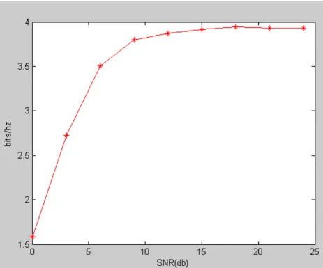
Fig. 3.1 (a) shows a typical simulation. The capacity is saturates at high SNR

because of the modulation scheme. Two antennas transmit independent signals, so the

maximum capacity of this scheme is 4 bits/channel use (2*log (4) =4). We show 2X1 ₂

16

Fig. 3.1 (a) 2X2 MIMO, 4-QAM Modulation, 3 bit Quantizer

Fig. 3.1 (b) 2X1 and 2X2 MIMO, 4-QAM Modulation, 3 bit Quantizer

17

3.2 The maximum information rate about the

discrete-input and discrete-output MIMO

channel

Quantizing the signal at the receiver causes of the loss of information rate. If we

transmit two independent 4-QAM signals at two antennas, and we can distinguish 16

(4*4=16) different signal vectors (which has two elements, and each element is

4-QAM signal), then the information rate is 4 bits/channel use. If we quantize the

receive signals by quantizers, we may not distinguish the all difference at the receiver

and get the maximum information rate. To explain this, we show all combination of

two antenna and modulation signal (here we use a special 4-QAM signal, which real

part is -1 and 5, and imagery part is -5 and 1) in Fig 3.2. We generate a channel

randomly, then all the possible transmit signal vectors pass the channel and are

quantized at the receiver, which was shown in Fig 3.3. In Fig 3.3, we can only

distinguish 12 different signal vectors at the receiver, so the maximum information

rate is 3.58 bit/channel use (log (12)₂ =3.58). We run the algorithm, and show the simulation result in Fig 3.4, in which we see that the channel capacity does not exceed

18

Fig. 3.2 All possible transmit signal vectors in 2X2 quantized MIMO system.

19

20

3.3 Optimal input vector distribution for different

input power constraint

In this section, we analyze the optimal input vector distribution with different

input power constraint in discrete-input and discrete-output MIMO Raleigh flat fading

channel. In our simulation, in order to observe the relationship between the power

constraint and optimal input distribution, we use a special 4-QAM signal (which is the

same in section 3.1). We analyze the optimal distribution with low power constraint in

3.3.1, and analysis high power constraint in 3.3.2.

3.3.1 Low power constraint

In this section, we analyze the optimal input vector distributions with low power

constraint. We constrain the average input power 25 and show all possible transmit

vector in Fig 3.5(a), and these transmit vectors pass a special channel is shown in Fig

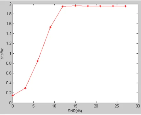
3.5(b). In Fig 3.5(b), we see that we can only distinguish 4 different vectors (we circle

in different color), so the maximum information rate is 2 bits/channel use

(log (4)₂ = ). We run the algorithm and show the simulation result in Fig 3.5(c). In 2 3.5(c), we see that the channel capacity is saturate at 2 bits/channel use. This result

conforms to our anticipation. We show the optimal input vector distribution in high

SNR in Fig 3.5(d). We analyze these distributions as follows.

In Fig 3.5(b), we see that we can only distinguish 4 different signal vectors,

21

(4.5+1.5j,4.5+1.5j).

When we receive the vector (-1.5-4.5j,-1.5-4.5j), the transmit vector may be one

of the three vectors (vector1 (-1-5j,-1-5j), vector2 (-1-5j,-1+j), vector5 (-1+j,-1-5j)).

We summarize the relationship between the output vector and its possible input

vectors in Table 3.1. From this table, we see that we receive the vector

(-1.5+1.5j,-1.5+1.5j) only when vector6 is transmitted, and vector6 has the lowest

power 4(12+ + + = ), so that we see the probability of vector6 is the most in 12 12 12 4 Fig 3.5(d). The three vectors (which are vector1, vector2 and vector5) are transmitted,

then we can receive the vector (-1.5-4.5j,-1.5-4.5j), but the vector2 and vector5 have

the equal power 28, smaller than the power 52 of vector1, so that we see the

probability of vector2 and vector5 are equal, and bigger than vector1. We can analysis

the other distribution in Fig 3.5(b) by the same method. Fig 3.6 shows typical optimal

22 (a)

23 (c)

(d)

24

25

Output vector Possible input vectors

(-1.5-4.5j,-1.5-4.5j) vector1(-1-5j,-1-5j),vector2(-1-5j,-1+j), vector5(-1+j,-1-5j) (4.5-1.5j,4.5-1.5j) vector3(-1-5j,5-5j),vector4(-1-5j,5+1j), vector7(-1+1j,5-5j),vector9(5-5j,-1-5j), vector10(5-5j,-1+1j),vector11(5-5j,5-5j), vector12(5-5j,5+1j),vector13(5+1j,-1-5j), vector15 (5+1j,5-5j). (-1.5+1.5j,-1.5+1.5j) vector6(-1+1j,-1+1j) (4.5+1.5j,4.5+1.5j) Vector8(-1+1j,5+1j),vector14(5+1j,-1+1j), Vector16(5+1j,5+1j)

26

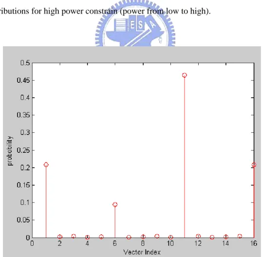
3.3.2 High power constraint

In this section, we constrain the input average power 70 (high input power

constraint), and the other settings are the same with section 3.3.1. We run the

algorithm and show the optimal input vectors distributions in Fig 3.6. When we

transmit one of the three vectors (which are vector8, vector14 and vector16), we can

receive the vector (4.5+1.5j,4.5+1.5j). The vector16 has the most power of the three

vectors, so we see that the probability of vector16 is the most. We can analysis the

other distribution in Fig 3.7 by the same method. Fig. 3.8 shows typical optimal

distributions for high power constrain (power from low to high).

27

28

3.4 AGC to achieve the channel capacity

In our simulation, we discover that when we fix the antenna and modulation

scheme, the AGC dominate the channel capacity. We show the different AGC in Fig.

3.9 and we can tune the AGC until achieve the maximum information rate.

29

(b) From -3 to 3

30

Chapter 4

Simple Relay Case

4.1 Introduction

Now, we want to use our algorithm to study cooperative communication and we

only consider simple cases. We start with the elementary relay channel model as

shown in Fig. 4.1, in which a single relay R assists the communication between the

source S and the destination D. There is no direct link between the source and the

destination.

Fig. 4.1 Elementary Relay Channel

Let the transmit power at the source and the relay be p and p respectively. _R

At both the relay and the destination, the receive symbol is corrupted by additive

white Gaussian noise of unit power. Relay R observes r, a noisy version of transmitted

symbol x. Based on the observation r, the relay transmits a symbol f(r) which is

received at the destination along with its noise n . The relay function f satisfies the ₂

average power constrain (E f r[ ( ) ]2 =P_R).

r = x +n (4.1) ₁

31

4.2 Basic Memoryless Forwarding Strategies

In this section, we introduce two basic memoryless forwarding strategies. We

introduce demodulate forward in 4.2.1 and amplify forward in 4.2.2.

4.2.1 Demodulate And Forward

In DF protocol, demodulation of the received symbol at the relay is followed by

modulation, the relay function for DF can be expressed as

( ) ( )

DF R

f r = P sign r (4.3) where sign(r) outputs the sign of r. Due to the demodulation process, the relay

transmitted symbol does not provide any soft information to the destination.

4.2.2 Amplify And Forward

An AF relay simply forwards the received signal r after satisfying its power constraint.

The relay function for AF can be written as

( ) 1 R AF P f r r P = + (4.4)

Evidently, with AF, the relay tries to provide soft information to the destination. A

disadvantage with this technique is that significant power is expended at the relay

32

4.3 Simulation Results

In this section, we consider simple relay case and Rayleigh flat-fading channel,

and then run our algorithm. We set the total power (source and relay) S, and noise

power N (SNR=S/N). Fig. 4.2 shows in Rayleigh flat-fading channel, more parallel

relay get the better performance. Fig 4.3 shows one relay and no relay, the

performance is similar, and two parallel relay is better. We compare two kind of

different relay strategies we describe in section 4.2, and show the simulation results in

Fig. 4.4, in which, we can see that DF get better performance in high SNR, because in

high SNR relay demodulate received signals more correct. In Fig. 4.5, we show one

relay and different received antenna simulation results, we can see that two received

antennas get better performance. In relay systems, we can trade off number of relays,

and quantization levels, and number of antennas. We show different relays and

quantization levels in Fig. 4.6, in which we see that increase one antenna, get better

performance than increase one-bit quantization. To achieve a specific performance,

we can combination different relays, antennas and quantization levels. We show

33 Fig. 4.2 Different Parallel Relay

34

Fig. 4.4 Different Relay Strategies

35 Fig. 4.6 Different Combination

36 Bibliography

[1] C. Shannon, “A mathematical theory of communication”, Bell Syst. 1984. [2] S. Arimoto, “An algorithm for computing the capacity of arbitrary discrete

memoryless channels”, 1972.

[3] R. E. Blahut , “Computation of channel capacity and rate distortion functions”, 1972.

[4] N. Varnica, X. Ma, and A. Kavcic, ”Capacity of power constrained memoryless AWGN channels with fixed input constellations”,November 2001.

[5] J. Bellorado, S. Ghassemzadeh, and A. Kavcic,”Approaching the capacity of the MIMO Rayleigh flat-fading channel with QAM constellation, independent across antennas and dimensions”.

[6] Obianuju Ndili and Tokunbo Ogunfunmi, “Achieving Maximum possible Speed on Constrained Block Transmission System”.

[7] Josef A.Nossek and Michel T.Ivrlac, ”Capacity and Coding for Quantized MIMO Systems”,2006.

37

About the Author

姓

名：黃俞榮

Yu-Rong Huang

出

生

地：高雄市

出生日期：

1983. 11. 21

學

歷：

1990. 9 ~ 1996. 6

高雄市四維國小

1996. 9 ~ 1999. 6

高雄市私立復華中學

1999. 9 ~ 2002. 6

高雄市立中正高中

2002. 9 ~ 2006. 6

大同大學

電機工程學系

學士