政府公債佔GDP的最適比率 - 政大學術集成

全文

(1)國立政治大學社會科學院經濟學系碩士論文 Department of Economics College of Social Sciences National Chengchi University Master Thesis. 政治大. 政府公債佔 GDP 的最適比率. 立. The Optimal Ratio of Public Debt to GDP. ‧. ‧ 國. 學 y. sit. io. Lin, Ming-Feng. n. al. Ch. engchi. er. Nat. 林銘峰. i Un. v. 指導教授：黃俞寧博士 Advisor: Hwang, Yu-Ning, Ph.D.. 中華民國一百年七月 July, 2011.

(2) 謝辭依稀記得兩年前剛進入經研所時，一開始不太能適應，覺得怎麼跟大學部學的有一段差距，也才讓我了解到經濟這門學科的深度，但好加在，一路上並不孤單，有一大群朋友互相扶持著。首先，我必須感謝我的指導教授黃俞寧老師，老師總是在百忙之中還要耐心的教導我們四位學生，不只是課業上，在生活上也學到很多做人處事的道理。感謝口試委員張瑞娟教授、張淑華教授，兩位老師耐心將本文閱畢，並且給予本文許多建議，使本文更加完整。另外，我要感謝我家人，感謝父母親對我的照顧，讓我沒有負擔的做自己想做的事。感謝我兩位姊姊，總是把我當小孩一樣疼愛，. 治政讓我覺得遇到挫折時總是有依靠。還要感謝在政大遇到的一群禽獸好友們，羅大立賓、小潘潘、布萊迪、翔哥，跟你們混在一起的時間，總是有講不停的垃圾話、 ‧ 國. 學. 看不完的正妹、吃不停的燒烤，賭不停的大老二，雖然似乎都不是什麼正面的活. ‧. 動，但卻豐富了我人生的色彩，認識你們真的是很開心的事情。還要感謝與我相. sit. y. Nat. 同指導教授的其他同學，詩閔、翰屏與柏勳總是在論文遇到瓶頸時，我們會互相. io. er. 加油打氣，讓我並不孤單。當然還有班上曾經幫助過我的人，不管是大事或小事，都很感謝你們。還有很多曾經幫助過我，而我沒有提到的人，我絕對會銘記在心，. al. n. iv n C 謝謝你們。最後，我想要謝謝我生命中最重要的比比，我能夠有今天，全部都是 hengchi U 妳給我的，和妳在一起的時光，是我人生中最美好的時刻，雖然我做出讓你失望難過的事情，自己也相當懊悔，但我不敢奢求你原諒，只希望你把我們在一起快樂的時光放在心裡，我會永遠記得我所犯下的錯，讓我失去了生命中最重要的人，而妳，我會永遠擺在心裡。僅將此論文獻給我的家人、朋友們，因為有你們，才讓我覺得並不孤單。林銘峰僅致於國立政治大學經濟系中華民國 100 年 7 月. I.

(3) 中文摘要. 本文研究目的是在動態隨機一般均衡模型當中，討論政府公債佔國內生產毛額的最適比率。本文建立一封閉經濟體系，討論政府公債佔國內生產毛額的比率改變時，對主要的經濟變數有何影響。不同於先前的研究，我們假設在極大化福利的前提下，找尋最適的政府公債佔國內生產毛額比率。靜止均衡的分析發現，政府公債佔國內生產毛額的比率與消費呈現正向變動的關係，與產出和勞動有著負向變動的關係。除此之外，當政府公債佔國內生產毛額的比率增加時，福利水. 政治大. 準會越來越低，因此，最適的公債比率為零。. 學. ‧ 國. 立. 關鍵字： DSGE、政府公債、國內生產毛額. ‧. n. er. io. sit. y. Nat. al. Ch. engchi. II. i Un. v.

(4) Abstract. The objective of this paper is to investigate the optimal ratio of public debt to GDP by using a micro-based dynamic stochastic general equilibrium (DSGE) model. In this paper, the model that we build is a closed economy. We discuss the effect of the optimal public debt to GDP ratio on primary variables. Different from previous research, we look for the optimal ratio of public debt to GDP that will maximize welfare. In the steady state analysis, we find that the ratio of public debt to GDP has the positive effect on consumption and negative effect on output and labor.. 治政 Furthermore, the welfare level is lowered with the rise 大 in the debt ratios to GDP. Thus, 立 the optimal debt ratio should be 0. ‧ 國. 學 ‧. Keywords: DSGE, public debt, GDP. n. er. io. sit. y. Nat. al. Ch. engchi. III. i Un. v.

(5) Contents 1. Introduction…………………………………………………………………………1 1.1 Motivation………………………………………………………………………1 1.2 Literature review………………………………………………………………..3 2. The model…………………………………………………………………………...5 2.1 Household……………………………………………………………………….5 2.2 Firms…………………………………………………………………………….7 2.2.1 Final goods………………………………………………………………..7 2.2.2 Intermediate goods………………………………………………………8 2.3 Government………………………………………………………………...….10. 政治大. 2.4 Monetary policy…………………………………………………………….....10. 立. 2.5 Market clearing conditions……………………………………….…………....11. ‧ 國. 學. 2.6 Exogenous variables………………………………………………………...…11 3. Steady state…………………………………………………………………...……11. ‧. 3.1 The steady state solution………………………………………………………11 3.2 Parameters and calibration…………………………………………………....13. Nat. sit. y. 3.3 Steady state analysis………………………………………………………...…14. io. er. 3.4 Long run effect of debt ratio……………………………………………..…….15 3.5 Dynamic…………………………………………………………………….....18. n. al. Ch. i Un. v. 3.5.1 Productivity shock ………………………………………………...…….18. engchi. 3.5.2 Government expenditure shock……………………………….…………19 3.5.3 Welfare analysis………………………………………………….………19 4. Conclusion………………………………………………………………………....21 Reference……………………………………………………………………………..22 Appendix1: Optimal price setting………………………………………...………….24 Appendix2: The analytical solution on steady state….……………………...……….25 Appendix3: The graph of shocks…………………..…………………………..……..27. IV.

(6) 1. Introduction. 1.1. Motivation The government debt is an important issue in fiscal policy. In this paper we discuss the optimal ratio of public debt over GDP with a dynamic stochastic general equilibrium (DSGE) model. In 2008, the U.S. subprime mortgage crisis broke out, making the global economic recession. The governments all over the world take expansionary fiscal policy and monetary policy. This behavior not only increases the financial burden on the government, but also increase instability factor for the global economic recovery.. 立. 政治大. In 2010, economic revitalization policy and expansionary monetary policy. ‧ 國. 學. improved economic indicators substantially in the world, but the consequence of. ‧. expansionary fiscal policy also came out.. sit. y. Nat. First, Greece, the overall fiscal deficit to GDP ratio rose sharply to 13 percent in. io. er. early 2010, much higher than the Maastricht Treaty specification standard. Dalamagas. al. (2000) suggests that an increase in the government size has adverse effects on the. n. iv n C economic growth, mainly due to the importance of debt accumulation as a h eincreased ngchi U mean of financing government activities.. Then the market began to review the situation of budget deficit in the euro zone. However, the result is disappointing, the deficit to GDP ratio rose to 11.2 percent in Ireland and 14.3 percent in Spain. Although the proportion does not exceed 10 percent in Italy and Portugal, the ratio of debt to GDP as high as 115.8 percent and 76.8 percent, implying the level of fiscal deficit is very deterioration. The EU debt crisis had caused threat to both the Europe and the global economy. The crisis developed concerning some European country, including European Union members Greece, Ireland, Portugal, and Spain. In the euro zone, member countries 1.

(7) cannot exceed their deficit to 3 percent of GDP. But among the sixteen member countries, thirteen countries have already been warned for excessive deficit. Deterioration of fiscal deficits causes market panic in Europe, the market began to sell bonds issued by these countries. Bonds yield to maturity and the credit default swaps (CDS) price rose sharply. Although the EU proposes 750 billion relief programs, the investors are still worried about the future. The deficit reduction program will affect economic recovery in the euro area, even leading to the global economic recession. On the other hand, the current (2010) ratio of debt to GDP is about 70 percent in. 治政大of another crisis. Smyth and the US. This has raised high concerns over the possibility 立 Hsing (1995) show that economic growth and its determinants, including the debt ‧ 國. 學. ratio are cointegrated and have a long-run stable relationship in the US. Results also. ‧. indicate that the optimal debt ratio is 38.4 percent for debt held by the public and 48.9. sit. y. Nat. percent for total debt.. io. er. The Taiwanese government, which has used the public debt to finance the fiscal. al. deficit in the past ten years, should also be cautious about this issue. In the literature. n. iv n C of Taiwan about public debt, Chenh (2000) show that U e n g c h i government uses the public debt to finance budget deficit after 1980, and thus produced inflation pressure with the high debt accumulates. In the long run, interest rate and trade balance result in the negative effect. Tseng (2002) examines that the government chooses different fiscal policy under tax smoothing hypothesis. His results indicate that the government facing permanent spending should use tax financing while temporary expenditure should use debt to finance. Therefore, how to manage the issuance of debt is an important issue for the fiscal authority, and the ratio of debt to GDP can be an important indicator. It is a top priority in the world. Smyth and Hsing (1995) have examined whether there is an 2.

(8) optimal debt ratio that will maximize economic growth. However, the model lacks the microfundation in the analysis. After, Devereux (2010) base on the framework of dynamic stochastic general equilibrium model to discuss the role of government debt and deficits, and the discussions focus on the choice of government policy. In this paper, by using DSGE model, we follow Devereux (2010) to examine the effect of the optimal public debt to GDP ratio. Different from Smyth and Hsing (1995), we look for the optimal ratio of public debt to GDP that will maximize welfare.. 1.2. Literature review. 立. 政治大. Recently, more and more authors are aware of the importance of public debt and. ‧ 國. 學. budget deficit issue in the world. Now, we review the literature of the public debt,. ‧. which is initiated by Barro and Grossman (1971). They show that government. sit. y. Nat. spending finance by issuing public debt can create multiplier effects. The research. io. al. short run, and neglects the problem of generation burden.. er. means that the net wealth is increased by issuing debt. But the analysis is based on. n. iv n C Friedman’s (1957) developing Income Hypothesis and Ando h ePermanent ngchi U. and. Modigliani’s (1963) developing Life Cycle Hypothesis indicate that the public maximize the lifetime utility and public debt finance generates wealth effect in the limited life. Differing from the view above, Barro (1974) indicates that the altruism behavior exists between parent and children under infinite life cycle, the bequests grant to their children, thus the net wealth effect were failure. He interprets public debt finance concept under Ricardian equivalence theorem and creates an inter-temporal model under rational expectations. The result suggests a forward-looking consumer will internalize the government budget constraint and thus the timing of any tax change 3.

(9) does not affect their spending. The conclusion is also called Barro-Ricardian equivalence theorem. Mundell (1971) claims against the Ricardian equivalence theorem, he indicates the personal borrowing interest rate is higher than the government borrowing interest rate when the capital market is imperfect competition. The government lowers the price of bonds to encourage the individual to hold by raising interest rate, but it generates crowding out effect on consumption and investment. Feldstein (1985) suggests that increasing tax is a more efficient policy than issuing bonds under the different situation. If the interest rate of bond is higher than discount rate, then the. 治政 higher excess burden results from the debt finance. 大立 Bohn (1998) researches the relationship among government deficits, expenditure ‧ 國. 學. and tax rate in the US. Using the data from 1792 to 1988, he finds the deficit which is. ‧. caused by reducing 50 percent to 65 percent tax rate and increasing 65 percent to 70. sit. y. Nat. percent government expenditure can be eliminated by the policy of reducing the. io. er. government expenditure in the future. The remaining part can be eliminated by. al. increasing tax. In other words, if the private sector expects the tax to increase and the. n. iv n C government balances the budget byhdecreasing the expenditure, the wealth effect still engchi U exists to individuals. Smyth and Hsing (1995) extend the work of Barro (1979), and examine whether there is an optimal debt ratio that will maximize economic growth. The growth rate of real GDP is specified as a function of the debt ratio, the debt ratio squared, the growth rates of labor employment, capital services, money stock, and a trend variable. The sample ranges from 1960 to 1991. Hypothesis tests show that economic growth and its determinants, includes that the debt ratio is cointegrated and has a long-run stable relationship. The results also indicate that the optimal debt ratio is 38.4 percent for debt held by the public and 48.9 percent for total debt. 4.

(10) Dalamagas (2000) investigates the relationship between output and government size using time series data on Greece. He suggests that an increase in government size has a negative effect on economic growth, mainly due to the increasing importance of debt accumulation as a mean of financing government activities. After, Devereux (2010) develops the dynamic stochastic general equilibrium to explain the role of government debt and deficits in a close economy constrained by the zero bound on nominal interest rate. His results show that government spending financed by deficits may be far more expansionary than that financed by increasing tax in such a situation.. 治政大 2, we describe the model The rest of this paper is organized as follow. In Section 立 specification, first-order conditions and monetary policy. Next, in Section 3, we solve ‧ 國. 學. the steady state solutions, discuss the steady state calibration and analyze the result of. ‧. the steady state. Moreover, we discuss the effects of the ratio of public debt to GDP in. sit. n. al. er. io. 2. The Model. y. Nat. the short run and long run. Section 4 concludes.. Ch. engchi. i Un. v. 2.1. Household A typical close economy is inhabited by a representative household who seeks to maximize:   C 1-1 Lt 1 G 1 2  t   t  t   t  1 2  t 0  1-  1 1 . (1). where  is discount factor. Here we define Ct as the consumption and Lt as labor supply in time t.  1 is the inverse of the elasticity of inter-temporal substitution,.  is elasticity of labor supply. Household also derive utility from aggregate government spending, denoted by Gt , and  is a parameter capturing the relative 5.

(11) valuation of public consumption in households’ utility function.  2 is the elasticity of public consumption. We assume that the composite consumption good represented by Ct is differentiated across a continuum of individual goods by the CES function, so that Ct is: .  1  1   1  Ct    Ct (i) di   i 0 . (2). Notice that parameter   1 denotes the elasticity of substitution across individual brands. We focus on a model without capital, household have only one form of saving. 治政大time t is: instrument, government bonds. The budget constraint in 立 ‧ 國. 學. PC t t 1   c ,t   Bt 1 - (1  rt ) Bt  M t - M t -1  Wt Lt 1   L ,t    t. (3). Here Bt 1 represents the nominal bond, and  c ,t , L ,t represent the consumption and. ‧. labor income tax. Nominal wage in terms of the composite consumption good are. y. Nat. 1 1 Pt    Pt (i )1 di  is the consumer prices index.  i 0 . n. al. Ch. engchi. er. io. 1. sit. denoted Wt . Profits from firms are represented by  t , rt is nominal interest rate.. i Un. v. In addition, the household must choose individual brands to minimize expenditure conditional on a given composite consumption. The familiar condition for the optimal brand choice is given by:.  P i  Ct i    t  Ct  Pt  . (4). Maximizing utility subject to the budget constraint, household’s optimal behavior implies the following conditions:.  C   P   1  Et  t 1   t     Ct   Pt 1   1  rt 6. (5).

(12) Ct 1 Lt . Wt 1   L,t  Pt 1+ c,t . (6). Eq. (5) is the consumptive Euler equation, it represents the household sector inter-temporal consumption behavior. Eq. (6) represents the tradeoff between consumption and labor.. 2.2. Firms Production is split a competitive final goods sector and a monopolistically competitive intermediate goods sector. There is collection of monopolistically. 治政大output to a competitive sector competitive intermediate goods producers that sell their 立 that produces final output. ‧ 國. 學 ‧. 2.2.1 Final Goods. sit. y. Nat. The final goods are a CES aggregate of intermediate goods. There is a continuum. io. n. al. .  1  1  1  Yt    Yt  i     0 . Ch. engchi. er. of intermediate good indexed by i over the unit interval:. i Un. v. (7). where   1 is a parameter denoting the elasticity of substitution between types of differentiated intermediate goods. The final good firm sells its output at a nominal price Pt and chooses Yt and Yt  i  for all i   0,1 to maximize its profits, given by: PY t t   Pt  i  Yt  i di 1. 0. (8). subject to Eq.(7) in each period. The first-order conditions for this problem are the constraint and:. 7.

(13) .  P i   Yt  i    t  Yt  Pt . (9). Equation (9) expresses the conditional demand for intermediate good i as a decreasing function of its relative price and increasing function of total output. The exact price index for final output is given by: 1. 1 1 Pt    Pt (i )1 di   0 . 2.2.2 Intermediate Goods. (10). 治政大 in order to hire labor and capital. Intermediate goods firms. 立. produce their. 學. Yt i   At Lt i . 1. (11). Lt i  is firm i’s composite employment. We abstract from capital. ‧. where. ‧ 國. individual brands, using the production function:. Nat. sit. y. accumulation, but allow for the presence of a fixed factor of production, so that. n. al. er. io. capital share is set 0    1 . At is a productivity term, common to all firms.. i Un. v. Intermediate firms are monopolistically competitive, and face an elasticity of demand. Ch. engchi. given by   1 in each period. Firms adjust their prices according to the usual Calvo assumption of a constant probability of price change, 1   , however long ago the previous price change was made. Intermediate firms are price takers in factor markets. The market structure requires them to produce as much output as is demanded at a given price. Firms face cost minimization problem, the marginal cost is then: Wt L MCt  1    At. (12). When they adjust their price, firms maximize discounted expected profits, where per. 8.

(14) period profits for each firm i are t  i   Pt  i  Yt  i   Wt Lt  i  . Thus, firm i’s expected discounted profit is written as: 1   1  Wt  j  i   Yt  j  i     j  Pt  i  Yt  j  i  t  i   Et   t  j       Pt  j Pt  j  At  j   j 0   . where  t  j.  Ct  j     Ct . (13). . represent the ratio of marginal utility between period t  j. and period t , Wt  wt Pt is the aggregate nominal wage, and the demand function .  P i   for firm i’s good is Yt  j  i    t  Yt  j .  Pt  j . 立. The profit maximizing price for firm i , 政治大. . Et   t  j   Pt  j 1  MCt  jYt  j. .   1. j. j 0. . Et   t  j   Pt  j j. 1 . j 0. Yt  j. (14). Nat. y. ‧. Pt , f  i  . 學. ‧ 國. setting its price at time t is then:. io. sit. However, the price index Pt is determined by the familiar Calvo (1983) staggered. n. al. er. price system, with each firm given a subsidy to eliminate the effect of a price mark-up.. Ch. i Un. v. The pricing system can be written in a recursive framework with two auxiliary variables,. engchi. A1t and A2t , in the following way:. A1t  MCt Pt 1 Yt  t 1 A1t 1. (15). A2t  Pt 1 Yt   t 1 A2t 1. (16). Pt , f  i  . . A1t   1 A2t. (17) 1. Pt  1    Pt , f 1   Pt 11  1. (18). The weight  in the aggregate price equation represents the fraction of prices which are expected to remain unchanged, in other words, it stays at last period’s level. 9.

(15) Pt 1 . A fraction 1    of firms are forward-looking with Pt , f determined from maximizing expected profits.. 2.3. Government The fiscal authority receives taxes and borrows to finance government expenditure, issuing money and bonds. Given its source of labor and consumption tax revenues, so that the government budget constraint is as follows:. Gt  Tt  where. 立. Bt  1  rt  Bt 1 Pt. . M t  M t 1 Pt. (19). 政治大 Wt Lt Pt. (20). 學. ‧ 國. Tt   c ,t Ct   L ,t. ‧. 2.4. Monetary Policy. y. Nat. Assume that the monetary authority follows an interest rate rule, given by:. sit. n. al. (21). er. io. rt  r rt 1  1  r   r   ( t   )   y yt   . v. where r is the steady-state value of interest rate,  is the monetary authority’s. Ch. engchi. i Un. inflation target, yt represents output deviations from the steady state. The parameter.  r is autocorrelation of interest rate.  represents autocorrelation of inflation target. Autocorrelation of output is represented by  y . We assume that   1 and. y  0 .. 10.

(16) 2.5. Market clearing conditions The model is closed by imposing the following resource constraints and market clearing conditions: At Lt1  Yt  Ct  Gt. (22). 2.6. Exogenous variables The exogenous processes in the model are all assumed to follow first-order autoregressive process:. 政治大. Gt  1  G  G  GGt 1   G , 0  G  1. 立.  G ,  A . 學. ‧ 國. log At  1   A  log A   A log At 1   A , 0   A  1 N  0,  . (23) (24) (25). ‧. where G and A means the steady state value of government spending and. Nat. sit. n. al. er. io. are chosen to be 0.9.. y. productivity. The persistence of the government expenditure and the productivity term. 3. Steady state. Ch. engchi. i Un. v. 3.1. The steady state solution We solve the steady-state solutions in this section. We discuss the optimal ratio of public debt to GDP. Then Eq. (19) can be rewrite as:. Gt  Tt  bbYt  1  r  bbYt 1  . M t  M t 1 Pt. (26). The variable bb represents the ratio of public debt to GDP. We assume the ratio is a constant in each period. To simplicity, we assume that the productivity and price level are equal to one. Then 11.

(17) Eq. (11), Eq. (14) and Eq. (12) can be stated as:. Y  L1. (27).  1    1   W   1    L    MC . (28) (29). Moreover, the relative valuation of public consumption and money supply on steady state are also equal to one. Therefore, Eq. (5)-(21) can be degenerated to eight equations for eight endogenous variables L, Y , C, G, MC, T ,W , r . The steady state solutions can be represented as below.. 政治大. First, Eq. (5) on the steady state can be represented:. . 1 1 r. (30). 學. ‧ 國. 立 Then Eq. (6) can be states as:. ‧ y. (31). sit. Nat.    11   1   L   C      1   c  L . 1. 1. io. al. n. represented by:. er. The rewritten government budget constraint Eq. (26) on the steady state can be. ni GCh T  rbbY U engchi. v. T   cC   LWL. (32) (33). Next, combining Eq. (31) - Eq. (33) and the market clearing condition Eq. (22) can be stated as: 1.    11    1   L   L1    G   1   c     L 1. So, we get the steady state value of labor:. 12. (34).

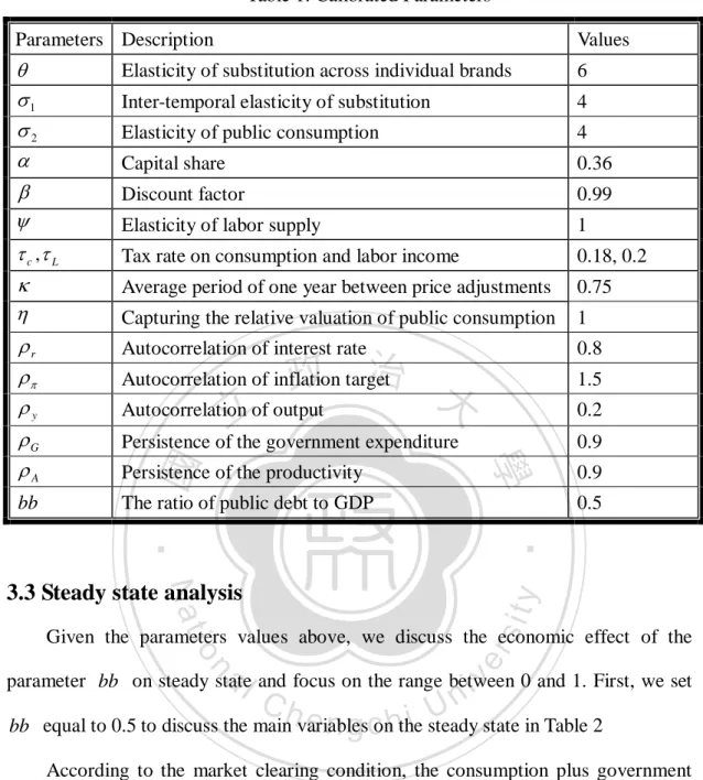
(18) 1. 1  1 1     1 1   1       1 L  1 1      c      ss L     11      1  rbb   L      . 1 1        . (35). Finally, we obtain eight Eqs. (27)-(34) to determine the eight steady state values. L, Y , C, G, MC, T ,W , r .. 3.2. Parameters and Calibration. 政治大 in Table 1. Following Scharler (2006), we set the discount 立. We calibrate the parameters which determine the steady state. All parameter are summarized. factor. price-marginal cost markup factor for goods is set at. .  1.  1.2 (i.e.   6 ). The. ‧. ‧ 國. 學.   0.99 implies a steady state interest rate of about one percent. The steady state. coefficients  and  which determine the inter-temporal elasticity of substitution. y. Nat. sit. and the labor supply elasticity, are set to equal to 4 and 1. The capital share  is set. n. al. er. io. to 0.36.  c  0.18 and  L  0.2 , which means the tax rate on consumption and labor. i Un. v. income. We set   0.75 , consistent with an average period of one year between. Ch. engchi. price adjustments. To capturing the relative valuation of public consumption  is set to 1. Moreover, the monetary policy rule is calibrated to the estimates in Clarida et al. (2000), so r  0.8 ,   1.5 , and  y  0.2 . Finally, we set the ratio of debt to GDP bb  0.5 to match the facts of the US.. 13.

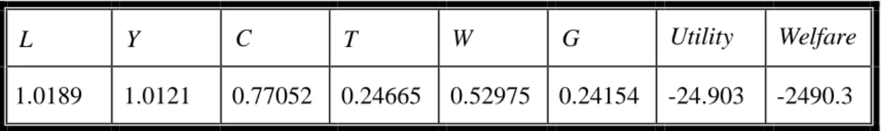
(19) Table 1: Calibrated Parameters Parameters Description. Values.  1 2 . Elasticity of substitution across individual brands. 6. Inter-temporal elasticity of substitution. 4. Elasticity of public consumption. 4. Capital share. 0.36.  . Discount factor. 0.99. Elasticity of labor supply. 1.  c , L  . Tax rate on consumption and labor income. 0.18, 0.2. Average period of one year between price adjustments. 0.75. Capturing the relative valuation of public consumption. 1. r  y. Autocorrelation of interest rate. 0.8. Autocorrelation of inflation target. 1.5. G A. Persistence of the government expenditure. 0.2 0.9. ‧ 國. 學. bb. 政治大 Autocorrelation of output 立 Persistence of the productivity The ratio of public debt to GDP. 0.9 0.5. ‧. Nat. sit. y. 3.3 Steady state analysis. n. al. er. io. Given the parameters values above, we discuss the economic effect of the. i Un. v. parameter bb on steady state and focus on the range between 0 and 1. First, we set. Ch. engchi. bb equal to 0.5 to discuss the main variables on the steady state in Table 2. According to the market clearing condition, the consumption plus government expenditure are equal to output level. The capital share is 0.3, in other words, the labor share is equal to 0.7. According to the production function above, the labor to the power of 0.7 are equal to output level. On the other hand, the tax are not equal to government expenditure are caused by bond issuing. The government expenditure must include the interest payments on bond, so the government consumption plus the interest payments on bond should equal to the tax level.. 14.

(20) Table 2: Primary variables in steady state values when bb  0.5 . L. Y. C. T. W. G. Utility. Welfare. 1.0189. 1.0121. 0.77052. 0.24665. 0.52975. 0.24154. -24.903. -2490.3. 3.4. Long run effect of the debt ratio Now, we discuss the effect of bb on the steady state. The analytical solutions for output and consumption in the steady state can be stated as below:. 治政        11   1    1   大      立      1. L. 1. 1. c.    11    1  rbb  L . 1.    . (36). 學.    . ‧. ‧ 國.  1      11   1   L   1 1   11   c         1  1     1  rbb  L   . io.    11   1   L   1 C ss     1   c   . n. al. Ch. sit. Nat. 1. y. 1. er. Y ss. 1. 1 1  1 1   . engchi. i Un. v.       .    1 1   . (37). We find bb has the negative effect on output and positive effect on consumption. It means higher the ratio of public debt to GDP caused the output to decrease. The results are similar to the Euro debt crisis. The countries which hold a large amount of debt, in order to repay the interest on public debt, will have to issue more bonds for repayment. Moreover, the increase in the ratio of public debt to GDP will cause the consumption to increase. Furthermore, the analytical tax and government spending solution on the steady state can be represented by:. 15.

(21) 1.    11   1   L   1 ss T    1   c   . 1  1 1     1 1   1       1 L  1 1      c          11     1  rbb  L   . 1  1 1     1 1   1       1 L  1 1       c     11        L     11      1  rbb  L   .       .   . 1 1        .  1 1   1 1   . (38).   . 1  1 1   1     1 1   1        L 1    1   c     1  1   c     11   1   L       G ss   c      L   11     1   c      1  rbb      . 立. 政治大. ‧ 國. 學.        11   1   L   1 1       c   1   c    L   11           rbb       11        1  rbb  L      1.  1 1   1 1   . (39). ‧. n. er. io. sit. y. Nat. al. Ch. engchi. i Un. v. The first term of taxes is consumption tax and the second term is the labor income tax. The effect of bb on consumption tax in the steady state is positive effect, but the income labor tax is negative effect. In the steady state, the taxes are equal to government spending plus the interest of public debt. We rewrite the form of government budget constraint to discuss the ratio of public debt to GDP. According to the Eq. (32), the government spending in the steady state is mainly affected by taxes and output, but Eq. (39) is difficult to see the effect on bb .. 16.

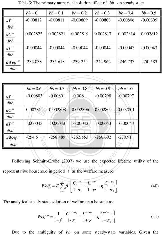
(22) Table 3: The primary numerical solution effect of bb on steady state bb  0. bb  0.1. bb  0.2. bb  0.3. bb  0.4. bb  0.5. ss. dY dbb. -0.00812. -0.00811. -0.00809. -0.00808. -0.00806. -0.00805. dC ss dbb. 0.002823. 0.002821. 0.002819. 0.002817. 0.002814. 0.002812. dT ss dbb. -0.00044. -0.00044. -0.00044. -0.00044. -0.00043. -0.00043. dWelf ss dbb. -232.038. -235.613. -239.254. -242.962. -246.737. -250.583. bb  0.6. bb  0.7. dY ss dbb. -0.00803. -0.00801. dC ss dbb. 0.00281. dT ss dbb dWelf ss dbb.  0.9 政bb  0.8治 bb 大. bb  1.0. -0.00798. -0.00797. 0.002808. 0.002806. 0.002804. 0.002801. -0.00043. -0.00043. -0.00043. -0.00043. -0.00043. -254.5. -258.489. -262.553. -266.692. ‧. n. al. er. io. sit. Nat. -270.91. y. ‧ 國. 學. -0.008. 立. i Un. v. Following Schmitt-Grohé (2007) we use the expected lifetime utility of the. Ch. engchi. representative household in period t as the welfare measure:.  Ct 1-1 Lt 1 Gt1 2  Welft  Et       1 2  t 0  1-  1 1  . t. (40). The analytical steady state solution of welfare can be state as: Welf ss . 1  C ss 1-1 Lss 1 G ss1 2       1    1-  1 1  1 2 . (41). Due to the ambiguity of bb on some steady-state variables. Given the parameter values in Table 1, we can obtain the numerical results in Table 3 for bb ranging from 0 to 1. From the table 3, we can see that the relationship between taxes 17.

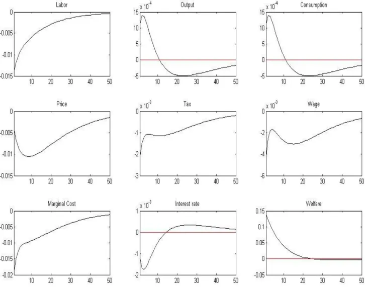
(23) and bb in the steady state is negative. Consequently, the effect of labor income tax is larger than the effect of consumption tax in this range. We know that bb has the negative effect on output and positive effect on consumption. Moreover, we find the influence of bb on the output will decline with bb rises. In other words, the output will decrease less and less when bb rises. Otherwise, its influence on consumption is also lower with bb rises; it means the consumption will increase less and less when bb rises. There is no significant effect on taxes with the different bb values. Furthermore, there is negative relationship between welfare and bb on the steady state. The result means the large debt that government accumulates will lead to greater welfare loss. The influence of bb. 立. bb rises.. ‧ 國. 學. 3.5. Dynamic. 治政 on welfare will increase 大 with. ‧. All parameters values are listed in Table 1. We set the ratio of public debt to GDP. sit. y. Nat. bb  0.5 to match the facts of long term average level on the US. The exogenous. io. al. er. process is assumed to follow first-order autoregressive process, and the persistence of. n. productivity and government expenditure are established 0.9. Both of the standard deviations are set to 0.01.. Ch. engchi. i Un. v. 3.5.1 Productivity Shock Figure 1 shows the impulse response paths following a shock to the productivity in Eq. (23). Both output and consumption rise, while labor falls. The real wage rises more than the increase in the consumption. The result leads to lower taxes. Under the positive productivity shock, the price index fall (marginal cost lowers) and the interest rates fall (consumption rises for larger income). Marginal cost falls due to the positive productivity shock. The welfare rises intuitively.. 18.

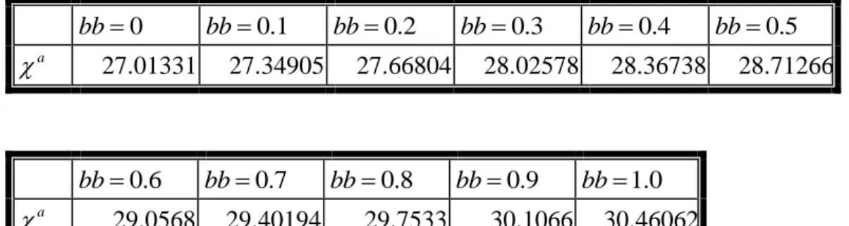
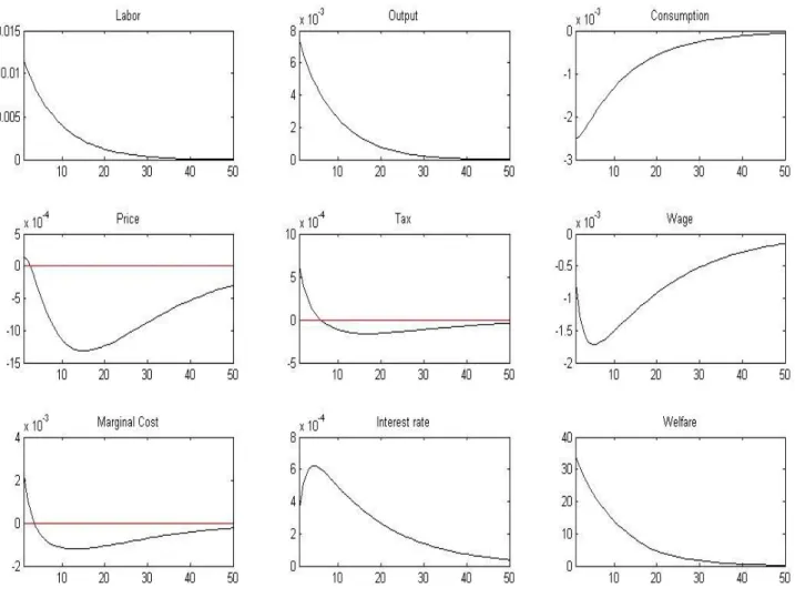
(24) 3.5.2 Government Expenditure Shock Figure 2 shows the impulse response paths for an increase government spending in Eq. (22). The labor and output rise as a result of the expansionary fiscal policy. The labor rise, so that marginal cost of firms rises. The tax rises because the labor income tax rises larger than the decrease in the consumption tax. The consumption fall result from the tradeoff between consumption and labor. The price index rises because of the lower marginal cost. The interest rate rises result from lower consumption. According to the analysis above, the welfare rises consequently.. 3.5.3 Welfare analysis. 立. 政治大. Following Lucas (1987), we evaluate the welfare criterion as a fraction  .. ‧ 國. 學. ‧.     a  ss  1-1 1  C        100   Lss 1 G ss1 2  a t   CV0        1-  1 1  1 2  t 0     . Nat. sit. y. (43). al. er. io. where C ss , Lss and G ss are the steady-state value of consumption, labor and. v. n. public consumption. The fraction  a of steady state consumption that the household. Ch. engchi. i Un. would decrease to be as well off under the steady state as under a regime a . Consequently, a higher value of  a means higher welfare cost. Given the parameter value above, we evaluate the welfare criterion under bb ranging between 0 and 1 as below:. 19.

(25) Table 4: The welfare criterion bb  0. . a. . a. bb  0.1. 27.01331. bb  0.6. bb  0.2. 27.34905. bb  0.7. 29.0568. bb  0.3. 27.66804. bb  0.8. 29.40194. bb  0.4. 28.02578. bb  0.9. 29.7533. 28.36738. bb  0.5. 28.71266. bb  1.0. 30.1066. 30.46062. Table 4 reports the welfare criterion. The ratio of public debt to GDP bb in this range, we find that the variable  a rises continuously. It means that the welfare cost. 政治大 is less 立than 0.5. If the value of bb. continuously rises. We find that the means of labor and output change irregularly when the value of bb. is more than 0.5, the mean. ‧ 國. 學. of labor and output fall smoothly with the rise in bb . Moreover, the mean of consumption is almost unchanged under different debt ratios to the GDP. The mean of. ‧. government spending falls when the value of bb rises. The results imply that the. Nat. n. al. er. io. sit. y. welfare level is lowered with the rise in bb . Thus, the optimal debt ratio should be 0.. Ch. engchi. 20. i Un. v.

(26) 4. Conclusion In this paper, we investigate the optimal ratio of public debt to GDP by using a micro-based dynamic stochastic general equilibrium (DSGE) model. To construct the general equilibrium model, we discuss the optimal ratio of public debt to GDP. The discussions focus on the effects of the public debt to GDP ratio. We analyze the result of steady state in the short run and long run. In the long run analysis, we find that the ratio of public debt to GDP has the negative effect on output and positive effect on consumption. The results are similar to the Euro debt crisis. The countries which hold large amount of debt, in order to. 治政大 bonds for repayment. The repay the interest on public debt, will have to issue more 立 result shows the large debt that government accumulates will lead the welfare to ‧ 國. 學. decline. On the other hand, we discuss the welfare criterion in the short run. We find. ‧. that the welfare cost rises continuously under the ratio of public debt to GDP ranging. sit. y. Nat. between 0 and 1. In other words, the optimal debt ratio should be 0.. io. er. The debt ratio to the GDP would be an important issue in the future. We. al. conclude this paper by providing some issues for future research. First, the results are. n. iv n C represented under the specificationhof parameter values e n g c h i U and may change for different. parameters. Second, the model that we build is a closed economy. The situation of real world is almost open economy. The discussion neglects some important variables under the specification of model. The result may change for the new variables.. 21.

(27) References Ando A. and Modigliani F. (1963), "The 'Life-Cycle' Hypothesis of Saving: Aggregate Implications and Tests." American Economic Review, 53(1), 55-84. Barro R. J. and Grossman H. I. (1971), "A General Disequilibrium Model of Income and Employment," American Economic Review, 61(1), 82-93. Barro R.J. (1974), "Are Government Bonds Net Wealth?" The Journal of Political Economy, 82(6), 1095-1117. Barro R.J. (1979), "On the Determination of the Public Debt," The Journal of Political Economy, 87(5), 940-971.. 政治大 Bohn H. (1998), "The Behavior 立 of U.S. Public Debt and Deficit," The Quarterly Journal of Economics, 113(3), 949-963.. ‧ 國. 學. Chen Y.Y. (2000), "The Government Budget Deficit and The Macroeconomic Development,". ‧. Master’s thesis, University of Donghwa, Hualien, Taiwan. (in traditional Chinese). Nat. n. al. er. io. sit. y. Dalamages B. (2000), "Public Sector and Economic Growth: The Greek Experience." Applied Economics, 32(3), 277-288.. i Un. v. Devereux M.B. (2010), "Fiscal Deficits, Debt, and Money Policy in Liquidity Trap," Globalization and Monetary Policy Institute Working Paper No. 44.. Ch. engchi. Feldstein M. S. (1985), "The Optimal Level of Social Security Benefits," Quarterly Journal of Economics, 100(2), 303-320. Friedman M. (1957), "A Theoty of The Consumption Function," Princetion, NJ: Princeton University Press. Lucas, R.E. (1987), "Model of Business Cycles," Basil Blackwell, New York. Scharler J. (2006), "Do Bank-Based Financial Systems Reduce Macroeconomic Volatility by Smoothing Interest Rates?" Oesterreichische Nationalbank Working Paper, No.117.. 22.

(28) Schmitt-Grohé , S. and M. Uribe (2007), "Optimal Simple and Implementable Monetary and Fiscal Rules," Journal of Monetary Economics, 54(6), 1702-1725. Smyth D.J. and Hsing Y. (1995), "In Search of An Optimal Debt Ratio for Economic Growth," Contemporary Economic Policy, 13(4), 51-59. Tseng C.C. (2002), "Public Debt and Fiscal Policy – An Empirical Study of Taiwan," Master’s Thesis, University of Taiwan, Taipei, Taiwan. (in traditional Chinese). 立. 政治大. ‧. ‧ 國. 學. n. er. io. sit. y. Nat. al. Ch. engchi. 23. i Un. v.

(29) Appendix 1: Optimal price setting When setting a new price in period t firm seeks to maximize the current value of its dividend stream, conditional on that price being effective: 1   1   W i Y i P i j  t    t j   t j   Max t  i   Et   t  j    Yt  j  i      P Pt  j  At  j  j 0  t  j  . (A1). Subject to the sequence of demand constraints: .  P i   Yt  j  i    t  Yt  j  Pt  j . (A2). 政治大. Here the problem is written as maximizing real profits discounted by the stochastic. 立. discount factor as well as the probability of being able to make price changes.. ‧ 國. 學.  1 Wt  j  i   1 j  Pt  i    Max t  i   Et   t  j    Y  t j  Pt  j  Pt  i   At  j P j 0 t  j     . ‧.  Pt  i      Pt  j . Nat. al. To simplicity: .   1 Pt  i  Et   t  j   j 0. j. Yt  j Pt  j. Ch. sit. .  P i    Et   t  j    MCt  j  t   Pt  j  j 0   . j. engchi. er. j 0.  P i     1  t   Pt  j . n. Et   t  j  . j. io. . 1  1  Yt  j   (A3)     . y. The first order condition for this problem is:. . i Un. . v.  1. Yt  j Pt  j 2. Pt  j 1 Yt  j   Et   t  j   Pt  j 1  MCt  jYt  j j. (A4). (A5). j 0. Finally, we get the flexible price: . Pt , f  i  . .   1. Et   t  j   Pt  j 1  MCt  jYt  j j. j 0. . Et   t  j   Pt  j j. j 0. 24. 1 . Yt  j. (A6).

(30) Appendix 2: The analytical solution on steady state We discuss the effect of bb on the steady state. The influence of mainly variables is represented below: In addition, we define: 1 1  1 1 1   1    r  1          L  c    2 1  rbb   L    .     . 1 1  1 1 1   1    1        1 1     dY ss  L  c   dbb  1 1        1  rbb   L  . (A7).   . 政治大. io. 1 1  1 1 1   1    1        1 dLss  L  c   dbb  1 1        1  rbb   L  . n. al. where  .   11    . Ch. engchi.  2  2 1 1  . 1 1   . (A9). 1   . (A10). y. 1 1      . sit. Nat. 1 1  1     1   L   1 1   c  1  1 dW ss   dbb 1  rbb   L    1 1         .     . ‧. ‧ 國. 1 1  1     1   L   1 1   c  1   1  rbb   L    1 1         . 學.   1   L   1 dC   dbb  1   c   ss. 立      . (A8).  1 1 . er. 1. 1 1      . 1 1      . i Un. v. (A11). , the reasonable range of  should be greater than zero but. less than one. All equations have the same formula  ; therefore, we determine the sing of this formula first. According to the parameter values in Table 1, the formula.  is negative. The sign of other formula is not difficult to see and then we can get the result as below:. dY ss 0 dbb. (A12). dC ss 0 dbb. (A13). 25.

(31) dW ss 0 dbb. (A14). dLss 0 dbb. (A15). The other variable can’t easy to see the sign directly. We must into the parameter values to determine the sign of formula. The influence of other mainly variable can be state as:  dW ss ss dT ss dC ss dLss   c  L  L  W ss  dbb dbb dbb   dbb. (A16).  dG ss dT ss dY ss    r  Y ss  bb  dbb dbb dbb  . 立. 政治大 dC ss  L* dbb.  . . dLss  G* dbb.  . dG ss   dbb . . ‧. ‧ 國.  . . 學. dWelf ss 1  ss  C dbb 1  . (A17). n. er. io. sit. y. Nat. al. Ch. engchi. 26. i Un. v. (A18).

(32) Appendix 3: The graph of shocks. Figure 1: Impulse responses following a shock to productivity. 立. 政治大. ‧. ‧ 國. 學. n. er. io. sit. y. Nat. al. Ch. engchi. 27. i Un. v.

(33) Figure 2: Impulse responses following a shock to government spending. 立. 政治大. ‧. ‧ 國. 學. n. er. io. sit. y. Nat. al. Ch. engchi. 28. i Un. v.

(34)