在硬式即時系統下基於工作量延緩之任務間動態電壓調整演算法

國

立

交

通

大

學

資訊科學與工程研究所

碩

士

論

文

在硬式即時系統下基於工作量延緩之任務間動態

電壓調整演算法

A Deferred-Workload-based Inter-Task Dynamic Voltage Scaling

Algorithm for Hard Real-Time Systems

研 究 生：蔡羽航

指導教授：王國禎 博士

在硬式即時系統下基於工作量延緩之動態電壓調整演算法

A Deferred-Workload-based Inter-Task Dynamic Voltage Algorithm for Hard

Real-Time Systems

研 究 生：蔡羽航 Student：Yu-Hang Tsai

指導教授：王國禎 Advisor：Kuochen Wang

國 立 交 通 大 學

資 訊 科 學 與 工 程 研 究 所

碩 士 論 文

Submitted to Institute of Computer Science and Engineering College of Computer Science

National Chiao Tung University in Partial Fulfillment of the Requirements

for the Degree of Master

in

Computer Science

June 2006

Hsinchu, Taiwan, Republic of China

在硬式即時系統下基於工作量延緩之任務間

動態電壓調整演算法

學生：蔡羽航 指導教授：王國禎 博士

國立交通大學 資訊學院 資訊科學與工程研究所

摘 要

這幾年來，個人數位助理與手機等手持裝置越來越普遍。因為這些裝置是

由電池供電，所以能源節省是一個重要的問題。動態電壓調整策略根據處

理器的工作量動態地調整處理器的頻率及電壓，是一種低耗能的設計技

術。一個動態電壓調整演算法的好壞取決於如何準確地估計寬裕時間

(slack time)。本論文提出一個基於工作量延緩之任務間動態電壓調整演

算法，稱為dwDVS。dwDVS有兩個特色，第一是為每一任務保留一個時間區

間，即使是在最壞的情況下，每一個任務都能夠在此時間區間內執行完它

的工作量。用此種方法，可以有效率地估算從優先權較低的任務中所能夠

利用的寬裕時間；第二是延緩這些被保留的時間區間，使這些時間區間儘

可能靠近其對應任務之截止期限。用此種方法，處理器的頻率即使是在沒

有寬裕時間可利用的情況下也可以調降。模擬結果顯示，相較於Static

[1]、laEDF [1] 及 DRA [2]，dwDVS節省了 40-70%、10-20% 及 3-10% 的

能源消耗，且與最佳理論值Bound至多只有12%的差距。

關鍵詞：基於工作量延緩、硬式即時系統、任務間動態電壓調整、寬裕時

間、實際工作量、最差執行時間。

A Deferred-Workload-based Inter-Task

Dynamic Voltage Scaling Algorithm for Hard

Real-Time Systems

Student: Yu-Hang Tsai Advisor: Dr. Kuochen Wang

Department of Computer Science National Chiao Tung University

Abstract

Hand-held devices such as personal digital assistants (PDAs) and cellular phones are getting more and more popular in recent years. Energy consumption is a critical issue because these devices are battery powered. Dynamic voltage scaling (DVS) is a low-power design technique that adjusts the CPU frequency and voltage levels dynamically based on CPU workloads. The performance of a DVS algorithm largely depends on how to estimate slack time accurately. In this thesis, we propose a deferred-workload-based inter-task DVS algorithm (dwDVS), which has two features. The first is that we reserve a time interval for each task to execute and its workload can be completed in this time interval even in the worst-case condition, which means that the actual workload (execution time) of each task is equal to its worst-case execution time. In this way, we can estimate the slack time from lower priority tasks more aggressively. The second is that we defer these reserved time intervals, which means that a reserved time interval will be shifted to the deadline of its corresponding task as close as possible. In this way, the operating frequency can be reduced even without slack time. Simulation results show that the proposed dwDVS reduces the energy consumption by 40-70%, 10-20%, and 3-10% compared with the static voltage scaling (Static) [1], laEDF [1], and DRA [2] algorithms, respectively, and approaches

theoretical low bound (Bound) by an margin of at most 12%.

Keywords: deferred-workload-based, hard real-time system, inter-task dynamic voltage

Acknowledgements

Many people have helped me with this thesis. I deeply appreciate my thesis advisor, Dr. Kuochen Wang, for his intensive advice and instruction. I would like to thank all the classmates in Mobile Computing and Broadband Networking Laboratory for their invaluable assistance and suggestions. This work was supported by the NCTU EECS-MediaTek Research Center under Grant Q583.

Finally, I thank my Father and Mother for their endless love and support.

Contents

Abstract (in Chinese) i

Abstract (in English) iii

Acknowledgements v

Contents vi

List of Figures viii

List of Tables ix

Chapter 1 ... 1

Introduction ... 1

Chapter 2 ... 3

Related Work ... 3

2.1 Categories of Existing Real-Time Schedulers... 3

2.2 Categories of Existing Slack Time Estimation Strategies ... 3

2.3 Comparison of Existing Inter-Task DVS Algorithms... 5

Proposed Deferred-workload-based DVS (dwDVS)... 8

3.1 System Model ... 8

3.2 Problems of Most Existing Inter-Task DVS Algorithms... 9

3.3 The Basic Idea of dwDVS ... 10

3.4 The Detailed Procedure of dwDVS ... 10

Chapter 4 ... 15

Simulation Results and Discussion... 15

4.1 Classical Inter-Task DVS Algorithms ... 15

4.2 Simulation Model ... 16

4.3 Effect of Worst-Case Utilization on Energy Consumption... 16

4.4 Effect of WCET/BCET Ratio on Energy Consumption ... 17

4.5 Effect of Number of Tasks in a Task Sets on Energy Consumption... 18

Chapter 5 ... 20

Conclusions and Future Work... 20

5.1 Concluding Remarks ... 20

5.2 Future Work ... 20

Bibliography... 22

List of Figures

Fig. 1. An illustration of stretching to NTA... 4

Fig. 2. An illustration of incorrect slack time estimation from T2,1 based on example task set 1... 9

Fig. 3. Determine a reserved time interval for a task instance. ... 13

Fig. 4. An illustration of dwDVS based on example task set 2 ... 14

Fig. 5. Effect of worst-case utilization on energy consumption. ... 17

Fig. 6. Effect of WCET/BCET ratio (actual workload) on energy consumption. .... 18

List of Tables

Table 1. Comparison of existing inter-task DVS algorithms... 7

Table 2. Example task set 1. ... 9

Table 3. Example task set 2. ... 14

Chapter 1

Introduction

Hand-held devices are battery powered for mobility. These devices usually require powerful processors to handle various multimedia applications. The energy consumption

E of a CMOS circuit is given by E =C_eff ⋅V_dd2 ⋅C [3], where is the effective switched capacitance, is the supply voltage, and is the number of execution cycles. It can be seen that the energy consumption has a quadratic dependency on the supply voltage. Therefore, lowering the supply voltage is an effective technique for reducing energy consumption.

eff

C

dd

V C

However, a real-time task might violate its time constraint because lowering the supply voltage implies reducing the maximum achievable CPU frequency and hence increasing the execution time of this task. Therefore, DVS algorithms lower the supply voltage of hand-held devices to the lowest possible level while still guaranteeing all deadlines. That is, the devices only need to satisfy the performance requirements of applications while choosing proper CPU frequencies. In addition, the processors of these devices must support multiple CPU frequency and voltage levels, such as Intel Xcale [4][5] and Transmeta

Cursoe [6].

However, DVS also brings some overheads, such as an increase in number of preemptions, which results in increasing energy consumption in memory subsystems, and extra energy consumption and time for voltage transitions. Fortunately, these overheads are usually small enough so that we assume that they can be neglected [1][7][8][9].

There are two categories of DVS algorithms: z Inter-task DVS [1][2][8][9][10][11]

Inter-task DVS adjusts the CPU frequency task by task. It means that the operating frequency will be set to a proper value when a real-time task is ready to execute and won’t be changed until has already completed or has been preempted.

i

T

i

T

z Intra-task DVS [12][13][14]

Intra-task DVS adjusts the CPU frequency within a task. It means that frequency and voltage transition points will be determined offline. During the execution of a real-time task , if the current time reaches a frequency and voltage transition point, the operating frequency will be set to a proper value and won’t be changed until next frequency and voltage transition point.

i

T

In this thesis, we focus on the inter-task DVS. We propose an inter-task DVS algorithm called dwDVS that estimate the slack time from lower priority tasks more aggressively. As a result, we can have a good performance on reducing energy consumption.

The rest of this thesis is organized as follows. In Chapter 2, we review four existing slack time estimation strategies and several inter-task DVS algorithms. In Chapter 3, we describe the system model of the target hard real-time systems. Then, we depict the basic idea and details of the proposed DVS algorithm. In Chapter 4, simulation results are evaluated and discussed. Finally, we conclude with a summary and future work in Chapter 5.

Chapter 2

Related Work

2.1 Categories of Existing Real-Time Schedulers

Inter-task DVS algorithms usually combine with real-time schedulers. The two most popular real-time schedulers are the Rate-Monotonic (RM) scheduler and

Earliest-Deadline-First (EDF) scheduler [15][15]. The RM scheduler always gives the

highest priority to the task which has the shortest period in the ready queue. The EDF scheduler always gives the highest priority to the task which has the latest deadline in the ready queue.

2.2 Categories of Existing Slack Time Estimation

Strategies

DVS usually exploits slack time to adjust CPU frequency and voltage levels in order to guarantee all deadlines. Therefore, a good slack time estimation method is very important to reduce energy consumption. Existing inter-task DVS algorithms usually exploit one or more of the following four strategies to estimate the slack time [7], and it is possible to modify the original version to improve the performance on reducing energy consumption.

(1). Minimum constant speed

Static voltage scaling [1], DRA [2], lppsRM [10], and lppsEDF [10] used this strategy. This strategy estimates the lowest possible constant CPU frequency under the time constraint that all deadlines must be met. Therefore, it needs to know the worst-case

processor utilization Uworst, which can be computed as follows:

∑

where is the number of tasks in the task set, is the worst-case execution time of a task , and is the period of a task . The operating frequency is set to

, where is the maximum CPU frequency.

n wi i T pi Ti max f U f = _worst× f_max

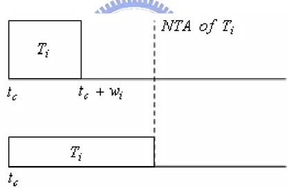
(2). Stretching to NTA (next task arrival time)

ccRM [1], DRA [2], lppsRM [10], and lppsEDF [10] used this strategy. This strategy reduces the operating frequency as shown in Fig. 1. If a task is ready to execute at current time , and the NTA of is later than

i

T

c

t T_i t_c+ , where is the worst-case w_i

execution time of , then can be executed at a lower operating frequency so that will complete at its NTA in the worst-case condition.

i

w

i

T Ti Ti

Fig. 1. An illustration of stretching to NTA.

(3). Priority-based slack stealing

DRA [2], lpSEH [8], and PLG [11] used this strategy. This strategy reduces the operating frequency based on the following scheme. If a higher priority task has been completed before its WCET, it has slack time . The next lower priority task

can exploit the slack time to lower its operating frequency as follows:

i T ) (T_i slack T_j ) (Tj f 4

max ) ( ) ( f T salck w w T f i j j j × + = .

where is the worst-case execution time of and is the maximum CPU frequency. However, if a lower priority task has been completed before its WCET, it is computationally expensive to estimate slack time precisely. In this case, existing DVS algorithms usually adopted heuristics. For example, lpSEH

j

w T_j fmax

[8] used slack time from lower priority tasks based on some constraints, such as the arrival time and priority of the next task.

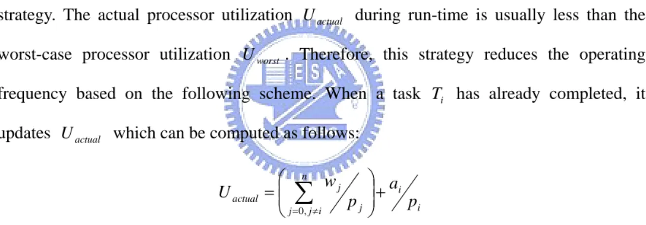
(4). Utilization updating

ccEDF [1], laEDF [1], and the algorithm proposed by Krishna et al. [9] used this strategy. The actual processor utilization during run-time is usually less than the worst-case processor utilization . Therefore, this strategy reduces the operating frequency based on the following scheme. When a task has already completed, it updates which can be computed as follows:

actual U worst U i T actual U i i n i j j j j actual _p a p w U _⎟⎟+ ⎠ ⎞ ⎜⎜ ⎝ ⎛ =

∑

where is the number of tasks in the task set, is the worst-case execution time of a

task , is the period of a task , and is the actual workload of . The

operating frequency is set to

n wj j T pj Tj ai Ti max f U

f = _actual × , where is the maximum CPU frequency.

max

f

2.3 Comparison of Existing Inter-Task DVS Algorithms

Table 1 shows the comparison of several existing inter-task DVS algorithms and the proposed algorithm dwDVS. The metric of scheduler indicates what scheduling policies are

used. The metric of strategy indicates that one or more slack time estimation strategies, that were described in Chapter 2.2, are used to estimate the slack time. Furthermore, a strategy with a superscript “*” means an improved version. The metric of number of preemptions indicates frequency of preemptions. The more effective of the slack time estimation results in the more number of preemptions. This is because that there are more opportunities for higher priority tasks to preempt lower priority tasks when the execution time of lower priority tasks becomes longer due to lowering the supply voltage. The metric of energy

consumption indicates the CPU energy consumption using each algorithm. In Chapter 4, we

will compare the proposed dwDVS with static voltage scaling [1], laEDF [1], and DRA [2], quantitatively. Note that dwDVS is similar to laEDF in the aspect of deferred-workload and DRA is better than the rest of existing inter-task algorithms [2].

Algorithm Scheduler Strategy Number of Preemptions Energy consumption ccRM [1] RM (1)+(2)* Medium Medium lppsRM [10] RM (1)+(2) Low High

Static [1] EDF (1) Low High

lppsEDF [10] EDF (1)+(2) Low High

ccEDF [1] EDF (4) Low High

lpSEH [8] EDF (1)+(2)+(3)* Medium Medium

laEDF [1] EDF (4)* Medium Medium

DRA [2] EDF* (1)+(2)+(3) Medium Medium dwDVS

(proposed)

EDF* (3)* High Low

Chapter 3

Proposed Deferred-workload-based

DVS (dwDVS)

3.1 System Model

The target processor can change its supply voltage and operating frequency continuously within its operational ranges, and . A task set T of periodic tasks is denoted as . Each task has its own period and worst-case execution time (WCET) . The deadline of is assumed to be equal to its period . The instance of is denoted by . Each task releases its instance periodically and all tasks are assumed to be mutually independent.

] ,

[V_min V_max [f_min,f_max] n

} ,..., , , {T1 T2 T3 Tn T = Ti pi i w d_i T_i i p jth Ti Ti,j

We consider a preemptive hard real-time system where periodic real-time tasks are scheduled under the EDF* scheduling policy [2] which is similar to the earliest deadline first (EDF) scheduling policy. The differences are as follows [2]:

z Among the tasks whose deadlines are the same, the task with the earliest arrival time has the highest priority.

z Among the tasks whose deadlines and arrival times are the same, the task with the lowest index has the highest priority, which means that if tasks and have the

same deadlines and arrival times, has a higher priority.

2 , 1 T T2,1 1 , 2 T 8

3.2 Problems of Most Existing Inter-Task DVS

Algorithms

Most of existing inter-task DVS algorithms have the following two potential problems so that their performances on reducing energy consumption are not efficient enough:

z Their slack estimation methods are too conservative, which means that they don’t take full advantage of slack time from lower priority tasks which have completed before their WCET in order to guarantee all deadlines.

z They set a high operating frequency to execute a task initially and reduce operating frequency when this task has completed before its WCET.

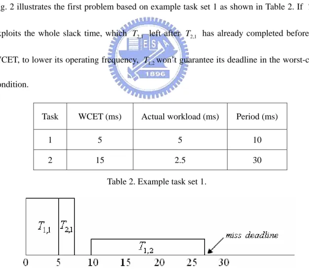
Fig. 2 illustrates the first problem based on example task set 1 as shown in Table 2. If

exploits the whole slack time, which left after has already completed before its

WCET, to lower its operating frequency, won’t guarantee its deadline in the worst-case condition. 2 , 1 T 1 , 2 T T2,1 2 , 1 T

Task WCET (ms) Actual workload (ms) Period (ms)

1 5 5 10

2 15 2.5 30

Table 2. Example task set 1.

Fig. 2. An illustration of incorrect slack time estimation from T2,1 based on example task set 1.

3.3 The Basic Idea of dwDVS

To solve the two potential problems that have been described in Chapter 3.2, we propose the following two strategies:

z We reserve a time interval for each task instance to execute its workload within this time interval even in the worst-case condition so that we can guarantee all deadlines. By determining the reserved time intervals for all task instances, we can easily estimate the slack time from either higher priority or lower priority tasks.

z We defer these reserved time intervals, which means that these reserved time intervals will be shifted to the deadline of their corresponding tasks as close as possible. By deferring the reserved time intervals, we can reduce the operating frequency without slack time.

3.4 The Detailed Procedure of dwDVS

Based on the two strategies that were described in Chapter 3.3, we design a procedure to reserve a deferred time interval for each task instance, as shown in Fig. 3, which includes steps 1 through 5, as described below. After that, the operating frequency of the task instance which is ready to execute can be determined (steps 6 and 7).

(1) Find a task Ti which has the minimum period in a task set.

(2) Find a task instance T_i,_j of Ti which has the maximum deadline di,j.

(3) Check the time intervals from to zero and determine which time interval can be

allocated to according to the following parameters:

j i d, j i T,

z The remaining worst-case execution time (RWCET) of , : When

is set to zero, the reserved time interval for is determined.

j i T, RWCET(Ti,j) ) (Ti,j RWCET Ti,j

z The state of a time interval T[k−1,k]:

¾ : It means that the time interval is not reserved for any task instances.

reserve No _

¾ : It means that only part of the time interval is reserved for one or more task instances.

reserve Partial _

¾ : It means that the whole time interval is reserved for one or more task instances.

reserve Full _

z The remaining time of a time interval T[k−1,k] , which is denoted by : If the state of a time interval

rem k k

T[ −1, ]. T[k−1,k] is , is the amount of time which is not reserved for other task instances.

reserve Partial _ rem k k T[ −1, ].

(4) Repeat steps 1 through 3 until all task instances in a task set have their corresponding reserved time intervals.

(5) The reserved time intervals should be updated by repeating steps 1 through 4 when a task has already completed or has been preempted.

(6) The time interval, which is not reserved for any task instances, is denoted by a vacant time interval (VTI), such as T[0,3] in Fig. 4(a). A task instance can take a VTI,

which appears before the deadline of , as its available execution time (AET). Then,

we can calculate the AET of , as follows:

j i T, j i T, j i T, (1) ) ( ) ( ) (Ti,j RWCET Ti,j VTI Ti,j AET = +

(7) Finally, we can set the operating frequency fdvs for Ti,j, as follows:

(2) ) ( ) ( ) ( _max , , , f T AET T RWCET T f j i j i j i dvs = ×

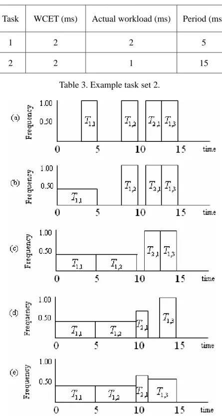
We use an example task set (Table 3) to illustrate steps 1 through 7 of dwDVS, as shown in Fig. 4. In Fig. 4(a), the deadline and RWCET of the task instance T1,3 is 15 ms

and 2 ms. The state of time interval is . We reserve the time interval for to execute its workload. In the worst-case condition, will be ready to execute at 13 ms and complete at 15 ms.

] 15 , 13 [ T No _reserve ] 15 , 13 [ T T_1,3 T1,3

Fig. 4(b) illustrates how CPU sets a proper operating frequency for a task T1,1 based on the reserved time intervals and VTI in Fig. 4(a). When has already completed at 5 ms, the reserved time intervals are updated by repeating steps 1 through 3, as shown in

1 , 1

T

Fig. 3. Fig. 4(c), and Fig. 4(d) , Fig. 4(e) can be deduced accordingly.

Find a task Ti which has the minimum period in a task set;

Find a task instance T_i,j of T which has the maximum deadline _i d_i,j;

for k =d_i,j to 0 if RWCET(T_i,j)==0 break else if T[k−1,k]==No_reserve if RWCET(T_i,j)≥1 reserve Full k k T[ −1, ]= _ 1 ) ( ) (T_i,j =RWCET T_i,j − RWCET else reserve Partial k k T[ −1, ]= _ ) ( 1 ]. , 1 [k k rem RWCET T_{i, j} T − = − 0 ) (T_i,j = RECET

else if T[k−1,k]==Partial_reserve

if (RWCET(T_i,j)+T[k−1,k].rem)>1 reserve Full k k T[ −1, ]= _ ) ]. , 1 [ 1 ( ) ( ) (T_, RWCET T_, T k k rem RWCET _{i j} = _{i j} − − −

else if (RWCET(T_i,j)+T[k−1,k].rem)==1 then

reserve Full k k T[ −1, ]= _ 0 ) (T_i,j = RWCET else reserve Partial k k T[ −1, ]= _ RWCET(T_i,j)=0

Task WCET (ms) Actual workload (ms) Period (ms)

1 2 2 5

2 2 1 15

Table 3. Example task set 2.

Fig. 4. An illustration of dwDVS based on example task set 2: (a) Initialize to reserve deferred time intervals; (b) Set the operating frequency for T1,1 based on equations 1 and 2 that were described in Chapter 3.4; (c), (d), (e): Update the reserved time intervals after T1,1, T1,2, and T2,1 have already completed, respectively. Then, set a proper operating frequency for T1,2, T2,1, and T1,3, respectively.

Chapter 4

Simulation Results and Discussion

4.1 Classical Inter-Task DVS Algorithms

To evaluate the proposed dwDVS, we have implemented the following inter-task DVS algorithms:

z Static voltage scaling (Static) [1]:

This algorithm is proposed by Pillai and Shin. The CPU runs at a lowest possible constant CPU frequency to guarantee all deadlines.

z Look-ahead EDF (laEDF) [1]:

This algorithm is also proposed by Pillai and Shin. It uses a modified utilization updating strategy, such that it estimates the minimum workloads required to be executed before the latest deadline.

z Dynamic reclaiming algorithm (DRA) [2]:

This algorithm is proposed by Aydin and Melhem. It integrates the maximum constant speed, stretching to NTA, and priority-based slack stealing strategies.

z Theoretical low bound (Bound):

This is an oracle algorithm, which knows the actual workload of each task in advance and uses an optimal speed schedule.

4.2 Simulation Model

In the simulations, we assumed the processor can change its operating frequency and supply voltage continuously within its operational ranges, [fmin,fmax] and [Vmin,Vmax] [2].

The actual workload of each task instance is drawn from a normal distribution with mean

2

WCET BCET +

and standard deviation

6

BCET WCET −

[2], where BCET is the

best-case execution time, meaning that 99.7% of the actual workload falls in the interval . If the actual workload is less than BCET or greater than WCET, we set it

to BCET or WCET, respectively. In the following, we compare the average energy

consumption of these algorithms, which is normalized to the average energy consumption of

Static

] ,

[BCET WCET

[1], under different conditions.

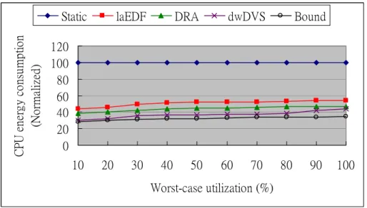
4.3 Effect of Worst-Case Utilization on Energy

Consumption

Fig. 5 compares the average energy consumption of each inter-task DVS algorithm under different worst-case utilization. The number of task sets is 100, the number of tasks in a task set is 8, the

BCET WCET

ratio is 5, and the worst-case utilization varies from 10% to 100% [2]. From these simulation results, we have the following two observations:

z The dwDVS reduces the energy consumption by an average of 63%, 14%, and 7% compared with the Static [1], laEDF [1] and DRA [2] algorithms, respectively.

z When the worst-case utilization is greater than 90%, the improvement of dwDVS on reducing the energy consumption is not as obvious as the cases with the worst-case utilization of less than 90%. This is because that the advantage , which is generated from

reserving deferred time intervals by dwDVS, is limited under high worst-case utilization. 0 20 40 60 80 100 120 10 20 30 40 50 60 70 80 90 100 Worst-case utilization (%) C P U en er g y co ns u m p tio n (N or m al iz ed)

Static laEDF DRA dwDVS Bound

Fig. 5. Effect of worst-case utilization on energy consumption.

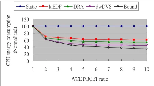
4.4 Effect of WCET/BCET Ratio on Energy

Consumption

Fig. 6 compares the average energy consumption of each inter-task DVS algorithm under various

BCET WCET

ratio. The number of task sets is 100, the number of tasks in a task set is 8,

the worst-case utilization is 60%, and the

BCET WCET

ratio varies from 1 to 10 [2]. From these simulation results, we have the following two observations:

z The dwDVS reduces the energy consumption by an average of 52%, 13% and 9% compared with laEDF [1] and DRA [2], respectively.

z When >5

BCET WCET

, the improvement on energy consumption is not obvious as that of

5 ≤

BCET WCET

. This is because that the expected workload converges rapidly to 50% of the

worst-case workload with the increasing

BCET WCET

0 20 40 60 80 100 120 1 2 3 4 5 6 7 8 9 10 WCET/BCET ratio C P U en er g y co ns u m p tio n (N or m al iz ed)

Static laEDF DRA dwDVS Bound

Fig. 6. Effect of WCET/BCET ratio (actual workload) on energy consumption.

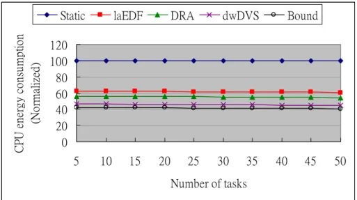
4.5 Effect of Number of Tasks in a Task Sets on Energy

Consumption

Fig. 7 compares the average energy consumption of each inter-task DVS algorithm with respect to a different number of tasks in a task set. The number of task sets is 100, the worst-case utilization is 60%, the

BCET WCET

ratio is 5, and the number of tasks in a task set varies from 5 to 50. From these simulation results, we observe that the energy consumption of each inter-task DVS algorithm decreases slightly when the number of tasks in a task set increases. This is because that the overall workloads rely on the actual workload of each task instance and the worst-case utilization, but not on the number of tasks in a task set. However, the energy consumption indeed decreases when the number of tasks in a task set increases. This is because when the number of tasks in a task increases, each inter-task DVS algorithm has more task instances from which slack time is available.

0 20 40 60 80 100 120 5 10 15 20 25 30 35 40 45 50 Number of tasks C P U en er g y co ns u m p tio n (N or m al iz ed)

Static laEDF DRA dwDVS Bound

Chapter 5

Conclusions and Future Work

5.1 Concluding Remarks

In this thesis, we have presented an energy-efficient inter-task DVS algorithm called

dwDVS based on deferred-workload. The proposed dwDVS is motivated by the observation

that most of existing inter-task DVS algorithms run at a higher frequency initially and estimate the slack time from lower priority tasks too conservative. The main contribution of the proposed dwDVS is that the slack time from lower priority tasks can be efficiently estimated and the CPU frequency can be reduced even without slack time. The overheads of our approaches are an increase in number of preemptions, which results in increasing the energy consumption in memory subsystems, and extra energy consumption and time for voltage transitions. Fortunately, these overheads are usually small enough and thus can be neglected [1][7][8][9]. Simulation results have shown that dwDVS can effectively reduce the energy consumption by 40-70%, 10-20%, and 3-10% compared with Static [1], laEDF [1] and DRA [2] algorithms, respectively, and approaches the theoretical low bound by a margin of at most 12%.

5.2 Future Work

A more intelligent slack time distribution for more tasks instead of one can be used to further improve the proposed dwDVS. It means that if a higher priority task has completed before its deadline, the slack time which left need not be allocated fully to the next lower priority . We may distribute the slack time to the next two or more lower priority tasks based on a clever strategy, such as a profile-based slack time distribution

i T i T j T 20

strategy. In addition, we may take more factors, such as number of preemptions or extra time and energy consumption for voltage transitions, into consideration to make the system model of the proposed dwDVS more close to realistic systems. The effectiveness of these strategies deserve to further study.

Bibliography

[1] P. Pillai and K.G. Shin. “Real-Time Dynamic Voltage Scaling for Low-Power Embedded Operating Systems,” in Proceedings of 18th ACM Symposium on Operating

Systems. pp. 89-102, October 2001.

[2] H. Aydin, R. Melhem, D. Moose, and P. Mejia-Alvarez, “Power-Aware Scheduling for Periodic Real-Time Tasks,” IEEE Transactions on Computers, Volume 53, Issue 5, pp. 584-600, May 2004.

[3] B. Moyer, “Low-Power Design for Embedded Processors,” in Proceedings of IEEE, Volume 89, Issue 11, pp. 1576-1587, November 2001.

[4] Intel, PXA255 Processor Electrical, Mechanical, and Thermal Specification, 2004. [5] Intel, PXA270 Processor Electrical, Mechanical, and Thermal Specification, 2004. [6] Transmeta Corporation, http://www.transmeta.com/

[7] W. Kim, D. Shin, H. S. Yun, S. L. Min, and J. Kim. ”Performance Comparison of Dynamic Voltage Scaling Algorithms for Hard Real-Time Systems,” in Proceedings of

the IEEE Real-Time and Embedded Technology and Application Symposium, pp.

219-228, September 2002.

[8] W. Kim, J Kim, and S. L. Min. “A Dynamic Voltage Scaling Algorithm for Dynamic Priority Hard Real-Time Systems Using Slack Time Analysis,” in Proceedings of

Design, Automation and Test in Europe, pp. 788-794, March 2002.

[9] C. M. Krishna and Y. H. Lee, “Voltage Clock Scaling Adaptive Scheduling Techniques for Low Power in Hard Real-Time Systems,” IEEE Transactions on

Computers, Volume 50, Issue 8, pp. 1586-1593, August 2003.

[10] Y. Shin, K. Choi, and T. Sakurai. “Power Optimization of Real-Time Embedded Systems on Variable Speed Processors,” in Proceedings of the International

Conference on Computer-Aided Design, pp. 365-368, June 2000.

[11] R. Venkat, G. Singhal, and A. Kumar, “Real-Time Dynamic Voltage Scaling for Embedded Systems,” in Proceeding of the 17th International Conference on VLSI

Design, pp. 650-653, 2004.

[12] F. Gruian, “Hard Real-Time Scheduling for Low-Energy Using Stochastic Data and DVS Processors,” in Proceeding of ISLPED, pp. 849-864, August 2001.

[13] D. Shin, S. Lee, and J. Kim, “Intra–Task Voltage Scheduling for Low-Energy Hard Real-Time Applications,” IEEE Design and Test of Computers, pp. 20-30, March 2001.

[14] J. R. Lorch and A. J. Smith, “PACE: A New Approach to Dynamic Voltage Scaling ,”

IEEE Transactions on Computers, Volume 53, Issue 7, pp. 856-869, July 2004.

[15] J. Lehoczkym L. Sha, and Y. Ding, “The Rate Monotonic Scheduling Algorithm: Exact Characterization and Average Case Behavior,” in Proceedings of the IEEE

Real-Time Systems Symposium, pp. 166-171, December 1989.

[16] C. L. Liu and J. W. Leyland, “Scheduling Algorithms for Multiprogramming in A Hard Real-Time Environment,” Journal of the ACM, pp. 46-61, January 1973.