國 立 交 通 大 學
電信工程學系
碩 士 論 文
在以封包為基底的傳輸系統下
對影像串流之平順演算法
Smoothing Algorithm for Video Streaming
in Packet Based Transmission System
研究生 : 林旃偉
指導教授 : 張文鐘 博士
在以封包為單位的傳輸系統下
對影像串流之平順演算法
Smoothing Algorithm for Video Streaming
in Packet Based Transmission System
研 究 生:林旃偉
Student:Chan-Wei Lin指導教授:張文鐘
Advisor:Wen-Thong Chang國 立 交 通 大 學
電 信 工 程 系
碩 士 論 文
A ThesisSubmitted to Department of Communication Engineering College of Electrical Engineering and Computer Science
National Chiao Tung University in partial Fulfillment of the Requirements
for the Degree of Master
in
Communication Engineering
August 2005
Hsinchu, Taiwan, Republic of China
在以封包為單位的傳輸系統下
對影像串流之平順演算法
研究生: 林旃偉 指導教授: 張文鐘 博士
國立交通大學電信工程學系碩士班
中文摘要
電腦網路技術的提升,使得整合性應用的服務增加。影像串流被認為
未來網路影用的主要部份。網路必須分送不同的影像資料以滿足不同的應
用,例如,包含聲音的即時影像要求、多媒體短片與電影。這類本身含有
大量突衝以及速率變動的資料流,加重網路的負載,同時降低了網路的使
用效率,也使得網路的管理更加困難。因此,為克服這些問題,發展了能
降低資料流突衝的平順演算法。然而,傳統的平順演算法,並無法與影像
壓縮標準完美地結合。在此我們提出了兩種以封包為基底的平順演算法。
這兩個以封包為基底的平順演算法,能夠近似傳統平順演算法,同時能在
不對影像壓縮標準作修正的情形下被實現。在這篇論文中,我們介紹了我
們的以封包為基底的平順演算法,展示他的模擬結果以及演算法的效能。
Smoothing Algorithm for Video Streaming
in Packet Based Transmission System
Student: Chan-Wei Lin Advisor: Dr. Wen-Thong Chang
The Department of Communication Engineering National Chiao Tung University
Abstract
The improvement of the computer network technologies result in the increasing of application of integrated services. The video stream is expected to be the major portion of the network application. Network has to deliver various numbers of video data traffic for several applications such as Video on Demand, which contains audio, multimedia clip and movies. This kind of traffic, which has much burst and variable rate inherently, increases the load of network service, decreases the efficiency of network utilization and also makes the network management difficult. Therefore, to overcome these difficulties, the smoothing algorithms, which reduce the burst of traffic, are developed. However, the conventional smoothing algorithm cannot combine with the video compression standards perfectly. We proposed two packet-based smoothing algorithms. These two algorithms approximate to the conventional smoothing algorithm, and can be implemented without modifying the video compression algorithm. We introduce our packet-based smoothing algorithms, show the simulation result and also demonstrate the performance in this thesis.
Acknowledgement
三年的碩士班生涯,即將在這裡告一個段落。從一開始對未來的迷惘,
到認清事實,然後逐步走上軌道,這段過程都將成為我人生中很重要的一
個階段吧。
必須感謝我的父母,在這段時間完全放手的讓我去尋找自己的道路,
也因為有你們的支持,我才能無後顧之憂。感謝指導教授張文鐘教授,口
試委員范國清教授、余孝先主任和李安謙教授,你們的指導,讓我的論文
更趨完整。實驗室的夥伴們、學長姐們,從你們那裡學到了許多,也得到
了很多的照顧,不成熟的我,如果能在未來有些許的成長,是多虧了與你
們的相處。
高中時期的好朋友們,在我對將來感到迷惘的這個時期、在碩士生涯
的無數個低潮,有你們的陪伴和鼓勵,那些接近無厘頭的相處和對談,讓
我能完全的放鬆,用更開闊的心胸面對生活上的挑戰。傅思維、猪、狗、
五百、井長瑞,很感謝你們。最後這一兩個月,大概是這三年來最難熬的
時候,修改論文上遇到的種種困難,讓自己很想在最後關頭放棄,之所以
能重新站起來走到最後,猛男、系花、蕃薯,多虧了有你們的鼓勵。
這段過程,看到了許許多多的人生百態,有無數需要感謝的人,不論
是好是壞,所有帶給我人生歷練的一切,都感謝你們。感謝上天,讓我在
學生生涯的最後,遇見了蕙君,讓一切的努力都逐漸出現了目標,也讓未
Content
中文摘要 ... i Abstract ... ii Acknowledgement ... iii Content...v List of Figures... vi 1. Introduction...12. Conventional Smooth Algorithm ...3
2.1 Buffer Constrained Smoothing Algorithm ...4
2.1.1 Overflow and Underflow Constrain...4
2.1.2 Minimum Variability Bandwidth Allocation (MVBA) ...7
2.2 Rate Constrained Smoothing Algorithm ...13
2.2.1 Rate Constrained Bandwidth Smoothing (RCBS) ...15
3. Simulation and Performance Evaluation of MVBA ...18
3.1 Simulation Setting ...18
3.2 Performance of MVBA...19
4. Packet based Smoothing Algorithm...28
4.1 Number-of-Packets Based Smoothing Algorithm ...30
4.1.1 Modification of Upper Bound in Packet Based Smoothing Algorithm .30 4.1.2 Modification of integer transmission rate ...35
4.1.3 The procedure of Number-of-Packets based smoothing algorithm ....37
4.2 Packet Mapped Smoothing Algorithm ...38
4.2.1 Upper and Lower Bound in Optimum Transmission Schedule ...38
4.2.2 The procedure of Packet Mapped smoothing algorithm ...40
4.3 Implementation of Packet Based Smoothing Algorithm...40
5. Simulation of Packet Based Smoothing Algorithm...43
5.1 Performance of Number-of-Packets Based Smoothing Algorithm ...43
5.2 Performance of Packet Mapped Smoothing Algorithm ...58
5.3 Influence of Maximum Packet Sizes...74
5.4 Implementation Result...80
6. Conclusion...93
List of Figures
Figure 1 An example of transmission schedule...3
Figure 2 An example of feasible and infeasible transmission schedules...6
Figure 3 An example of , mina b s , , maxa b s , and corresponding , a b L t , , a b U t ...10
Figure 4 An example of a condition in which the feasible CBR transmission schedules exist...10
Figure 5 The condition of buffer overflowing and underflowing...12
Figure 6 An example of feasible rate constrained transmission schedule……....14
Figure 7 An example of RCBS procedure...17
Figure 8 The transmission schedule of MVBA with different client buffer...20
Figure 9 Peak rate of transmission schedule generated by MVBA with 100K bits client buffer size...22
Figure 10 Transmission schedule of other video trace...25
Figure 11 The statistical data of smoothed transmission schedule...26
Figure 12 An example of transmission schedule in packet format...29
Figure 13 The difference of upper bound and lower bound between conventional smoothing algorithm and packet based smoothing algorithm...32
Figure 14 The upper bound and lower bound of packet number in packet based smoothing algorithm...33
Figure 15 The modification of integer transmission rate...36
Figure 16 An example of number of packets controlled rate control...39
Figure 17 Block diagram of a video transmission server with packet based smoothing algorithm...42
Figure 18 The modified upper bound and lower bound of “Aladdin” with 32K client buffer and 1024 bits maximum packet size...44
Figure 19 The modified upper bound and lower bound of “Aladdin” with 32K client buffer and 2048 bits maximum packet size...45
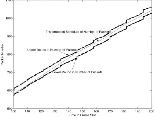
Figure 20 Transmission schedule of number of packets of “Aladdin” with 32K bits client buffer and 1024 bits maximum packet size...46
Figure 21 Transmission schedule of number of packets of “Aladdin” with 32K bits client buffer and 2048 bits maximum packet size...47
Figure 24 Transmission rates of the first 1000 frames of “Aladdin” generated by Number-of-Packets Based Smoothing Algorithm with 32k bits client buffer and 1024 bits maximum packet size...49 Figure 25 Transmission rates of the first 1000 frames of “Aladdin” generated by
Number-of-Packets Based Smoothing Algorithm with 32k bits client buffer and 2048 bits maximum packet size...50 Figure 26 The transmission rate of the total video “Aladdin” generated by
Number-of-Packets Based Smoothing Algorithm with 100k bits client buffer and 1024 bits maximum packet size...51 Figure 27 The transmission rate of the total video “Aladdin” generated by
Number-of-Packets Based Smoothing Algorithm with 1M bits client buffer and 1024 bits maximum packet size...…52 Figure 28 The transmission rate of the total video “Aladdin” generated by
Number-of-Packets Based Smoothing Algorithm with 100k bits client buffer and 2048 bits maximum packet size...53 Figure 29 The transmission rate of the total video “Aladdin” generated by
Number-of-Packets Based Smoothing Algorithm with 1M bits client buffer and 2048 bits maximum packet size...…..54 Figure 30 The variance in transmission rate smoothed by Number-of-Packets
Based Smoothing Algorithm as a function of client buffer...…56
Figure 31 The peak rate smoothed by Number-of-Packets Based Smoothing
Algorithm as the function of client buffer...57
Figure 32 The BFF of the schedule smoothed by Number-of-Packets Based
Smoothing Algorithm as the function of client buffer...58
Figure 33 Transmission schedule generated by MVBA and by Packet Mapped
Smoothing algorithm with 32K bits client buffer and 1024 bits maximum packet size under
,
mina b
s condition...59
Figure 34 Transmission schedule generated by MVBA and by Packet Mapped
Smoothing algorithm with 32K bits client buffer and 2048 bits maximum packet size under
,
mina b
s condition...60
Figure 35 Transmission schedule generated by MVBA and by Packet Mapped
Smoothing algorithm with 32K bits client buffer and 1024 bits maximum packet size under
,
maxa b
s condition...61
Figure 36 Transmission schedule generated by MVBA and by Packet Mapped
packet size under
,
maxa b
s condition...62 Figure 37 The transmission rate of first 1000 frames of “Aladdin” generated by
Packet Mapped smoothing algorithm with 32K bits client buffer and 1024 bits maximum packet size...64 Figure 38 The transmission rate of first 1000 frames of “Aladdin” generated by
Packet Mapped smoothing algorithm with 32K bits client buffer and 2048 bits maximum packet size...65 Figure 39 The transmission rate of total video of “Aladdin” generated by Packet
Mapped smoothing algorithm with 100K bits client buffer and 1024 bits maximum packet size...66 Figure 40 The transmission rate of total video of “Aladdin” generated by Packet
Mapped smoothing algorithm with 100K bits client buffer and 2048 bits maximum packet size...67 Figure 41 The transmission rate of the total video “Aladdin” generated by Packet Mapped smoothing algorithm with 1M bits client buffer and 1024 bits maximum packet size...68 Figure 42 The transmission rate of first total video “Aladdin” generated by Packet Mapped smoothing algorithm with 1M bits client buffer and 2048 bits maximum packet size...69
Figure 43 The variance in transmission rate smoothed by packet mapped
smoothing algorithm as a function of client buffer...71 Figure 44 The graph illustrates the peak rate smoothed by packet mapped
smoothing algorithm as the function of client buffer...72 Figure 45 The graph illustrates the BFF of the schedule smoothed by packet
mapped smoothing algorithm as the function of client buffer...72 Figure 46 The total number of packets as a function of maximum packet size…..75 Figure 47 The total number of packets as a function of maximum packet size to mean rate ratio...76 Figure 48 The variance of all packet size...77 Figure 49 The variance of small packet size, which is not full...78 Figure 50 The variance of rate difference between MVBA schedule and Packet
Mapped Smoothing Algorithm...79 Figure 51 The record of the packet size and time...81
detail...85 Figure 57 The record of the packet size and time with unsmoothed schedule from
NCTU to CCU...86 Figure 58 The record of the packet size and time with unsmoothed schedule from
NCTU to CCU in detail...86 Figure 59 Histogram of group interval with smoothed schedule form NCTU to
NCTU...87 Figure 60 Histogram of group interval with smoothed schedule form NCTU to
CCU...87 Figure 61 Histogram of group interval with unsmoothed schedule form NCTU to
NCTU...88 Figure 62 Histogram of group interval with unsmoothed schedule form NCTU to
CCU...89 Figure 63 Histogram of packet interval with smoothed schedule form NCTU to
NCTU...90 Figure 64 Histogram of packet interval with smoothed schedule form NCTU to
CCU...90 Figure 65 Histogram of packet interval with unsmoothed schedule form NCTU to
NCTU...91 Figure 66 Histogram of packet interval with unsmoothed schedule form NCTU to
1. Introduction
Due to the increasing of network bandwidth, multimedia applications, such as video casting, video-based entertainment, and video on demand, become more and more. These applications consume a substantial amount of network bandwidth. Although Video which compressed in constant bit rate (CBR) is easier to network service, the picture quality will vary with the content of video. If the complexity of the picture content or the motion of video is higher, the picture quality will reduce significantly. On the contrary, if the picture quality is maintained, the rate will vary with the content. Also, the compression technique which introduces the method, that compress I, P, B, three different frame types in different way, result in data burst and rate variation. This kind of variable bit rate (VBR) data waste the network resources and lower the bandwidth utilization efficiency, as it is transmitted through network directly. For overcoming this difficulty, smoothing algorithms are developed. In order to access network bandwidth efficiently and manage easily, the transmission of streams data tends to be transmitted in CBR. Thus the VBR data streams have to be modified into low burst and rate variation. To transmit VBR stream through network in CBR is the main function of smoothing algorithm.
In order to access network bandwidth efficiently and manage easily, the transmission of streams data tends to be transmitted in CBR. To transmit VBR stream through network in CBR is the main function of smoothing algorithm. Many smoothing algorithms are proposed to reduce the variation in transmission rate. But these
to smoothing algorithm can't match the optimum transmission schedule generated by smoothing algorithm perfectly. If the video has to be transmitted according to the transmission schedule, the packets have to be segmented again by server, and be reassembled by client. The segmenting and reassembling mechanisms are not defined in video compression standards. It will limit the application of smoothing algorithm. We proposed two packet-based smoothing algorithms to approximate performance of the conventional smoothing algorithm with the method to control the transmitted number of packets at each frame slot.
In the following section, one buffer constrained smoothing algorithm, minimum variance bandwidth allocation (MVBA)[2][3][4][5], and one rate constrained smoothing algorithm, rate constrained bandwidth smoothing (RCBS) [7][14], is introduced and its performance is shown in section 2 and 3. Our packet based smoothing is related in section 4, and section 5 includes the simulation result and performance of our algorithm. Finally, a conclusion is presented in the last section.
2. Conventional Smooth Algorithm
Now, we describe the framework of video streaming. First step of the procedure of video stream transmission is that client sends a demand to the server, and the connection is established. Server accesses the video data from the storage device, and then sends the video data through the network to the client. The client will store up this data in the buffer, and extract them to send to the decoder according to the playback schedule. The traditional method is that server sends each frame data at each corresponding frame slot. A streaming server with smoothing algorithm can transmit video data at a more stable rate. Instead of transmitting each frame data at each corresponding frame slot, the server will reschedule the transmission data at each frame slot. The large frame, such as I frame, may be cut into several portions and transmitted ahead at the previous frame slot, and the small frame, such as P or B frame, may be transmitted together at one frame slot. For instance, an I frame may be cut into several part and be transmitted at the previous P or B frame slots. See the following Fig. 1 as an example. The large I frame data is cut into two segments, and one of them is transmitted at the B frame slot, and two B frames are transmitted at a frame slot.
Because of the real time property of video streaming, transmission schedule is under the following restrictions. If the transmission rate is too low, the client buffer will be underflowing, and it will induce the playback delay. On the contrary, if the transmission rate is too high, the client buffer will overflow, and it will induce the loss of data and frame drop. Therefore, although the ultimate goal of smoothing algorithm is to find a CBR transmission schedule, but CBR schedule is usually infeasible because it may disobey the upper bound and lower bound. The rate of a feasible transmission schedule can’t be too low or too great in order to play fluently at client. Thus a feasible transmission schedule has to obey some constraints, these will describe in the following sections.
2.1 Buffer Constrained Smoothing Algorithm
First, we discuss the buffer constrained smoothing algorithm. This kind of algorithm is to find a feasible schedule with a given fixed client buffer.
2.1.1 Overflow and Underflow Constrain
At first, we describe the restriction of the transmission schedule in buffer constrained smoothing algorithm. Because the client buffer is fixed, the transmitted data can’t be too many to store up. However, the client has to receive enough data to play fluently, thus the transmitted data can’t be too less. Therefore, the total transmitted data have to obey some upper bound and lower bound. The following is the mathematic representation of the upper bound and lower bound.
At first, we describe the notation of the parameter of a video. A compressed video stream consists of N frames, and the amount of data of frame i is a bits (or bytes) to i store. Without loss of generality, we assume that time is measured in unit of frame slots. In order to playback streaming video fluently at client terminal, the server always has to send enough data to the client to prevent buffer underflowing. Thus, the lower bound of transmission schedule,
0 ( ) k i i L k a = =
∑
, for all 0<k<N (2-1)The sum of ai for the duration of 0 to k represents the amount of data consumed at the client during k frame slots. The server has to transmitted at least L(k) to client in order to confirm that the client always has enough data to play.
Also, a client cannot receive too many data to store. The remainder data, which subtract the consumed data from the total transmitted data, can’t be greater than the client buffer size to prevent buffer overflowing. Thus the upper bound of transmission schedule,
( ) ( )
U k =L k + , b (2-2)
where b is the client buffer size. The sum of L(k) and b represents that the total amount of data which is transmitted by server cannot exceed the total consumed data at client plus buffer size to prevent buffer overflow. The total transmitted data can’t be above U(k), or the remainder data after the client consume the video data will be
enclosed by the upper bound and lower bound. That is, 0 ( ) ( ) k i i L k s U k = ≤
∑
≤ , for all 0<k<N (2-3)where si is the transmission rate of the schedule of the smoothed video stream at frame slot i.
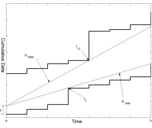
Figure.2: An example of feasible and infeasible transmission schedules.
feasible transmission schedule has to stay inside upper bound and lower bound, otherwise, the schedule is infeasible, and the slope of each segment indicates the transmission rate during each corresponding period. Fig.2 is an illustration of feasible and infeasible transmission schedule. Where the two bold solid lines represent the upper and lower bound, the fine solid line is a feasible transmission schedule, and dot line is an infeasible transmission schedule which result in client buffer overflowing at the prior segment and buffer underflowing at the later segment.
2.1.2 Minimum Variability Bandwidth Allocation (MVBA)
In this paper, we introduce one of the buffer constrained smoothing algorithms, MVBA. The criterion of this algorithm is to minimize the variance in transmission rate. The transmission schedule resulted by MVBA has the following properties.
1. The rate variation is minimized.
2. The peak rate is minimized.
3. The lowest rate is maximized.
MVBA will find a succession of feasible CBR segments. These segments connect with each other at the end points. Then the transmission schedule generated by MVBA consists of these CBR segments, and the slopes of each segments represents
change the rate slightly to find the successive feasible CBR segment as early as possible. The new segment will start at the time that the client buffer is just overflowing or just underflowing when the process find that the CBR segment will be infeasible in the future, and the process will repeat until whole video is be segmented. The variance of rate of the transmission schedule generated by MVBA will be minimized. The proof of this property is described in [2].
The Parameters of MVBA
At first, we define the parameters of the MVBA. Let
,
maxa b
s segment represents
the maximum transmission rate without making client buffer full in the interval [a,b]. The CBR segment starts with initial buffer level q, which is the remainder data stored in client buffer at ath frame slot when the process starts a new run from ath frame slot.
That is , max 1 ( ) ( ( ) ) min a b a t b U t L a q s t a + ≤ ≤ − + = − , (2-4)
and tUa b, is the latest frame slot at which client buffer is full when server transmit at
the rate of smaxa b, in interval [a,b]. That is
, 1 max ( ) ( ( ) ) max : a b U a t b U t L a q t t s t a + ≤ ≤ − + ⎧ ⎫ = ⎨ = ⎬ − ⎩ ⎭. (2-5)
For each interval [a,b], there exist only one smaxa b, segment and one
lower bound of transmission schedule. smaxa b, segment starts at ath frame slot with
initial buffer level q. At the interval [a,a+4], [a,a+5], [a,a+6], [a,b], the smaxa b, is
invariant, and the corresponding tUa b, is also the same.
Similarly, let smina b, segment represents the minimum transmission rate without
making client buffer starve in the interval [a,b], starting with initial buffer level q:
, min 1 ( ) ( ( ) ) max a b a t b L t L a q s t a + ≤ ≤ − + = − , (2-6) and , a b L
t is the latest frame slot at which client buffer is starve when server transmit in rate
,
mina b
s in interval [a,b]. That is
, 1 min ( ) ( ( ) ) max : a b L a t b L t L a q t t s t a + ≤ ≤ − + ⎧ ⎫ = ⎨ = ⎬ − ⎩ ⎭. (2-7)
Similarly, see the
,
mina b
s segment in Fig. 3 as an example. This segment start at ath frame slot with initial buffer level q, and the client buffer will starve at tLa b, .
There exist some feasible CBR transmission schedule in interval [a,b], if and only if smax ≥smin. See Fig. 4 as an example.
Figure 3: An example of , mina b s , , maxa b s , and corresponding , a b L t , , a b U t . Time Cumula tiv e Da ta
Figure 4: An example of a condition in which the feasible CBR transmission schedules exist.
The procedure of MVBA
The process starts in the interval [1,2], where a equals to 1 and b equals to 2, and calculates , mina b s , , maxa b s , , a b L t , , a b U t and , 1 mina b s + , , 1 maxa b
s + . Then the process will check
if the following two conditions occur.
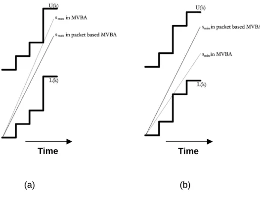
1) If the computed smaxa b,+1 at [a,b+1] is smaller than smina b, , it's means that
if server transmits data in rate smina b, at [a,b+1], the client buffer will
overflow at b+1th frame slot. See Fig. 5(a) as an example. The slope of
, mina b s is greater than + , 1 maxa b s , thus , mina b
s will reach the upper bound at b+1th frame slot. This phenomenon represents that the client buffer is
overflowing at b+1th frame slot. Thus the transmission rate must slow
down before b+1th frame slot, if the server transmits in rate
,
mina b
s from
ath frame slot. MVBA algorithm determines to transmit in rate
, mina b s at [a, , a b L
t ] , and the process starts a new computation procedure from
, a b L t , then a is set to be , a b L t and b is set to be , 1 a b L
t + . Then the initial buffer level q is set to 0.
, maxa b s is smaller than , 1 mina b s + , thus , maxa b
s will reach the lower bound at b+1th frame slot. This phenomenon represents that the client buffer is
underflowing at b+1th frame slot. Thus the transmission rate must speed
up before b+1th frame slot, if the server transmits in rate
,
maxa b
s from ath
frame slot. MVBA algorithm determines to transmit in rate smaxa b, at
[a,tUa b, ], and the process starts a new computation procedure from tUa b, ,
then a is set to be tUa b, and b is set to be tLa b, +1. Then the initial buffer
level q is set to b, the client buffer size.
Time Cumula tiv e Da ta Time Cumula tiv e Da ta (a) (b)
Figure 5: (a) represents that when smina b, ≥smaxa b,+1, client buffer will overflow at b+1th
frame slot. (b) represents that when smaxa b, ≤smina b,+1, client buffer will underflow at
Otherwise there exists a feasible CBR segment over [a, b+1], then the extension of the interval continues, b is updated to b+1, and smax, smin andt , U tLkeep on being updated. The process continues until the entire video is segmented. As b reaches to the end of the video, then b equals to N, and the last segment is just the mean rate in interval [a, N], which equals to L N( ) L a( ) q
N a
− +
− . The generated transmission schedule is identified as a series of CBR transmission segments, each ending with a change in transmission rate.
2.2 Rate Constrained Smoothing Algorithm
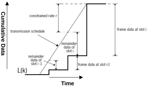
Now, we consider the rate constrained smoothing algorithm. In this case, the max transmission rate of the network link between server and client is constrained to be under r. Thus, the client buffer have to be large enough to store the data which is transmitted ahead to prevent the playback discontinuously, and the playback startup delay has to be long enough to confirm that the server can transmitted enough data ahead for the first peak of the video data with a rate that is lower than r. See Fig. 6 as an example of a feasible rate constrained transmission schedule. The minimum buffer requirement is the greatest distance between the transmission schedule and the consumed data, L(k). The server has to transmit enough data before the client starts to play the video to prevent the total transmitted data may be below L(k) in the future, and the rate for this duration has to be also lower than r. Thus the startup delay has to
Figure 6: An example of feasible rate constrained transmission schedule. The slopes of each segment have to be under r, and the cumulative transmission data have to be greater than the L(k). There exist on minimum buffer requirement and one minimum startup delay for each feasible transmission schedule, and the two parameters will be determined after the schedule is generated.
Under this constraint, a feasible transmission schedule must satisfy the following two terms: = ≥
∑
1 ( ) k i i s L k , and (2-8) ≤ i s r , for all i . (2-9)2.2.1 Rate Constrained Bandwidth Smoothing (RCBS)
RCBS, a rate constrained smoothing algorithm, is to find a transmission schedule, which transmits data as late as possible to reduce the requirement of client buffer, and also obey the rate constraint r simultaneously. After a feasible transmission schedule is computed, a corresponding group of minimum startup delay and minimum client buffer requirement is determined.
The procedure of RCBS is simple. The concept of this algorithm is that when the amount of data which must be transmitted at ith frame slot is greater than r, the server
can only transmits in rate of r at ith frame slot, and the remainder data that can’t be
transmitted at this frame slot have to be transmitted at the earlier frame slot for preventing client buffer underflowing. Therefore, the amount of data, which has to be transmitted at i-1th frame slot, becomes the data of i-1th frame plus the remainder data
of ith frame slot. The transmission schedule is as following:
+ > ⎧ = ⎨ + + < ⎩ i i i i i i i r if a rem r s a rem if a rem r . (2-10)
where a is the amount of data of ii th frame, and remi represents remainder data that have to be transmitted at i+1th frame slot originally, but the server cannot transmit
these data at i+1th frame slot because of the rate constraint. Therefore ai +remi
represents the data have to be transmitted at ith frame slot. If ai +remi is greater than
equals to ai +remi −si.
The Procedure of RCBS
The initial setting of RCBS is that i equals to N, the latest frame number, and the initial remi equals to 0, it also means that rem equals to 0. Then, according to N equation 2-10, s equals to N a and N remN−1 equals to 0 if aN +remN is smaller than r. On the other hand, if aN +remN is greater than r, s will be set to r and N
1
N
rem − will be set to aN +remN −r . Then, the next step is to check if aN−1+remN−1 is greater than r, and determine sN−1 according to equation 2-10. This process will repeat until i reaches 0. Then the total transmission schedule is generated, and the minimum buffer requirement and the minimum start up delay will be determined.
Fig. 7 illustrates this procedure, where the bold line represents L(k), and the fine line is the CBR segment of transmission schedule, of which the slope equals to r. The remainder data at ith frame slot equals to 0, therefore the data have to be transmitted
at ith frame slot equals to the data of ith frame. Because the amount of data of ith frame
is greater than the constrained rate, the server can only transmit in rate of r at ith frame
slot, and the data, which can’t be transmitted at ith frame slot, have to be transmitted at
previous frame slot. These remainder data and the data of i-1th frame have to be
transmitted together at i-1th frame slot. Then the process checks if the sum of the
remainder data and the data of i-1th frame is greater than r. If the sum is smaller than r,
the server can transmitted all of these data at this frame slot. Otherwise, like Fig. 7, the server can only transmitted in rate of r at i-1th frame slot, and the remainder data
will be transmitted at i-2th frame slot with the data of i-2th frame slot, and repeat the
same check process. This process will continuous until the whole video frame is checked.
Time Cumula tiv e Da ta
Figure 7: An example of RCBS procedure. The data exceeds the constrained rate is transmitted at the prior frame slot.
After the transmission schedule is determined, the maximum difference between transmission schedule and L(k) is the minimum required client buffer requirement. That is ≤ ≤ = ⎧ ⎫ = ⎨ − ⎬ ⎩
∑
⎭ 1 1 max ( ) t i t N i b s L t . (2-11)And the elongate part in front of the first frame slot is the startup delay, that is
0 t rem w r = , (2-12)
where, w means the start up delay, and t rem is the data which have to be 0 transmitted before 0th frame slot. The minimum startup delay equals to the data, which
3
.
Simulation and Performance Evaluation of MVBA
In this chapter, we demonstrate some examples of MVBA, and analyze and compare their performance. Also, we measure some important factors for video streaming service, peak rate, rate variation, startup delay and corresponding client buffer requirement.
The peak rate and the variability of transmission rate affect the network efficiency significantly. The lower these factors are, the higher the network efficiency is. The startup delay and buffer requirement can be considered as the criteria of admission control, for instance, a client informs the server of the maximum available buffer and the maximum waiting time, then the server execute these smoothing procedures and decides whether the demand is admitted or not according to these factor.
3.1 Simulation Setting
We experiment on several video trace with MVBA smoothing algorithm. These video trace is from [1], in QCIF format, 30 frames per second, and compressed with MPEG4. The total length is an hour, 108,000 frames. First we use the video trace of Disney animation "Aladdin" for testing. This video trace is compressed with I-P-B quantization level 10-14-16. The compression ratio is 43.4793. The total amount of frame data is 94,429,534 bytes.
In general application, clients permit a certain startup delay. In our experimentation, the startup delay is 30 seconds, 900 frame slots to lower the
transmission rate of first run.
Finally, we experiment on three different video traces, “Jurassic Park One”, “Terminator One” and “Baseball Game”. They are all in QCIF format, compressed with MPEG4 with I,P,B quantization level 10-14-16.
3.2 Performance of MVBA
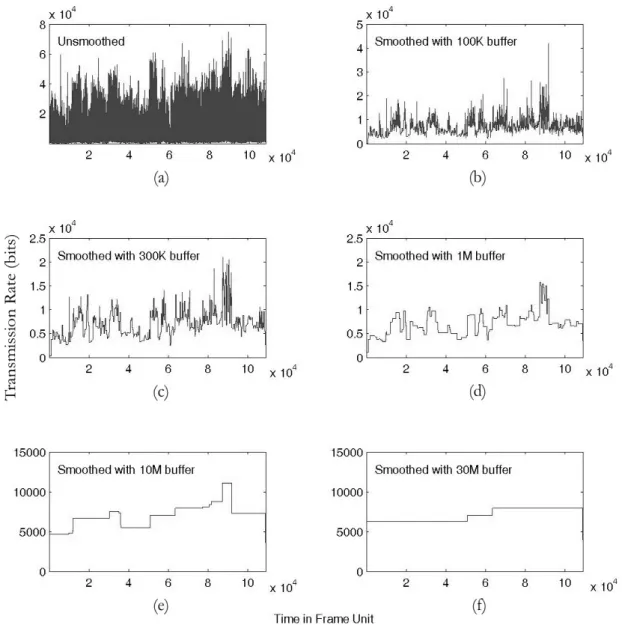
The following Fig. 8 is an illustration of the transmission schedules generated by MVBA with different client buffer size. We perform MVBA with 100K, 300K, 1M, 10M, 30M bits client buffer respectively. As the client buffer increase, the variation of transmission schedule and the peak rate lower, and the schedule is more like CBR.
Figure 8: The transmission schedule yielded by MVBA with different client buffer. (a) is the original video trace. (b) (c) (d) (e) (f) is yielded by MVBA with 100K, 300K, 1M, 10M, 30M client buffer respectively.
Fig. 8(a) is the original video trace. The variation is extremely large, and the peak appear at about 90,000th frame slot. The amount of frame data is 9,345 bytes.
buffer size. 100K is about the 1.5 times as large as the peak rate. Fig. 9 (a) is the transmission rate from the 91000th frame slot to 92000th frame slot generated by MVBA with 100K bits client buffer. The peak rate is at about 91650th frame slot. Fig.9 (b) is the result generated in MVBA process. Where the two fine stair lines represent the transmission upper bound and lower bound and the bold line segments are the transmission schedule. At about 91650th frame slot, there is a succession of large data frame. It induces the rate increasing rapidly and results in the peak rate of transmission schedule.
Note that the peak rate of the transmission schedule is still at about 90,000th frame slot, but the amount is a little bit lower, and variation is reduced significantly. This phenomenon is more apparent as the client buffer increase. See Fig. 8 (c) and Fig. 8 (d) as examples, which are transmission schedules after MVBA smoothing with 300K and 1M client buffer respectively.
Cu mu lative D a ta Time Rate
Figure 9: Peak rate of transmission schedule generated by MVBA with 100K bits client buffer size. (a) is the transmission rate. (b) is the transmission schedule and Upper and lower bound.
When the client buffer increases to 10M, the rate changes for less times but the peak rate appear at about 90,000th frame slot, and when the client buffer increases to 30M, it changes for only two times, and the transmission schedule is almost CBR.
The statistical data including maximum rate, minimum rate, average rate, mean to maximum ratio, and variance is shown in the following Table.1.
Tabel.1: The statistical data of transmission schedule of “Aladdin” smoothed with different client buffer.
Original Video Trace Smoothed with 100K buffer Smoothed with 300K buffer Mean Rate (bits/frame) 6,994.8 6,994.8 6,994.8 Minimum Rate (bits/frame) 72 111.0 333.0 Maximum Rate (bits/frame) 74,760 42,030 20,964 Mean/Peak (BFF) 0.094 0.166 0.334 Variance (bits2/frame) 72,480,467 9,788,187 7,325,169 Coefficient of Variance 1.217 0.447 0.387 Smoothed with 1M buffer Smoothed with 100K buffer Smoothed with 300K buffer Mean Rate (bits/frame) 6,994.8 6,994.8 6,994.8 Minimum Rate (bits/frame) 1,109.9 4,651.8 6,336.4 Maximum Rate (bits/frame) 15,675 11,076 7,466.4 Mean/Peak (BFF) 0.446 0.632 0.880 Variance (bits2/frame) 5,317,863 1,974,558 564,841
In table 1, the mean rate is defined as total video data
total number of frames , and the maximum rate and minimum rate are the maximum and minimum values of the
generated transmission schedule. The variance is defined as
2 1 ( ) N i i s mean N = −
∑
, andthe coefficient of variance is defined as variance mean , which represents the relation between the standard deviation, which equals to the square root of variance, and mean rate. The coefficient of variance represents the rate variation to mean rate ratio. According to the statistical data of table.1, we can find that the smoothing algorithm won't affect the average data rate. But the minimum rate will increase, and the maximum rate, variation, and coefficient of variation will decrease as the client buffer increase. The coefficient of variance of the unsmoothed transmission schedule equals to 1.217, it means that the mean variation of transmission rate is about 1.2 times of mean rate. When the client buffer is 30Mbits, the value equals 0.107, it means that the variation of transmission rate is only about 10% of the mean rate, and the transmission rate is vary close to CBR.
The mean to peak ratio is so-called bandwidth fill factor (BFF), which represents the efficiency of CBR channel usage. In CBR transmission, the requirement of bandwidth is the same as the peak rate of the data stream. Thus, the total data could be transmitted in this channel is Peak_rate N× , where N is the total frame number, and actually, the total transmitted data is
1 N i i a =
∑
. Then, the efficiency of usage of this channel is 1 1 1 _ _ _ _ N N i i i i a a Average rate N BFFPeak rate N Peak rate Peak rate
= =
= = = ×
∑
∑
When this factor equal to 1, it means the data rate is CBR, and as the client buffer increasing, BFF will more approach 1.
Fig. 10 is the illustration of the transmission schedule of different video traces which are yielded by MVBA with 1Mbits client buffer. (a) is "Terminator One" (b) is "Jurassic Park One" (c) is a video of baseball game. The same, the rate variation of transmission schedules is lowered.
Figure 10: Three transmission schedules of (a) Terminator One, (b) Jurassic Park One, (c) Baseball game, which are yield by MVBA with 1Mbit client buffer. Where the gray
The following Fig. 11 illustrates the effect of MVBA on the factors, peak rate, variance in transmission rate and BFF. It shows these factors as a function of client buffer. When the buffer client is very small, the transmission schedule is close to the unsmoothed schedule. As the client buffer increasing, the variance of rate and peak rate will decrease, the BFF will increase, and the transmission rate is more close to CBR.
4. Packet based Smoothing Algorithm
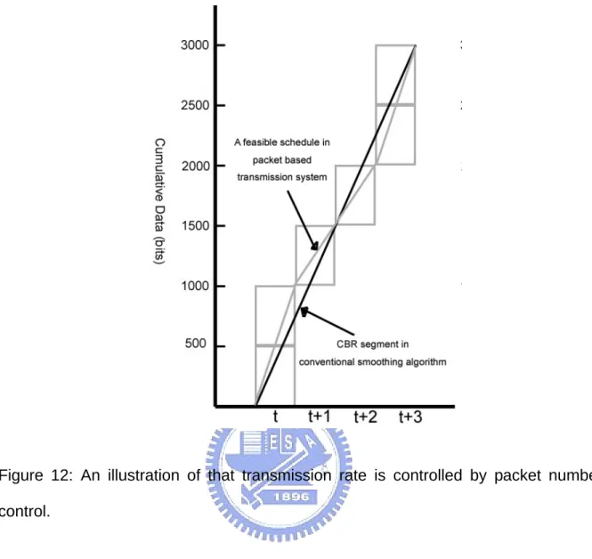
In most video streaming system framework, video data is packetized after being compressed, and then transmitted packet by packet in each frame slot. Therefore, transmission rate can only be controlled by transmitted number of packets in such system, but can't be controlled precisely according to MVBA schedule. See Fig. 12 as an example of this problem. In the example of Fig. 12, there are 3000 bits data waiting to be transmitted at 4 frame slots, these data are segmented into packets, which are in a size of 500 bits, and the rate of a CBR segment generated by certain conventional smoothing algorithm, such as MVBA, which we mentioned in Chapter 2, equals to 750 bits per frame slot. In Fig. 12, the black segment represents the CBR segment, but this CBR segment cannot be implemented in this case, because the server can only transmit data in a unit of packet, the transmission rate can only be the multiple of 500 bits. In this example, the server transmits two packets at t frame slot, one packet at t+1 and t+2 frame slots, and two packets at t+3 frame slot and the rate is 1000 bits per frame slot at t and t+3 frame slots and 500 bits per frame slot at t+1 and t+2 frame slot. The gray squares are the packet transmitted at the corresponding frame slot, and the gray segments represent the transmission schedule. This schedule can be implemented in the packet based transmission system but isn’t an optimum one.
Figure 12: An illustration of that transmission rate is controlled by packet number control.
Under this condition, the transmission schedule generated by conventional smoothing algorithm, such as we mentioned in chapter 2, cannot be used in the packet based transmission system, because the server can’t control the transmission rate precisely according to this schedule. In this chapter, we propose two methods for smoothing in packet based transmission system. These two algorithms can find the sub-optimum transmission schedule, which can be implemented in packet based
4.1 Number-of-Packets Based Smoothing Algorithm
In this section we describe the difference between Number-of-Packets Based Smoothing Algorithm and MVBA smoothing algorithm discussed previously, and demonstrate the relationship between transmitted packet number and transmission rate.
This algorithm aims to find a transmission schedule with a CBR packet rate. When the server transmitted the same number of packets at each frame slot, the transmission rate can be expected to be smooth. However, it’s similar to the MVBA smoothing algorithm described above. The finite client buffer makes the CBR transmission schedule of number of packets infeasible, only some piecewise-CBR schedules can obey the upper bound and lower bound. Thus, the transmission schedule generated by this algorithm will be with a more stable rate in transmitted number of packets, and the actual transmission rate is the sum of all packets transmitted at the corresponding frame slot. We will discuss the difference between the number-of-packets based smoothing algorithm and MVBA.
4.1.1 Modification of Upper Bound in Packet Based Smoothing Algorithm
Because the server transmits video data in a unit of packet, the transmission rate can’t be controlled arbitrarily. This fact induce that the client buffer can’t be utilized completely, therefore the upper bound of the two packet based smoothing algorithm have to be modified.
In packet based smoothing algorithm, the transmission data is restricted in unit of packet. Therefore a server can only transmit the video data packet-by-packet, the data that can be transmitted ahead to client buffer will be restricted and it induces client buffer not to be utilized fully. See the following Fig. 13 as an example. In Fig. 13, at the first frame slot, the server only can transmit the first six packets. If the client receives the seventh packet at the first frame slot, its buffer will overflow, and so will the buffer at second and third frame slot. Therefore, the upper bound will be modified to the level of the sum of the first six packets data at the first three frame slots. The upper bound at each frame slot will be modified in this way. The lower bound is the same with MVBA, because even the frame data is cut into packet, the sum of the packets data of a certain frame equals to its frame data.
Time Cumula tiv e Da ta
Figure 13: The difference of upper bound and lower bound between conventional smoothing algorithm and packet based smoothing algorithm. Where the black bold line represents the upper bound and lower bound in conventional smoothing algorithm, gray squares are data packets, and the gray line is the upper bound in packet based smoothing algorithm.
Next, the upper bound and lower bound are represented in packet number. See the following Fig.14.
Time Pack et N u mber
Figure 14: The upper bound and lower bound represented in number-of-packets form in packet based smoothing algorithm. We only consider the number of packets. ( )L k and ( )U k here is in unit of number of packets and represents the corresponding upper bound and lower bound in the previous figure.
In Fig. 14, the amount of data of each packet is ignored, and only the packet number is concerned, because we only care if the transmitted number of packets stays within the upper bound and lower bound. The server has to transmit until 2th
packet number at least and transmits until 6th packet number at most at the first frame
slot.
Thus, the lower bound in packet based smoothing algorithm is the total number of packets of previous frame slots,
where pi is the number of packets of frame i, and upper bound equals to the lower bound plus the number of packets, which can be preserved in client buffer at ith frame slot.
= +
'( ) '( ) i
U k L k b , (4-2)
where bi represents the number of packets which can be transmitted ahead at ith
frame slot. Take Fig.14 as an example, b1 equals to 4, because at this frame slot, the
client buffer can contain up to the sixth packet, and the client will consume the first two packets, and b2 equals to 3, b3 equals to 2, and etc.
Let '( )S k to be a transmission schedule representing the number of packets transmitted during k frame slot.
= =
∑
1 '( ) ' k i i S k s , (4-3)where 's i is the transmitted number of packets at ith frame slot. If the schedule is
feasible, it has to be within upper bound and lower bound,
≤ ≤
'( ) '( ) '( )
L k S k U k (4-4)
If we don’t care the actual data of each packet in packet based transmission system, the modified upper bound and lower bound represented in amount of data form and upper bound and lower bound represented in number of packets form are equivalent. Thus the area enclosed by the upper bound and lower bound represented in amount of data form also equals to the area enclosed by upper bound and lower bound in number of packets form. Therefore, a transmission schedule, which stays within a set of upper bound and lower bound must stays within the other set of upper
bound and lower bound as well. So a feasible schedule generated by packet based smoothing, which stays in the area enclosed by the upper bound and lower bound in number of packets form is also a feasible schedule and will stay in the area enclosed by the upper bound and lower bound in amount of data form.
4.1.2 Modification of integer transmission rate
The transmitted number of packets at each frame slot needs to be integer in a transmission schedule, which is generated by packet based smoothing algorithm. However, the rate generated by MVBA is unnecessarily to be integer. So we have to make the integer modification.
The transmission rate of an MVBA optimum schedule equals to smaxa b, or smina b,
in MVBA procedure. Therefore, calculation of smaxa b, and smina b, in
Number-of-Packets Based Smoothing Algorithm has to be modified as the following Fig. 15.
Time
Time
(a) (b)
Figure 15: The modification of integer transmission rate. (a) is a condition of
,
maxa b
s . In
order to prevent buffer overflowing,
,
maxa b'
s in Number-of-Packets Based Smoothing Algorithm takes the integer portion of
,
maxa b
s , and truncates the decimal part. (b) is a condition of
,
mina b
s . In order to prevent buffer underflowing,
,
mina b '
s rounds to the
nearest next integer of
,
mina b
s .
When smaxa b, is not an integer, smaxa b, ', the integer modified maximum rate in
Number-of-Packets Based Smoothing Algorithm, must be smaller than the original
,
maxa b
s , because
,
maxa b
s is the maximum feasible CBR transmission rate for all CBR segment in interval [ , ]a b . Thus the integer modification of
,
maxa b'
, max 1 ( ) ( ( ) ) '
min
a b a t b U t L a q s t a + ≤ ≤ − + ⎢ ⎥ = ⎢⎣ − ⎥⎦, (4-5)Similarly, the integer modified minimum rate in Number-of-Packets Based Smoothing Algorithm,
,
mina b'
s , must be larger than
, mina b s . That is a,b min a+1 t b L(t) - (L(a) + q) s ' = t - a
max
≤ ≤ ⎡ ⎤ ⎢ ⎥ ⎢ ⎥, (4-6)where ⎢ ⎥⎣ ⎦ is the floor function, ⎢ ⎥⎣ ⎦x returns the integer part of x, and ⎡ ⎤⎢ ⎥ is the ceiling function, ⎡ ⎤⎢ ⎥x returns the next nearest integer of x.
Thus, , maxa b' s and , mina b '
s are guaranteed to be integer, and the transmission schedule must stay within the upper bound and lower bound. So, the transmission schedule generated by Number-of-Packets Based Smoothing Algorithm is feasible, and the packet rate is integer for each frame slot.
4.1.3 The procedure of Number-of-Packets based smoothing algorithm
The initial settings of this algorithm are the same as the MVBA, and the process starts from the beginning of the video. After the upper bound and lower bound is calculated, these upper bound and lower bound will be modified to the number-of-packet form, as Fig. 14. Then the process will calculate the
, mina b s , , maxa b s ,
underflowing condition happens or not, which are described in section 2.1.2. Then the reaction is the same as MVBA. The process will repeat until the total video is be segmented. Finally, the sum of the data of the corresponding number of packets is the actual transmission rate.
4.2 Packet Mapped Smoothing Algorithm
This algorithm is to find a suboptimal transmission schedule, which approximate the optimum schedule generated by MVBA as well as possible, in packet based transmission system. We describe how transmission rate could be controlled to approximate to the optimal schedule generated by MVBA and stay within the feasible area by control of transmitted number of packets.
4.2.1 Upper and Lower Bound in Optimum Transmission Schedule
In MVBA algorithm,
,
maxa b
s is the maximum feasible transmission rate in interval [a,b]. If the total transmitted data is above line segment,
,
maxa b
s , the client buffer may be overflowing within this interval. Therefore, when MVBA decided to transmit in rate
,
maxa b
s in interval [a,b], the total transmitted data can't be above line segment smaxa b, ,
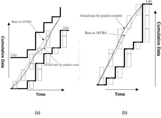
as the following Fig.16(a). The two block bold lines represent the upper bound, U(k), and lower bound, L(k). The gray squares under L(k) is the data packet at the corresponding frame slot. Gray line segment is the optimum transmission rate decided by MVBA in this interval. Black fine line segments are the transmission rate controlled by transmitted number of packets, and the gray squares between upper
bound and lower bound are the packet transmitted at the corresponding frame slot. In Fig.16(a), if server transmits the next packet, which is transmitted at 4th frame slot, at 3rd frame slot, the total transmitted data will be above line segment smaxa b, , and it
results in buffer overflowing. Thus the sum of the transmitted data can’t be above
,
maxa b
s , when MVBA decide to transmitted with rate
, maxa b s in interval [a,b]. Time Cumulativ e Dat a Time Cumula tiv e Da ta
(a) (b)
Figure 16: Number of packets controlled rate control. (a) represents the condition that the optimum schedule is
,
maxa b
s . The total transmitted data can't be above the line segment
,
maxa b
Similarly,
,
mina b
s is the minimum feasible rate in MVBA, if the total transmitted data is below line segment
,
mina b
s , the client buffer may be underflowing within this interval. Therefore, when MVBA decided to transmitted in rate
,
mina b
s in interval [a,b], the total transmitted data can't be below line segment
,
mina b
s , as Fig.16(b).
4.2.2 The procedure of Packet Mapped smoothing algorithm
The packet mapped smoothing algorithm performs original MVBA with the modified upper bound and lower bound in amount of data form, and then calculate the packet number that the cumulative data from the end of the previous frame to this calculated packet number is nearest to the optimum transmission schedule, which is generated by MVBA, with obeying the two principles described above. By this way, the transmission schedule will approximate to optimum schedule of MVBA and be feasible.
4.3 Implementation of Packet Based Smoothing Algorithm
To transmit smoothly without modifying video stream standard is the greatest benefit of packet based smoothing algorithm. Take MPEG4 as an example, after encoder compresses the video data, the compressed data will be cut into packets and be transmitted on the network. The encoder will mark the quantization coefficients, the frame number and other parameters in the packet header. Then the client
reassembles these packets and decodes frame data according to the header of packets. However, the optimum transmission schedule generated by MVBA won't match the data packets exactly. If the server would like to follow the optimum transmission schedule completely, the data packets have to be segmented again. Thus, there must be a mechanism, which reassembles these new packets in client. Otherwise, these packets can't be decoded correctly. But, this mechanism does not conform to the standard. So, the packet based smoothing algorithm can make the clients conform the video compression standard, moreover, it can make network to be utilize efficiently.
The token bucket algorithm can control the amount of data, which are inserted into the network. It’s a transmission mechanism that determines when the traffic can be transmitted, based on the presence of tokens, and the bucket leaks a variable number of token periodically. The server can control the period. Then the streamer will transmitted the same number of packets according to the leaked number of tokens. We can implement our algorithm easily by using this token bucket algorithm. In our system, we insert a token bucket between the encoder and network layer. After the video is compressed, the data will be packetized and this packet will be stored in a buffer in packet order. The token bucket leaks some tokens according to the transmission schedule generated by our packet based smoothing algorithm. Then the streamer releases the same amount packets. Therefore, our smoothing algorithm can control the transmission rate. Fig. 17 shows this mechanism.
Leaked Bucket
Figure 17: Block diagram of a video transmission server with packet based smoothing algorithm.
5. Simulation of Packet Based Smoothing Algorithm
In this chapter, we also use the video trace "Aladdin" to demonstrate examples of Number-of-Packets Based Smoothing Algorithm and packet mapped MVBA. This video trace is in QCIF format, 30 frames per seconds, and compressed with MPEG4 and with I-P-B quantization level 10-14-16. We perform these two algorithms with four different maximum packet sizes, 512 bits, 1024 bits, 1536 bits and 2048 bits and observe the statistical parameters of simulation result to compare with the original MVBA algorithm.
5.1 Performance of Number-of-Packets Based Smoothing
Algorithm
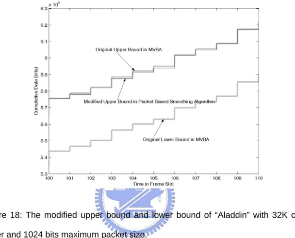
At the first of the packet based smoothing algorithm, the upper bound has to be modified. The procedure will find the packet number, until which the cumulative data is nearest to the original upper bound but isn’t above it. By this way, the upper bound and lower bound in number of packets form are generated. Then the upper bound in packet based smoothing is modified to the cumulative data until the corresponding packet number for each frame. Thus, the modified upper bound and lower bound in amount of data form are found. Fig. 18 and Fig. 19 are the modified upper bound and lower bound of the 100th to 110th frames of video “Aladdin” in packet based
the original upper bound in MVBA and the modified upper bound in packet based smoothing algorithm.
Figure 18: The modified upper bound and lower bound of “Aladdin” with 32K client buffer and 1024 bits maximum packet size.
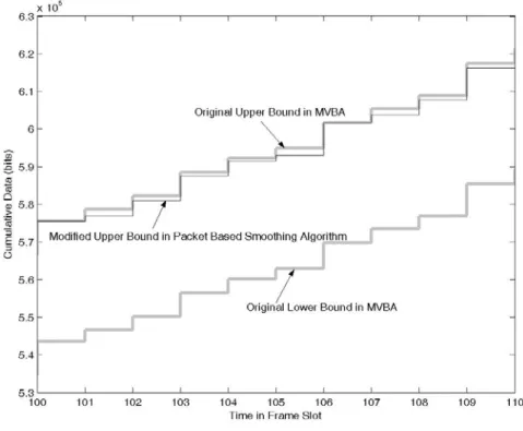
Figure 19: The modified upper bound and lower bound of “Aladdin” with 32K client buffer and 2048 bits maximum packet size.
Then the procedure performs the integer modified MVBA algorithm on the modified upper bound and lower bound in number of packets form to find the transmission schedule of number of packets. Fig. 20 and Fig. 21 are the examples of the transmission schedule of video “Aladdin” with 32K bits client buffer and 1024 bits maximum packet size and 2048 bits maximum packet size respectively. It shows that the number of packets with 1024 bits maximum packet size is about twice as the packet number with 2048 bits maximum packet size at the same frame slot, because the number of packets with 1024 bits maximum packet size is about twice as the
with different maximum packet size, the transmission schedule of number of packets are also quite different.
After the transmission schedule of number of packets is generated, we sum the corresponding number of packets for each frame to calculate the actual transmission rate. Fig. 22 and Fig. 23 are the two results. Compare Fig. 20, Fig. 21 and Fig. 22, Fig. 23, it is apparent that although the server transmits the same number of packets, the actual rate varies because the size of the successive packet may be different.
Figure 20: Transmission schedule of number of packets of “Aladdin” with 32K bits client buffer and 1024 bits maximum packet size.
Figure 21: Transmission schedule of number of packets of “Aladdin” with 32K bits client buffer and 2048 bits maximum packet size.
Figure 23: Transmission schedule of actual data rate of “Aladdin” with 32K bits client buffer and 2048 bits maximum packet size.
The following Fig. 24 and Fig. 25 are the transmission rate of the schedule generated by Number-of-Packets Based Smoothing Algorithm with 32K bit client buffer and 1024 bits and 2048 bits maximum packet size respectively. Fig. 24 (a) and Fig. 25 (a) is the number of packets transmitted at each frame slot, and Fig. 24 (b) and Fig. 25 (b) is the actual transmission rate at each frame slot.
Figure 24: Transmission rate of the first 1000 frames of “Aladdin” generated by Number-of-Packets Based Smoothing Algorithm with 32k bits client buffer and 1024 bits maximum packet size. (a) is the number of packet transmitted at each frame slot. (b) is the actual transmission rate.
Figure 25: Transmission rate of the first 1000 frames of “Aladdin” generated by Number-of-Packets Based Smoothing Algorithm with 32k bits client buffer and 2048 bits maximum packet size. (a) is the number of packet transmitted at each frame slot. (b) is the actual transmission rate.
The following Fig. 26 and Fig. 27 are the transmission rate of the total video “Aladdin” generated by Number-of-Packets Based Smoothing Algorithm with 100k bits and 1M bits client buffer size respectively and maximum packet size 1024 bits, and Fig. 28 and Fig. 29 are with 100k bits and 1M bits client buffer size respectively and maximum packet size 2048 bits. Where (a) is the number of packets transmitted at each frame slot, and (b) is the actual transmission rate.
Figure 26: The transmission rate of the total video “Aladdin” generated by Number-of-Packets Based Smoothing Algorithm with 100k bits client buffer and 1024 bits maximum packet size. (a) is the transmission Number of packets at each frame slot. (b) is the actual transmission rate.
Figure 27: The transmission rate of the total video “Aladdin” generated by Number-of-Packets Based Smoothing Algorithm with 1M bits client buffer and 1024 bits maximum packet size. (a) is the transmission Number of packets at each frame slot. (b) is the actual transmission rate.
Figure 28: The transmission rate of the total video “Aladdin” generated by Number-of-Packets Based Smoothing Algorithm with 100k bits client buffer and 2048 bits maximum packet size. (a) is the transmission Number of packets at each frame slot. (b) is the actual transmission rate.
Figure 29: The transmission rate of the total video “Aladdin” generated by Number-of-Packets Based Smoothing Algorithm with 1M bits client buffer and 2048 bits maximum packet size. (a) is the transmission Number of packets at each frame slot. (b) is the actual transmission rate.
According to these examples, it’s obviously that even though the number of packets transmitted at each frame slot is smoothed, the actual transmission rate is still with much variation because of the size difference between successive packets. For example, at B frame duration or at the time of static scene of a video, there may be more small packets, and at I frame duration or at the time of scene with high motion components, there will be more full packets. Thus, even the transmitted number of packets is the same, the actual transmission rate, which equals to the sum of the
successive packet data, will be different. The variance of transmitted number of packets will tend to decrease as the client buffer increasing, and the actual transmission rate will vary in accordance with the variation of transmitted number of packets and the data variation between the succession packets. Therefore, the transmission rate with larger maximum packet size may tend to be with more variation, because the larger the maximum packet size is, the more the difference between successions packets can be. It’s also shows that the transmitted number of packets will be influenced by the integer rate modification. The integer rate modification may induce the transmitted number of packets varying between two adjacent integers.
Because of the two uncertain factors, the transmitted number of packet and the difference size between successive packets, it’s hard to predict the performance of Number-of-Packets Based Smoothing Algorithm with different client buffer and different maximum packet size. The larger client buffer may lower down the variation of transmitted number of packets, but the integer rate modification may make the transmitted number of packets varying more times between two adjacent integers with certain maximum packet size. The larger maximum packet size will induce the more variation between the successive packets, but the different maximum packet size will also yield different upper bound of number of packets. The different upper bound and lower bound will generate different transmission schedule. Therefore, we only can confirm that the Number-of-Packets Based Smoothing Algorithm with smaller maximum packet size and large client buffer size may tend to generate a schedule with lower variance in transmission rate in a high probability, but it also may generate