流動性危機與銀行資本適足率策略探討─以歐債危機為例 - 政大學術集成

全文

(1)國立政治大學國際經營與貿易學系碩士論文 Rethinking on Liquidity Shock and Capital. 治. 政under European Requirement Strategies Debt Crisis 大. 立. ‧ 國. 學. 流動性危機與銀行資本適足率策略探討以歐債危機為例. ‧. n. er. io. sit. y. Nat. al. Ch. engchi. i n U. v. 指導教授：胡聯國博士研究生：周均亭. 中華民國一百零一年六月.

(2) 摘要銀行資本適足率為確保整個銀行與經濟體系穩定與完善的重要指標之一，而近年來隨著新巴塞爾協定之推行，經濟學家間掀起關於現行資本適足率的適切性的討論。本篇論文以流動性危機、道德風險建構模型，在此基礎下推導出最適資本適足率策略，模型主要論點為資本適足率需根據各國經濟情勢而有所調整，當一國的 GDP 與利率呈現正向關係時，意味資本適足於經濟成長時緊縮(提高)，而於經濟衰退時放寬(下降)；而當一國 GDP 與利率呈現負相關時，則資本適足率. 政治大. 於經濟成長時放寬(下降)，而於經濟衰退時緊縮(提升)。. 立. 在此模型理論基礎下，本篇論文以歐元區十七國之資料來深入探討歐債危. ‧ 國. 學. 機之下資本適足率的策略。實證結果顯示，在 2005Q2 到 2011Q3 大部份的國家 GDP 與利率呈現正向關係，亦即資本適足率與所得之反向循環策略是較適當的，. ‧. 追蹤資料分析更指出貿易程度開放的國家需要相對較嚴格的資本適足率策略，而. y. Nat. sit. 較傾向實行財政政策之國家需要更寬鬆的資本適足率策略。本篇論文亦對 2012. n. al. er. io. 年各國應有的資本適足率策略做預測，結果證實歐洲各國應採行資本適足率與所. i n U. v. 得之正向循環策略，其中，希臘、義大利、西班牙、法國，在經濟衰退之時需要. Ch. engchi. 寬鬆的資本適足率策略，但寬鬆(下降)幅度必需有所限制。. 關鍵字：資本適足率、歐債危機、巴賽爾協定、流動性危機. i.

(3) Abstract Capital requirement serve as an important key for ensuring the stability and effectiveness of the overall economy. As the new Basel Accord has announced, debates over how capital requirement should be implemented, especially in the times of crisis, are heated among economist. In this paper, based on liquidity shock and moral hazard problem, we derive the optimal capital requirement strategies, which depend on general economic condition. We argue that counter-cyclical capital. 政治大. requirement, which adopts looser capital requirement when GDP decreases and. 立. increases capital requirement when GDP increases, should be adopted when GDP and. ‧ 國. 學. interest rate is positively correlated while pro-cyclical capital requirement are appropriate when GDP and interest rate is negatively related.. ‧. To further characterize the problem under European Debt Crisis, we use 17. y. Nat. io. sit. countries in Euro Zone to conduct empirical test and panel estimation. We conclude. n. al. er. that most countries should adopt counter-cyclical capital requirement during 2005Q2. i n U. v. to 2011Q3. Besides, our panel estimation indicate that countries with more trade. Ch. engchi. openness should adopt more flexible capital requirement policies, while countries who focus more on fiscal policy weight should have larger adjustment on their capital requirement. Finally, our forecast result suggests that in 2012, all the countries in Euro Zone should adopt counter-cyclical capital requirement policies. In particular, Greece, Italy, Spain, Portugal and France should have looser capital requirement compared to other countries. Keywords: Capital Requirement, European Sovereign Debt Crisis, The Basel Accord, Liquidity shock. ii.

(4) 謝辭回想兩年前毅然決然決定從外語學院踏入商學研究所，當時很不確定如此抉擇是否正確，如今看來完全沒有後悔的理由，這兩年在系上教授與政大其他系所優異的師資指導之下，我獲得與原本學習領域完全不同的思考方式，對我來說，是感動、是震撼，也是滿滿的感謝。怎麼也想不到自己能擁有如此充實的研究所生活，並且能在這段學習時光結束的尾聲，順利的完成我的碩士論文。在此，我最要感謝的是我的指導教授胡聯國博士，胡老師的知識領域既廣. 政治大的學識大有精進，胡老師的人文風範也是我的楷模，時時提醒著我不要忘記商學立. 又精，在做論文的過程中給予我相當多的指導，不僅在論文，也讓我對相關領域. ‧ 國. 學. 需要人文素養的相輔相成。非常感謝胡老師在忙碌之餘，還盡心盡力的指導我，讓本篇論文能夠順利的完成，在此向胡老師致上最深的感謝之意。非常感謝林柏. ‧. 生博士與龔尚智博士在百忙之餘抽空參與我的論文口試，並且給予最精闢的建議，. sit. y. Nat. 彌補本篇論文的不足之處。林老師對於數理模型的建構與掌握、龔老師對於邏輯. al. er. io. 的推演，在在令我佩服不已。. v. n. 感謝我的家人在念研所的時期無時無刻在經濟上以及心理上支持我，讓我能. Ch. engchi. i n U. 夠無後顧之憂專心在理論與實務的精進上，並且能夠在工作之前有一段能夠放心的踏上尋找自我的交換學生之旅，就此，我感到自己無比幸運。感謝在研所這段時間所有給我鼓勵、與我合作的國貿所同學，從你們身上我得到許多，相信如果少了你們我的研所生活會暗淡不少，我想特別感謝我的研究所同窗兼論文戰友蕭筑方，陪我一起度過這段非常忙碌時期，也給予我很多幫助，因為有妳的陪伴，許多困難都迎刃而解，我想我以後會很想念我們一起努力達成目標的時光。卻顧所來徑，我得之於人者太多，付出卻還嫌太少。未來我期許自己能夠擁有一顆體諒他人的心，不要忘記自己必須為家人朋友、還有社會上需要幫助的人盡一份心力，勿以善小而不為，如此才不枉這些年之所學。 iii.

(5) CONTENTS. 摘要 ....................................................................................................................................... i Abstract ................................................................................................................................ ii 1.. Introduction .................................................................................................................. 1 1.1. European Sovereign Debt Crisis ........................................................................... 1. 1.2. Basel Accord and Capital Requirement ................................................................ 2. 2.. Literature Review .......................................................................................................... 5. 3. The Model ................................................................................................................... 10. 3.3. Bankruptcy Threshold from Consumer's Approach .......................................... 14. 政治大. Optimal Capital Requirement ...................................................................................... 17. 立. 4.1. GDP and Interest Rate ........................................................................................ 17. 4.2. Keynesian Model and the Specific Form ............................................................ 19. The Estimation and Result ........................................................................................... 22 The Data .............................................................................................................. 22. 5.2. Simple Regression ............................................................................................... 22. 5.3. The Result ............................................................................................................ 25. ‧. 5.1. y. sit. Panel Data Estimation .................................................................................................. 29 The Unit Root Test............................................................................................... 29. 6.2. Panel Data Analysis ............................................................................................. 30. 6.3. Forecasting and Future Policy Suggestion .......................................................... 33. er. 6.1. io. al. v i n Ch Conclusion .................................................................................................................. 36 engchi U n. 7. Loan-Equity Ratio and Bankruptcy Threshold .................................................. 11. Nat. 6. 3.2. 學. 5. The Set Up ........................................................................................................... 10. ‧ 國. 4. 3.1. Appendix A: Detail Definition of Variables ............................................................................ 38 Appendix B: Value of Interest-Rate-to-Income Effect in 17 Euro Zone Country ....................... 41 Appendix C: Descriptive Analysis of Raw Data ...................................................................... 43 C.1 GDP . ............................................................................................................................ 43 C.2 Cumulative Debt Level to GDP ratio .............................................................................. 44 C.3 Trade Openness (Trade flow/GDP) ................................................................................. 46 C.4 Monetary and Fiscal Policy: Weight and Effectiveness .................................................. 48 Reference ............................................................................................................................ 52. iv.

(6) LIST OF FIGURES. Figure1 Trend of Interest- Rate-Change-to-Income Effect for PIIGS .................................................. 27 Figure2 Trend of Interest- Rate-Change-to-Income Effect for Relatively Small Variation .................. 27 Figure3 Trend of Interest- Rate-Change-to-Income Effect for Relatively large Variation ................... 28 Figure4 Forecast of 2012 Interest-Rate-Change-to-Income-Effect Before First differencing .............. 35 Figure5 Forecast of 2012 Interest-Rate-Change-to-Income-Effect After First differencing ................ 35 Figure6 GDP for Main 17 Euro Zone Countries (Unit: Millions of Euro) ........................................... 44 Figure7 Cumulative debt/GDP in Greece, Ireland, Spain, Italy and Portugal ...................................... 45 Figure8 Cumulative Debt/GDP in Other Major Euro Zone countries .................................................. 45 Figure9 Trade Openness in Greece, Ireland, Spain, Italy and Portugal ................................................ 47. 政治大. Figure10. Trade Openness in Other Major Euro Zone countries ......................................................... 47. Figure11. Fiscal Policy Weight for PIIGS (Unit: Percentage Rate %) ................................................. 49. Figure12. Fiscal Policy Weight for Other Major Countries (Unit: Percentage Rate %) ...................... 49. Figure13. Fiscal Policy Effectiveness for Major 11 Euro Zone Countries .......................................... 51. Figure14. Monetary Policy Effectiveness for Major 11 Euro Zone Countries .................................... 51. 立. ‧. ‧ 國. 學. n. er. io. sit. y. Nat. al. Ch. engchi. v. i n U. v.

(7) LIST OF TABLES. Table1 Simple Regressions Results on. . ............................................................ 24. Table2 Unit Root Test Result for variables in (6.1) .............................................................................. 30 Table3 Panel Estimation Result for Variables in (6.1) Before First differencing ................................. 32 Table4 Panel Estimation Result for Variables in (6.1) After First differencing .................................... 32. 立. 政治大. ‧. ‧ 國. 學. n. er. io. sit. y. Nat. al. Ch. engchi. vi. i n U. v.

(8) 1. Introduction 1.1 European Sovereign Debt Crisis European sovereign debt crisis is an ongoing crisis. The causes can be roughly attributed to international trade imbalance, easy access to borrowing money, bailout spending in financial crisis in 2008, and the further economic recessions from 2008 to 2012. Relative to Germany, Greece, Ireland, Portugal, Italy and Spain has large amount of trade deficit. The trade imbalance has kept worsening, thus resulting series. 政治大. fiscal deficit. Besides, increase savings around globe during 2000 to 2007 made the. 立. money available for investment, as investors seeking for higher yields target than US. ‧ 國. 學. treasury bonds. Increase investment in fixed income securities, together with the guarantee of Euro Zone, has made Greece and Ireland get easy access to borrow. ‧. money. After the bubble burst and the asset price declined, the liability owned to. y. Nat. io. sit. global investors remains at full price, thus deepening government’s debt burden.. n. al. er. Finally, the bailout spending during financial crisis has been the last straw. The bailout. i n U. v. package has transformed the debt from private sector, such as banks, to the. Ch. engchi. government. With the high debt levels and low existing interest rate, the government is left with few policies to take over the burden. In 2008, Greek government’s bond yield rises from 25 basis point to 65 basis point, reflecting the starting point of investors demanding high interest rate from governments with higher debt and high deficit levels. These governments have a hard time financing its existing debt and deficit. The subsequent downgrading of credit risk in Greece, Ireland and Portugal, accompanied by the rising government debt exceeding its GDP ratio in these countries, has aroused tremendous fears among investors. In 2010, the worries are intensified when the market found out the Greek’s 1.

(9) deficit is much worse than it claimed. To restore confidence of Europe as well as ensuring financial stability across Europe, EU creates a European Financial Stability Facility (EFSF)1. IMF and the Euro Zone agree to bailout Greece, following later Portugal and Ireland. The bailout is at the cost of the promise that the government will cut its spending budget and start debt reconstruction plan. Soon after, Greece starts to unveil a series of austerity measures2 aim at cutting the deficit. However, the excessive spending cuts bring Greece into serious recession. In 2012, the subsequent bailout plan has been agreed by EU. However, the opposition voice against austerity. 政治大 Italy, and the economic contraction has been reported across Europe, it seems the 立. measure has spread among Euro Zone. With debt borrowing kept rising in Spain and. Europe sovereign debt is just at its beginning.. ‧ 國. 學. In this paper, we look at the capital requirement policy to examine the current. ‧. response to European sovereign debt crisis. We use data in 17 countries in Euro Zone. sit. y. Nat. to find suitable capital requirement strategies. We also discuss whether current. io. er. austerity measure, especially capital requirement policy, is capable of solving the crisis. But first, we will give a brief review on now-existing Basel Accord and capital. n. al. requirement.. Ch. engchi. i n U. v. 1.2 Basel Accord and Capital Requirement The Basel Accord, conducted by the Basel Committee on Banking Supervision (BCBS) to set a standard of capital requirement in banks all over the world, has become an important regulation to prevent international risk and crisis. It is the most crucial banking supervision standard in the world. The goal of Basel Accord has been. 1. ESFS serve as special vehicle financed by members in Euro Zone to address European debt crisis, with the objective to provide financial support to Euro Zone states in economic difficulty. It was set on 9, May, 2010. The headquarters are in Luxemburg. 2 Austerity Measure refers to policies that involved with cutting the spending to lower the deficit. 2.

(10) insuring stable management as well as fair competitiveness among banks. Over the years, capital requirement policy has evolved substantially under the standards set by the Basel Committee on Banking Supervision (BCBS). In 1988, the Committee set a capital requirement standard that assets are grouped into five categories according to credit risk3, which refers to as Basel I. As the goal of Basel I is simply to raise capital requirement in some countries regarded low capital requirement level, Basel I has been criticized for making very limited distinctions through risk weights between difference in credit risk.. 政治大 characteristic is to make minimum capital standards more risk-sensitive, which is 立. Later in 2004, the Committee agreed on a new capital framework whose fundamental. refers to as Basel II. The capital charges of Basel II are based on asset quality rather. ‧ 國. 學. than on asset type. It will permit banks to use its own internal rating system (IRB) to. ‧. quantify the creditworthiness of their debtors. As in the old framework, total capital. sit. y. Nat. requirement are still 8 percent of risk-weighted asset. Besides, Basel II has. io. er. strengthened the ability of supervisors to require higher capital targets above the minima based on an assessment of risk management. It also develops more. al. n. v i n C h to allow the market transparency disclosure requirements participants to judge the engchi U capital requirements of an institution.. However, the common criticism for Basel II is. the regulation often incur procyclicality problem4. Skeptics believe that requiring bank to hold more capital requirement when banks are exposed to greater risk will further induce economic downturn, or bankruptcy. After the financial crisis in 2008, the Committee once again revises the capital requirement standard as Basel III. Besides strengthening risk coverage, new 3. The five asset categories are risk weights of zero (mostly home sovereign debt), ten, twenty, fifty and one hundred percent (mostly corporate debt). 4 Basel II Accord require bank to raise their capital requirement when they face more risk, so bank will lend less during recessions. The contraction will further make the economic condition worse. On the contrary, less capital requirement holding in the boom will is likely to create bubbles. 3.

(11) regulatory requirements on bank liquidity and bank leverage were introduced. A minimum of 3% leverage ratio is required, and bank should hold sufficient high-quality liquid asset. These changes are aim to enhance risk-management, reduce procyclicality as well as promoting countercyclicality, avoid moral hazard problem, and increase transparency. From Basel I to Basel III, the Committee has been dedicated on setting capital requirement that ensures bank be able to withstand crisis as well as maintain its stability. However, whether the new capital requirement will be appropriate for each country is still under debate.. 政治大 in which deposit and equity capital level are only depends on the decision of a 立. In this paper, follow the framework of Len-Kuo Hu (2012), we considers a model. representative, who simultaneously plays three roles including a representative. ‧ 國. 學. consumer, a depositor and the bank’s equity holder. Our main argument is capital. ‧. requirement should follow different strategies across different countries and times,. sit. y. Nat. according to its economic condition. More specifically, we suggest that when GDP is. io. er. negatively related to the interest rate, the country’s authorities should raise the required ratio in recession and lower it in the boom. On the contrary, the countries’. al. n. v i n Ch authorities should raise capital requirement in boom and lower it in recession if the engchi U GDP is positively related to interest rate.. The rest of the paper is organized as follows. Related Literatures concerning European debt crisis, liquidity shock and capital requirement are reviewed in section 2. A summary of liquidity shock model will be presented in section 3 and 4. Section 5 and 6 performs descriptive analysis and panel estimation to find out the appropriate capital requirement strategies under European debt crisis. Section 7 concludes our main argument and results.. 4.

(12) 2. Literature Review European sovereign debt crisis is an ongoing crisis, but the fundamentals of the crisis and the future impacts are still under debate. Arghyrou and Tsoulalas (2011) consider the European Sovereign debt crisis as a currency crisis. Using Obstfeld (1996) and currency model,5 they conclude that Greek debt crisis will continue to escalate because market expectation for Greece has shifted from credible commitment with implicit guarantee from Germany, to non-credible commitment without any backed. 政治大 Thus, they only way out for立 Greece is to rely on IMF's emergency financing, or leave. guarantee, making the cost of maintaining the currency peg higher than abandoning it.. ‧ 國. 學. the EU eventually.. Vitek and Bayoumi (2011) estimated a structural macroeconomic model of the. ‧. world economy to analyze possible future spillovers from real and financial shock. sit. y. Nat. mainly from Greece, Ireland and Portugal both within Euro area and to the rest of the. n. al. er. io. world. The result suggests macroeconomics and financial market spillovers have been. i n U. v. small to countries with high trade or financial exposures, but it will be of more. Ch. engchi. concern if Italy and Spain are under large financial pressure. Besides, they also find that monetary policy response produce limited scope to reduce the spillovers. It requires fiscal and financial policy measures to both alleviate market concern and respond to future large adverse shock in Euro Area member countries. One of the interesting findings by Reinhart and Rogoff (2010) are worthy of mentioning. They extended the debt data to a range of half a contrary, form 1980 to 5. The government balances the credibility cost incurring by defaulting on the exchange-rate peg commitment against the macroeconomic cost arising from deviating from the peg-maintenance. In the first generation model, excessive deterioration in fundamentals will result in the peg’s collapse since the cost of maintaining the peg exceeds defaulting. However, in the second generation model, which applies on Greek before the debt crisis, the peg’s cost is endogenous to the private sector’s expectations. Under credible commitment, overvaluation defending the peg is less costly. 5.

(13) 2009. One of their results indicate banking crisis always precede or accompany sovereign debt crisis6, which may explain the financial banking crisis in 2008 has indirectly b cause European sovereign debt cerise, and the debt crisis may further inducing another banking crisis. Due to the close relationship between debt crisis and banking crisis, we narrow down our research focus to the role banking regulation, specifically referring to capital requirement, during the time of debt crisis. Numerous papers have concerned the issue of capital requirement, showing its crucial roles in banking regulation and supervision. One particularly issue raised is the. 政治大 capital requirement during recession and loosing it during contraction will further 立. procyclicality of Basel I and Basel II, which is the debate over whether the raising. cause economic fluctuations. If the capital requirement increases in recessions, given. ‧ 國. 學. that raising capital is very costly, banks would have to reduce loans and the. ‧. subsequent credit crunch would deepen the downturn.. sit. y. Nat. Kashyep and Stein (2004) argue that under Basel II capital requirement, additional. io. er. procyclicality impact is significant. Their theory suggests that capital requirement should come down when the economy is in downturn, i.e. economy-wide bank capital. al. n. v i n C h They also propose is scarce relative to lending opportunities. that capital requirement engchi U rule should base on aggregate business cycle indicators, such as creating to GDP threshold.. Rabell, Jackson and Tsomoso (2005) find that more stable rating scheme. over the cycle would not further induce the procyclicality of capital requirement, whereas ratings according to the current point of the cycle would significantly increase procyclicality. However, bank will not choose the more stable rating system, meaning the procyclicality problem is still big issue. Heid (2007) prove under Basel I. 6. They use VAR method to test the relationship. Both variables, banking crisis and debt crisis dummies, are treated as endogenous, which can be explained by its own lagged values and the lagged values of the second variables. Their results also indicates that systematic banking crisis in financial centers help explain domestic banking crisis, which is very intuitive. 6.

(14) and Basel II, procyclicality problem exist, but can be mitigated by capital buffer 7. decisions. In addition, they point out the procyclicality effect will vary among. countries, depending on different macroeconomic fluctuations. Conversely, Zhu (2007) proposed a completely different view, stating that Basel II does not necessarily cause procyclicality of capital regulation, which he uses capital buffer to measure instead of the change in regulatory capital. The capital requirement does not affect the volatility of the bank credit and economic output. Furthermore, higher volatility of capital rule does not necessarily result in big movements in bank’s. 政治大. lending activity, since banks often choose loans that are different from that of the regulated capital constrains.. 立. Finally, two empirical tests conducted in Europe, which is the main focus of this. ‧ 國. 學. study, also have different results on the issue of procyclicality. Ayuso et al. (2004). ‧. indicates that instead of arguing the procyclicality of capital requirement, we should. sit. y. Nat. examine capital buffer's variation over business cycle. The reason is few banks hold. io. er. just capital requirement, while most keep capital buffers. They perform empirically test using Spanish data from 1986 to 2000. They confirmed that an increase of one. al. n. v i n C hcapital buffers by 17%, percentage in GDP growth reduces meaning that the test engchi U. support procyclicality of Basel II. However, similar empirical testing on Germany, conducted by Stolz and Wedow (2011) on the contrary indicates procyclicality of Basel II is not clear. Their results demonstrate a fundamental concern of this paper: Should capital requirement implement a certain formula in every country, regardless of the variation of economic situation across each country? As capital requirement can affect bank's liquidity decision, both in advance of. 7. Capital Buffer refers to the amount banks have to hold above minimum requirement, according the forecast of risk. There are two types of Capital buffer, capital conservation buffer and countercyclical buffer. The former focus on individual bank’s financial condition while the latter’s goal is more macro-prudential, which protects the banks form excessive credit growth. 7.

(15) credit extension as well as facing serious economic downturn, another issue we must address here is bank's liquidity. Diamond and Dybvig (1983) proposes that bank can transform illiquid asset into liquid demand deposits, but banks do not know the exact time of all depositors. If the liquidity needs of many depositors come at one time, or more seriously, the self-fulfilling runs8 occur, it may force bank to liquidate the illiquid asset in a wrong time, further jeopardize bank’s activity. Roche and Tirole (1996) also use their model to prove that in the optimal financial contract linking each bank and its lenders, the bank is subject to liquidity requirement, in proportional to its. 政治大 management by centralizing the payment system, the Fed funds markets, and other 立 risky asset. To prevent systematic risk, government should implement the liquidity. markets where banks are exposed to each other. This would ensure efficient liquidity. ‧ 國. 學. allocation among banks. As suggested by Borio and Zhu (2011), weak liquidity. ‧. constraint can support higher risk-taking, and effectively increase risk-tolerance. In. sit. y. Nat. turn, the greater risk-tolerance also relaxes external funding constraints. Whereas. io. er. when liquidity condition tightens, risk-tolerance and risk-taking ability decrease. Farhi and Tirole (2012) use a liquidity hoarding model to argue that when everyone. al. n. v i n take part in maturity mismatch ,C the optimal policy forU h e n g c h i the authority is simply to 9. bailout, which creates a social cost. To further discuss the choice of bailout policy, they propose that interest rate policy, including any measure that will lower financial institutions borrowing cost, is always the optimal bailout unless the crisis affects a large fraction of the banks, in which case interest rate policy and direct transfers are both used in equilibrium. Direct transfer, referring to interventions boosting the net 8. More specifically, if everyone expects that other depositors to withdraw their funds from the bank, then they will all rush to the bank to withdraw their deposit. The bank will soon out of money since it will not be able to pay all the depositors coming at the same time. Thus, bank’s bankruptcy will take place. 9 Maturity mismatch occurs when banks hold substantial long-term assets but short-term liabilities (such as deposit). When banks engage in serious maturity mismatch, it is susceptible that bank run will occur. 8.

(16) worth of financial institutions without lowering the their borrowing cost, thought better targets on strategic actors, it entails a greater waste of resources by supporting entities that have no need for due to an asymmetry of information. On the contrary, interest rate policies, though entailing an invisible subsidy from consumers to banks, help to screen out institutions with limited financing needs. In their point of view, interest rate policies are the market- driven solution, but needs to be attentive of the cost of maturity mismatch and authorities loss of credibility, which sowing the seed for the next crisis.. 政治大 on the framework model of Holmstrom and Tirole (2011). In the paper, they construct 立 Our model summarizes the key point in that of Len-Kuo Hu (2012), which based. a moral hazard model, assuming that the entrepreneurs still has incentive to work hard. ‧ 國. 學. given private benefit private that entrepreneurs will commit all of the firm's. ‧. pledgeable income to the investors. Under the liquidity shock, when the cost of. sit. y. Nat. continuing a project falls between the pledgeable income and the total income, the. io. er. project can continue only if the funding has arranged in advance, thus creating demand for liquidity. The firm faces the dilemma between sacrificing larger. al. n. v i n Cbut investment scale at the beginning against future liquidity problem, or h einsured ngchi U. choosing lager investment scale but facing future solvency problem. Our model has very much similar setting with theirs, but we extend it to describe the property of capital requirement ratio and appropriate bankruptcy threshold, and further relate GDP and capital requirement. The details will be specified in section 3.2, 3.3 and Section 4.. 9.

(17) 3 The Model. 3.1. The Set Up. We characterize the society through the activity of a representative individual who simultaneously represents the representative consumer, depositor as well as the banker, and equity holder of the bank. We assume that each role of the individual does not affect his others characters. In other words, his decisions are not affected by his other. 政治大 optimal level of bank loan 立 L to an investment project. In t=0, there's an opportunity roles in each of the situations. The ultimate goal of the banker is to determine an. ‧ 國. 學. and to make loan L, which should be financed by either the inside equity or the outside deposit of the bank. In t=1, there will be gross payments of either R if. ‧. investment succeed, or 0 if the investment fails. The probability of success depends. sit. y. Nat. on the unobserved action of the banker of where to invest the funds I. If he chooses to. n. al. er. io. invest in an efficient technology H, it will give him a probability of success PH. If he. i n U. v. choose the alternative option to invest in and inefficient technology L, it will grants. Ch. engchi. him a lower probability of success PL, in which PL PH, but with a private benefit B. As stated above, the loan L comes from two sources, both from inside capital injection K and outside deposit of the bank D, implying. . The deposit. should earn a risk-free return Rf at t=1, which is assured by the government. The bank equity holder, injecting capital K0 to the bank at t=0, should earn a risky return R. As with the model of Holmstrom and Tirole (2011) which we illustrate in the last section, there are two constraints that must be satisfied. First, the banker must has some incentive to work hard, indicating the condition that. 10.

(18) (3.8). Let Second, the pledgeable income. is defined as the maximum expected amount that. outside financier, i.e. the depositor of the bank, can be promised when the banker is paid. .. By the definition of pledgeable income we know. 立. 政治大. (3.9). .. ‧ 國. from outside investors, leaving. 學. For each unit of investment, the firm can raise. be covered by the firm's own fund. Thus, the second constraint illustrating. ‧. repayment constraint is. n. al. er. io. sit. y. Nat. Or. 3.2. Ch. engchi. i n U. v. (3.10). Loan-Equity Ratio and Bankruptcy Threshold. At date 0 the bank chooses to invest the risky project I. The project will be subjected to a liquidity shock. before date 1, so the bank has to inject. to continue the project. and realize any payoffs. Otherwise the whole project will be abandoned with zero return to equity holder and no compensation for the banker. If the assumption of holds, the bank cannot get outside funding to continue the project unless it has arranged for such funding in advance. Thus it creates the demand for liquidity. 11.

(19) Assume that bank will continue at full scale L when the liquidity shock is . It requires a reinvestment. before date1, and at date 1 it yields pledgeable return. and private return Let. to the banker.. be the distribution function and. liquidity shock. .. be the density function of the. The outside financier, i.e. the depositor, will choose to retain all of. the pledgeable income. while the banker holds. to maximize his. return on initial injection K. Thus, we get. 立. (3.11). 政治大. ‧ 國. 學. subtracted from. The budget constraint illustrates that given the reinvestment needs. , the expected pledgeable income must cover investors'. ‧. investors date 1 return. .. y. sit. io. discontinued if. . The. , which. project will continue with full scale L if. and it is. er. satisfies. Nat. date 0 contributions. The optimal cut-off point level is denoted as. al. n. v i n C h be determined until The optimal investment size L should the budget constraint is engchi U binding, which implies. (3.12). Let k be the capital requirement ratio, so. . From (3.12), we can obtain. (3.13) The capital requirement ratio should be ranged between one and zero, thus (3.13) implies 12.

(20) Equation (3.13) and (3.14) indicates that low pledgeable income. will require bank. to hold higher equity loan ratio. From equation (3.9), we can also know that high private benefit as well as low expected investment returns PHR both result in higher equity loan ratio. In addition, to find out the relationship between k and optimal bankruptcy threshold, we differentiate k respect to. 政治大. 立. (3.14). ‧ 國. 學. This implies that the higher bankruptcy threshold is, the higher the capital requirement should be.. ‧. Lemma 1: A low pledgeable income. , high private benefit B, low expected. Nat. n. al. er. io. increase in bank's equity-loan ratio. Substituting. will all lead to an. sit. y. investment returns PHR, and an increase in bankruptcy threshold. i n U. v. into the in the banker's objective function (3.11), we rewrite the. Ch. engchi. result as a function of expected unit cost of effective investment. , which can be. written as. Where To find the optimal cut-off point. from the entrepreneur's utility function, we. minimize the expected unit cost of effective investment for minimizing. can be expressed as 13. . The first order condition.

(21) Thus we can find the optimal cut-off point. given the distribution of. and. ,. expressed as. (3.15). We can infer from this equation that. and. are positively correlated. An increase. in Rf will result in a higher bankruptcy threshold. .. 政治大. Lemma 2: An increase in risk-free rate will lead to an elevation of a bank's. 立. bankruptcy threshold. ‧ 國. 學. 3.3. Bankruptcy Threshold from Consumer's Approach. ‧ y. sit. proportion of savings into the bank deposit and. io. al. n. into the equity shareholdings. His decisions would be. Where. Ch. engchi. ,. ,. 14. er. Assume he put. Nat. Now we consider the situation when the individual act as a representative consumer.. i n U. v. porportion.

(22) Where By differentiating both equation, we obtain the first order condition for. and. saving proportion into objective 政 and治大 function, we can rewrite the objective function of representative individual as indirect 立 Substituting the optimal consumption. ‧. ‧ 國. 學. form. n. al. and bankruptcy threshold. . Now we assume that. er. io. impact on capital adequacy ratio. sit. y. Nat. So Far, the economic condition Y affects only the consumption level, but has no. i n U. v. bankruptcy threshold is decided by the government instead of banker. Since the. Ch. engchi. government puts the representative individual's welfare as main concern, it will face the following problem:. Using envelope theory, we derive the first order condition for optimal bankruptcy threshold. 15.

(23) Where A stands as. The first order condition can be given as. 學. ‧ 國. 立. 政治大. By simplifying the function, we obtain. ‧. n. al. er. io. sit. y. Nat. Therefore,. Ch. engchi. i n U. v. The result is the same as what we have derived when the bankruptcy threshold is chosen by the banker. We can conclude here that capital requirement ratio and optimal bankruptcy threshold still holds when the scenario change to the viewpoint of representative consumer.. 16.

(24) 4 Optimal Capital Requirement. 4.1. GDP and Interest Rate. From the previous analysis, we conclude that. (4.1). It indicates that optimal requirement ratio is only determined by the distribution of. 政治大. liquidity shock and the risk-free interest rate. The optimal capital requirement has no. 立. relation with GDP level when GDP is irrelevant with risk-free interest rate.. ‧ 國. 學. Proposition 1: The optimal capital requirement is only determined by the distribution liquidity shock. and the risk-free interest rate. It will be irrelevant of GDP if GDP is. ‧. independent of interest rate.. y. Nat. sit. However, GDP movement can be highly correlated with the change in risk-free. n. al. er. io. interest rate. We consider this relation in the following equation, assuming. Ch. engchi. i n U. v. Or. (4.2). Depending on the relationship between of. ,. and. , or, more specifically, the signal. could be both negative and positive.. To further discuss the relationship between GDP and capital requirement k, we start from equation (3.15), which implies. .. 17. (4.3).

(25) Recall that (3.13) By total differential equation (3.13), we can obtain. Substituting equation (4.2) and (4.3), we obtain the following result:. 政治大. 立. , we can conclude that. sit. al. n. is positively or negatively related to , then. the contrary, if. Ch. engchi U. er. io. If. y. Nat Thus, whether. ‧. ‧ 國. 學. Since. (4.4). v ni. depends solely on. , implying that the capital requirement is pro-cyclical. On , then. , implying the capital requirement is. counter-cyclical. Proposition 2: When considering that GDP is related to its interest rate, a country should follow counter-cyclical requirement when its GDP level is negatively related to its interest rate. On the contrary, it should pursue pro-cyclical capital requirement when its GDP is positively related to the interest rate. Therefore, capital requirement policy should be implemented on the country-base economic condition. Each country should increase or decrease capital requirement 18.

(26) depending on. . In the following sections, we will focus on the empirical test. to find out whether. is positive or negative, thus deciding different countries. optimal capital requirement policy. But let us first begins with addressing the function of. .. 4.2. Keynesian Model and the Specific Form. We use Keynesian's macroeconomic IS-LM model to derive IS-LM equation is as following:. 立. 政治大. ‧ 國. 學 (4.5). ‧. /’;. The traditional. y. sit. n. al. er. as government consumption expenditure, X as export, M as import,. io. investment,. Nat. We denote Y as Gross Domestic Product, C as household consumption, I as domestic. i n U. v. M2 as monetary supply M2, P as price level and Rf as interest rate.. Ch. engchi. In order to elaborate on debt crisis, we add another constraint to the IS-LM model. Assuming government debt is all financed by the government bond, the constraint goes as (4.5) Where G2 is government expenditure. We distinguish government expenditure from government consumption expenditure. because the former includes the latter,. and it will underestimate the government deficit if we regard the two as the same. 19.

(27) items.10 T is government total tax and Bs is the gross issue of bonds. Here, we do not consider the situation in which government debt is financed by creating money supply. The reason for this is that in most of the situation, instead of creating money supply, government lowers interest rate as a kind of interest bailout, as stated in Farhi and Tirole (2011). We illustrate the model which includes money supply as finance means in our appendix for more detail. The endogenous variables in the equations are Y and Rf. By total differential equation, we obtain. 立. ‧. ‧ 國. 學. Let. 政治大. y. Nat. Substituting the constraint. n. al. er. io. sit. into equation, we obtain. By rearrange the equation,. Ch. engchi. Solving the equation by matrix, we obtain. i n U. v. as. (4.6). 10. G2 consists of current and capital expenditure, while G1 consists of only current expenditure. The reason to separate G1 from G2 is that the definition of G in national account is not compatible with the definition of G in our constraint equation (4.5). For more detail of G1 and G2, refer to Appendix A. 20.

(28) We can refer from the function that it is not easy to specify whether. is positive or. negative. It depends on different macroeconomic situations of each country. The meaning of. can be interpreted as how much unit of income (Y) will be affected. by a unit change in interest rate (Rf). In the following paper, we denote. as. Interest- Rate-Change-to-Income Effect. With the specific form of InterestRate-Change-to-Income Effect, we are able to use empirical data to test the optimal capital requirement concerning its relationship with GDP. In the next section, we will. 政治大 strategies under European debt crisis. 立. perform the test using 17 countries from Euro Zone to identify capital requirement. ‧. ‧ 國. 學. n. er. io. sit. y. Nat. al. Ch. engchi. 21. i n U. v.

(29) 5 The Estimation and Result. 5.1. The Data. Our main goal is to identify the optimal capital requirement strategies in each country under the theme of European debt crisis. Therefore, we focus our analysis on the 17 country in the Euro Zone, including Greek, Spain, Ireland, Portugal, Italy, Belgium, Germany, France, Finland, Netherlands, Austria, Cyprus, Slovak, Slovenia,. 政治大 from European Central Bank 立(ECB) and DATASTREAM from 2005Q1 to 2011Q3.. Luxembourg, Malta, and Estonia. We use seasonally adjusted quarterly data obtained. ‧ 國. 學. The data obtained from two databases uses different methodology to calculate the data, but in general the data is matched.. ‧. We define tax (T) as total tax of the government, which is the sum of direct,. sit. y. Nat. indirect tax, social contributions, government sales, and capital taxes. As for. al. n. includes transfer, subsidy etc., and capital expenditure.11. Ch. engchi. er. io. government total expenditure (G2), it is the sum of current expenditure, which. i n U. v. When we observe missing data in taxes and other current account items, we do not calculate Interest- Rate-Change-to-Income Effect for the quarter. However, if the missing data are only observed in interest rate, which occurs in some country, we still calculate Interest- Rate-Change-to-Income Effect for the quarter. The total interest-rate-change-to-income effects calculated are 398.. 5.2. Simple Regression. To calculate Interest- Rate-Change-to-Income Effect, we must first identify each value 11. More detailed data definition will be described in Appendix A. 22.

(30) of marginal effect in equation (4.6).We use simple regression to obtain them. In the next section we discuss the common factors that influence InterestRate-Change-to-Income Effect by constructing panel data. To calculate Interest- Rate-Change-to-Income Effect. 12. , we first calculate marginal. propensity to consumption (Cyd), the effect on investment and money demand from a unit change in interest rate (Ir, Lr), and the effect on money demand and import result from a unit change in income (Ly, My).We use simple regression to obtain these values. We regress consumption on disposable income to obtain marginal propensity. 政治大 which is the risk-free rate, to obtain effects on investment from a unit change in 立. to consumption (Cyd); Gross fixed Capital Formation on interbank interest rate,. interest rate (Ir); Real money supply on GDP and interbank interest rate to obtain. ‧ 國. 學. effect on money demand result from a unit change in income (Ly) as well as a unit. ‧. change in interest rate (Lr); import on GDP to obtain the effect on import result from a. sit. y. Nat. unit change in income (My). According to macroeconomic theory, we expect marginal. io. er. propensity to consumption (Cyd), the effect on money demand and import result from a unit change in income (Ly, My) to be positive. We expect he effect on investment. al. n. v i n and money demand from a unit C change in interest rateU h e n g c h i (Ir, Lr) to be negative values. The result is presented in table 1.. There are few observations worthy of mention here. First of all, almost all sighs are compatible with what we have expected, except effects on investment from a unit change in interest rate (Ir). For all 17 countries effects on investment from a unit change in interest rate (Ir) are all positive, which means when the interest rate increases, the investment will increases. We contribute this result to the large flow of foreign investment in to Euro Zone countries. When interest rate increases, it will attract more foreign investment, thus making the effects on investment from a unit 12. Refer to equation (4.6) to see how to calculate Interest-Rate-Change-to-Income Effect, or h’. 23.

(31) change in interest rate (Ir) to be positive. The values of the effects on investment from a unit change in interest rate (Ir) are especially large in Spain, Italy, France, Germany and Ireland, indicating that there are large flows of foreign investment injecting into these countries. Besides,. is especially large in Germany, Belgium, Netherlands,. Luxemburg and Malta, indicating that these countries may have high trade flows with foreign countries. This is also consistent with what we have seen in the figures 4 and 5 in previous section. Third, marginal propensity to consumption (Cyd) is comparatively large in Greece, Cyprus, Estonia, Slovakia and Slovenia. It may show. 政治大. that these country exhibit strong consumption propensities once its GDP increases.. n. 0.00537 0.111423 0.020284 -0.05439 0.482612 0.514274 0.002149. 0.060462 2.31E-12 0.044614. 910.745 1.26E-08. 0.375369 0.000186 0.677315. 9.14E-10 -333.203 1.04E-07 -12.6566 0.12221 -65.4263 0.23356 -210.535 4.32E-07 -366.776. 4.02E-10 0.0712 1.65E-14 0.03738 2.5E-05 0.033421 0.195125 0.051349 2.31E-18 0.038315. y. -45.6756 0.000294 -357.08. al. My. 3.45E-05 18.4409 0.086139 -43.2671 0.031854 -38.7561 3.7E-08. 1.4E-09 0.020069 1.06E-06 0.078566 6.15E-06 0.033283 5.78E-12. Ch. engchi. 24. 2310.32 2.34E-11. 2007.71 0.013741. 5.1E-07 0.292788 0.00452 0.603843 2.51E-05 0.287126 0.017306 0.412321 3.12E-07. 1931.21 0.038941. 0.938013 8.25E-13. 192.652 0.239066. 1.148747 9.04E-08 0.687598 1.77E-06 0.574516 3.36E-08. sit. 0.760621 6.27E-05 0.045136 0.56401 0.333202 0.000228 0.19139 0.128069 0.22941 0.020841 0.245478 0.000319 0.326226. Ir. 5590.04 1.41E-14. er. Ly. ‧. Lr. io. P-VALUE Belgium P-VALUE Austria P-VALUE Finland P-VALUE. Cyd. Nat. P-VALUE Spain P-VALUE Portugal P-VALUE Ireland P-VALUE France P-VALUE Germany. .. 學. Greece P-VALUE Italy. 立. Simple Regressions Results on. ‧ 國. Table1. i n U. v 292.673. 4.77E-07 1714.03 1.87E-06. 295.36 0.003305 330.179 0.000202.

(32) Netherlands P-VALUE Cyprus P-VALUE Estonia P-VALUE Luxemburg P-VALUE Melta P-VALUE. Cyd 0.20708 0.000742 0.760621 4.93E-05 0.756925 2.91E-11 0.336994 1.87E-07 0.499736 6.28E-05. Lr -64.5517 0.02457 -45.6756 0.022857 -0.36829 0.58406 139.983 1.03E-11 0.51036 0.332697. Ly 0.063625 1.08E-10 0.060462 2.91E-10 0.013667 2.68E-05 0.005414 0.55291 0.026615 1.9E-05. Slovakia P-VALUE Slovenia. 0.773039 4.48E-11 0.982028. -8.90026 0.000101 -2.39844. 0.012423 4.23E-05 0.009719. P-VALUE. 2.15E-05. My. 654.99 0.011595. 81.4458 0.011023. 1.293333 1.71E-11 0.375369 3.91E-05 0.751692 1.12E-05. 71.3167 0.336454. 1.573355 2.56E-12. 9.41366 0.030197. 1.087049 3.08E-08. 145.663 0.027833. 0.880222 1.11E-07 0.867106. 910.745 0.402154. 政治大 7.57E-09 2.37E-14. 135.124 0.000178. 1.54E-07. ‧ 國. 學. 5.3. 立. Ir. The Result. ‧. In this section, we will give descriptive analysis of Interest- Rate-Change-to-Income. y. Nat. io. sit. Effect, identifying the trend and variation across the 17 countries. In the following. n. al. er. section we will we discuss the common factors that influence Interest-. Ch. i n U. Rate-Change-to-Income Effect by constructing panel data.. engchi. v. We first discuss the sign of Interest- Rate-Change-to-Income Effect. According to equation (4.6), if Interest- Rate-Change-to-Income Effect is positive, it means the pro-cyclical capital requirement is more appropriate while if the effect is negative, counter-cyclical capital requirement strategies would be more suitable.13 There are few arguments we want to make here. First of all, during 2005Q1 to 2011Q3 InterestRate-Change-to-Income Effect exhibits both positive and negative value, though most countries are dominated by positive sign. This indicates that capital requirements should adjust according to each country’s general economic situation at different point 13. More detailed results are presented in Appendix. 25.

(33) of time. Second, dominated positive Interest- Rate-Change-to-Income Effect for most countries, except Belgium and Malta, means that pro-cyclical capital requirement policy should be adopted. When GDP increases, the government should tighten its capital regulation while in economic recessions, the government is supposed to loosen capital requirement. Third, we can see that all countries, except the small country such as Cyprus and Malta, in 2011Q3 have positive Interest- Rate-Change-to-Income Effect. It indicates that during the time of ongoing European debt crisis, the austerity policy might not be optimal in the times of economic downturn. Deeply in-debt. 政治大 Rate-Change-to-Income Effect during our research period, need stimulus 立. countries, especially Greece, Spain, Ireland, which have all positive Interest-. expansionary policy to help the economy recover.. ‧ 國. 學. Next we turn to the trend and variation of Interest- Rate-Change-to-Income Effect.. ‧. Figure 1 and Figure 2 shows the trend and variation of interest rate change to income. sit. y. Nat. effect across 11 main Euro Zone countries. We focus on major countries and compare. io. er. the movement. Among the major 11 Euro Zone countries, Italy, Portugal, France and Germany exhibit very large variation of Interest- Rate-Change-to-Income Effect. In. al. n. v i n Cchange some point, it may indicate a unit rate, which results from fiscal U h e ninginterest i h c. policy or monetary policy, will cause income to shift by a large amount in these. countries. It also indicate that capital regulation policy in these countries should be more flexible, switching between pro-cyclical and counter-cyclical. We also observe from the figures that in the time near 2008, most countries have larger positive value of Interest- Rate-Change-to-Income Effect relative to other period. When Interest- Rate-Change-to-Income Effect has higher values, it means effects on capital requirement from a unit change in income will be smaller.14 In other. 14. We can refer this from equation (4.4). Since h’ is in the denominator, 26. will decrease..

(34) words, if GDP decreases that quarter, which happens in 2008, the government should adopt loose capital regulation policies but has an upper limit.15 Overall, Interest- Rate-Change-to-Income Effect exhibits large variation within each country as well as across different countries.. 60000 50000 40000 30000 20000 10000 0. 立. -10000 2005. 政治大 2006. 2007. 2008. ‧ 國. 2010. 2011. H4T_ITALY H4T_PORTUGAL. 學. H4G_SPAIN H4T_IRELAND H4T_GREECE. 2009. Figure1 Trend of Interest- Rate-Change-to-Income Effect for PIIGS. ‧ y. Nat. 10000. sit. 8000. al. er. io. 6000. n. 4000 2000 0. Ch. -2000 -4000 2005. 2006. engchi 2007. 2008. H4T_GREECE H4T_IRELAND H4T_SPAIN. 2009. i n U 2010. v. 2011. H4T_BELGIUM H4T_AUSTRIA H4T_FINLAND. Figure2 Trend of Interest- Rate-Change-to-Income Effect for Relatively Small Variation. 15. Under the assumption of counter-cyclical capital requirement, different values of Interest-Rate-Change-to-Income-Effect will have opposite effects on the change of capital requirement. Assume GDP all change the same unit, as Interest-Rate-Change-to-Income-Effect increases, will decreases, and capital requirement will have lower adjustment compared with the situation when Interest-Rate-Change-to-Income-Effect decreases. In other words, as Interest-Rate-Change-to-Income-Effect increases, one unit increase in GDP requires lower decrease in capital requirement compared with the situation when Interest-Rate-Change-to-Income-Effect increases. 27.

(35) 120000. 80000. 40000. 0. -40000. -80000 2005. 2006. 2007. 2008. H4T_ITALY H4T_PORTUGAL. 2009. 2010. 2011. H4T_FRANCE H4T_GERMANY. Figure3 Trend of Interest- Rate-Change-to-Income Effect for Relatively large Variation. 立. 政治大. ‧. ‧ 國. 學. n. er. io. sit. y. Nat. al. Ch. engchi. 28. i n U. v.

(36) 6 Panel Data Estimation. 6.1. The Unit Root Test. To find whether there are common factors in each countries influencing InterestRate-Change-to-Income Effect, we construct panel data estimation. The estimation equation goes as follows: Interest- Rate-Change-to-Income Effect= Intercept+ Monetary Policy. 政治大 (6.1). Effectiveness+ Fiscal Policy Effectiveness+ Trade Openness+ Fiscal Policy Weight + Debt Flow. 立. ‧ 國. 學. All the variables are stated before, except for debt flow. Instead of cumulative debt level, we use debt increase in every quarter as variable to see whether the debt. ‧. increase level across countries have common influence on Interest-. sit. y. Nat. Rate-Change-to-Income Effect.. n. al. er. io. Before constructing the panel data, we should perform unit root test. Table 1 shows. i n U. v. the statistic and p-value of Argumented Dickey Fuller test, Phillip-Pearson Test, and. Ch. engchi. Breitung-T Test. The result shows that all variables, except monetary policy effectiveness and fiscal policy effectiveness, are stationary. After first differencing Monetary Policy Effectiveness and Fiscal Policy Effectiveness, the two variables become stationary. In the following sections, our result will be presented in both estimation before first differencing and estimation after first differencing.. 29.

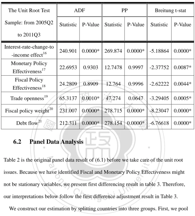
(37) Table2. Unit Root Test Result for variables in (6.1). The Unit Root Test. ADF. Sample: from 2005Q2. PP. Breitung t-stat. Statistic P-Value Statistic P-Value. Statistic. P-Value. to 2011Q3 Interest-rate-change-to -income effect16. 240.901 0.0000* 269.874 0.0000* -5.18864 0.0000*. Monetary Policy Effectiveness17. 22.6953. 0.9303. 12.7478. 0.9997. -2.37752 0.0087*. Fiscal Policy Effectiveness18. 24.2809. 0.8909. 12.764. 0.9996. -2.62222 0.0044*. 47.274 0.0647 政治大. -3.29405 0.0005*. Trade openness19. 65.3137 0.0010*. 立. 231.007 0.0000* 278.715 0.0000* -8.23047 0.0000*. Debt flow21. 212.311 0.0000* 278.154 0.0000* -6.76618 0.0000*. ‧ 國. Panel Data Analysis. ‧. 6.2. 學. Fiscal policy weight20. Nat. sit. y. Table 2 is the original panel data result of (6.1) before we take care of the unit root. n. al. er. io. issues. Because we have identified Fiscal and Monetary Policy Effectiveness might. i n U. v. not be stationary variables, we present first differencing result in table 3. Therefore,. Ch. engchi. our interpretations below follow the first difference adjustment result in Table 3. We construct our estimation by splitting countries into three groups. First, we pool all 17 countries together, with 398 samples. According to our previous results, most countries have positive Interest- Rate-Change-to-Income Effect. Under the 16. w As stated in (4.6), Interest-Rate-Change-to-Income Effect is defined as how much unit of income (Y) will be affected by a unit change in interest rate (Rf). 17. Monetary policy effectiveness is the elasticity of IS, calculated as. 18. The elasticity of LM is. 19. Trade openness is the proportion of the sum of import and export to GDP. Fiscal policy weight is calculated as .. 20 21. .. Debt flow is the proportion of additional increase of debt in the calculated quarter to GDP. 30.

(38) assumption of procyclicality capital requirement, the significance of trade flow indicates that countries with high trade flow relative to its GDP are tend to require larger adjustment to its capital requirement rule. To think intuitively, high trade-flow countries have higher dependency on other countries, thus the economic situation is more relative to others, especially in crisis. In order to prevent the spillover effects, more flexible capital requirement is needed22. In the second column, we have excluded six small countries which we consider extreme values, including Cyprus, Estonia, Luxemburg, Malta, Slovakia, and Slovenia. The results are similar with the. 政治大 the overall trend of our data. Finally, we pool only the 5 in-debt countries, including 立 previous panel, indicating that extreme values in the 6 small countries do not affect. Greece, Ireland, Spain, Portugal and Italy. The significance of expansionary policy. ‧ 國. 學. weight and effectiveness shows under pro-cyclical capital requirement, the more. ‧. weight and more effective fiscal policy is, the less capital requirement adjustment. sit. y. Nat. needed. In some point, this can be linked to the fact that countries with more. io. er. government expenditure should loosen capital requirements during recession but has an upper limit, i.e. the degree of loosen capital regulation should not be out of control,. al. n. v i n preventing these countries to goC into further break down. h e n g c h i U Besides, though not obvious in other countries, debt flow is significant when we pool the 5 countries together. The result indicates the higher the debt level, the higher level of capital requirement adjustment is needed. Last but not the least, the trade openness is not significant in these 5 countries. We interpret it as though trade openness play a part in determining capital requirement policy, other indicators, such as debt increase level in PIIGS countries have dominated trade openness. Therefore, for PIIGS, the capital requirement policy should be adjusted depending on the fiscal policy weight and. 22. For more detailed explanation to the relation between Interest-Rate-Change-to-Income-Effect, see footnote 15. 31.

(39) effectiveness, debt increase level in each quarter.. Table3. Panel Estimation Result for Variables in (6.1) Before First differencing. Dependant Variable:. All 17 countries. Interest-Rate-Changeto-Income Effect. excluding 6 small. 5 in-debt countries. countries. Sample: from 2005Q2 to. Coefficient P-Value Coefficient P-Value Coefficient P-Value. 2011Q3 Monetary Policy Effectiveness. -235984.5. -98499.8. 0.0000*. 0.0060*. 120275.7. 0.0000*. -52.16518. 0.0001*. -61.3473. 0.0028*. -51.743. 0.0031*. Fiscal Policy Weight. -2637.831. 0.2653. -2267.12. 0.4789. 5292.276. 0.0353*. Debt Flow. -7194.699. 0.2856. -7623.28. 0.3542. -8538.43. 0.1958. 128. 0.046948. 0.061236. sit. y. 276. 0.043851 a l 0.037293 v i n Ch 0.001281 0.004214 engchi U. n. F-Statistic Probabilities. io. Adjusted R-square. 398. er. R-square. Nat. Samples. ‧. ‧ 國. Trade Openness. -84754.8. 學. 政治大 1902.619 0.0094* 90630.28 立. 0.0091*. Fiscal Policy Effectiveness. 0.1572. 0.253382 0.22271 0.000001. Table4 Panel Estimation Result for Variables in (6.1) After First differencing. Dependant Variable:. All 17 countries. excluding 6 small. Interest-Rate-Changeto-Income Effect Sample: from 2005Q2 to. 5 in-debt countries. countries. Coefficient P-Value. Coefficient. P-Value. Coefficient P-Value. -154187.3. 0.2980. -215478.2. 2011Q3 Monetary Policy Effectiveness. 24143.14. 0.6974. 32. 0.0932.

(40) Dependant Variable:. All 17 countries. excluding 6 small. Interest-Rate-Changeto-Income Effect. 5 in-debt countries. countries. Sample: from 2005Q2 to Coefficient P-Value. Coefficient. P-Value. Coefficient P-Value. 2011Q3 Fiscal Policy Effectiveness. 2458.784. 0.4181. 163814.3. 0.1781. 223308.8. 0.0620*. Trade Openness. -18.2393. 0.0550*. -43.06878. 0.0129*. -17.19854. 0.2970. Debt Flow. -6341.946. 0.3060. -7000.504. 0.3278. -15316.68. 0.0308*. Samples. 398. R-square. 0.046948. 128. 政治 0.061236 大. 0.126240. 0.043851. 0.0889. 0.001281. 0.004214. 0.000001. F-Statistic Probabilities. 學. 立0.037293. Forecasting and Future Policy Suggestion. Nat. sit. y. ‧. ‧ 國. Adjusted R-square. 6.3. 276. io. er. In this section, we want to use the estimation result in previous section to forecast. al. v i n first differencing in figure 4 andC after in figure 5. Our result shows h efirstn differencing gchi U n. Interest- Rate-Change-to-Income Effect in 2012. We present the forecast result before. that most countries exhibit positive Interest- Rate-Change-to-Income Effect. After dealing with unit root by first differencing, Interest- Rate-Change-to-Income Effects in all the countries are positive. This indicates that in 2012, where the European Sovereign debt crisis deepens, counter-cyclical capital requirement should be adopted. Countries with decreasing GDP need loose capital requirement to inject revival to their economy. This is especially true in PIIGS countries. According to our previous analysis, the higher the value of Interest- Rate-Change-to-Income Effects, the less capital requirement adjustment needed to make. Observing from figure 4 and figure 5, 33.

(41) we find that among PIIGS, Greece, Italy, Spain and Portugal all have relative high value of Interest- Rate-Change-to-Income Effect. We conclude that instead of austerity measure, the authority should adopt counter-cyclical capital requirement. When recessions occur, the authority should loosen capital requirement but still holds an upper-limit to prevent further break down.. This also applies to other major Euro. Zone countries, such as Germany and France. However, for Ireland the result is different. It still shows Ireland need to loosen capital requirement in 2012 since it has encountered economic recession, and the lower value of Interest-Rate-to-Income. 政治大. Effect means Ireland should further decrease capital requirement since its GDP has declined in 2012.. 立. ‧. ‧ 國. 學. n. er. io. sit. y. Nat. al. Ch. engchi. 34. i n U. v.

(42) Forecast 2012 Interest-Rate-to-Income-Effect(1) 8000 6000 4000 2000 0 -2000 -4000 -6000 Ireland Slovakia h'. -3773. Malta. Estonia. Luxembo Netherla Slovenia Belgium Austria Germany Finland urg nds. Spain. Greece. Italy. Portugal France. 政治大 Forecast of 2012 Interest-Rate-Change-to-Income-Effect Before First differencing 立. -1066.5 -729.57 -2.9036 158.961 197.317 740.242 976.898 3013.54 3976.04 4445.31 4528.73 4779.16 5629.5 5906.27 6582.82. 學. ‧ 國. Figure4. n. al. er. io. sit. y. Nat. 7000 6000 5000 4000 3000 2000 1000 0. ‧. Forecast 2012 Interest-Rate-to-Income-Effect(2). Malta H' 1528.17. Slovakia Ireland 1880. Estonia. Ch. engchi. Netherla Belgium Slovenia Austria Germany Finland nds. 1988.25 2088.41 2384.83 2505.36 2614.67 3037.4. Figure5. i n U. v. Spain. Italy. France. Greece Portugal. 3515.5 3678.23 4061.09 4070.53 4355.53 4378.56 4789.91 5721.76. Forecast of 2012 Interest-Rate-Change-to-Income-Effect After First differencing. 35. Luxembo urg.

(43) 7 Conclusion In this paper, we followed the framework of Len-Kuo Hu (2012) to derive capital requirement strategies. Depending on interaction with liquidity shock, the loan’s project’s return, and the moral hazard problem, we derive the optimal capital requirement function, which determines on general economic condition in each country. Our model suggests that counter-cyclical capital requirement should be adopted when a country’s GDP is negatively related with its interest rate. On the. 政治大 when a country’s GDP is positively 立 related with its interest rate. With Keynesian's. contrary, the government should implement a pro-cyclical capital requirement policy. ‧ 國. 學. IS-LM framework, we are able to further specify how to identify whether capital requirement should increase or decrease as GDP changes.. ‧. We use the result of our model to test the optimal capital requirement strategies. sit. y. Nat. under the theme of ongoing European debt crisis. Our results can be summarized as. n. al. er. io. following. First, among the 17 countries across Euro Zone, most countries exhibit. i n U. v. positive relation between GDP and interest rate during 2005Q2 to 2011Q3, indicating. Ch. engchi. counter-cyclical capital requirement strategies should be adopted. Besides, in 2011, GDP in Greece, Ireland, Italy, Spain and Portugal are declining, meaning that these countries need loose capital requirement to foster its economic demands. The austerity measure will only worsen the already weak economic condition. Third, by constructing panel data, the result indicates that under the counter-cyclical capital requirement strategies, countries involved with higher trade are required to adopt more flexible capital requirement policy. When we only estimate PIIGS countries, the result shows that debt increase, fiscal policy weight and effectiveness dominate Interest- Rate-Change-to-Income Effects. Finally, when we use our data and equation 36.

(44) estimation result to forecast Interest- Rate-Change-to-Income Effects in 2012, we find all 17 Euro Zone countries should adopt counter-cyclical capital requirement policies. In addition, Greece, Italy, Portugal, France, and Spain are the countries needed to have an upper-limit when loosen capital requirement is adopted.. 立. 政治大. ‧. ‧ 國. 學. n. er. io. sit. y. Nat. al. Ch. engchi. 37. i n U. v.

(45) Appendix A: Detail Definition of Variables. Variables. C. Definition. Household final consumption expenditure. Consists of expenditure incurred by residents household on individual consumption of goods and services, household payment to the product provided by the government. It also includes various kinds of imputed expenditure of which the imputed rent for services of owner-occupied housing (imputed rents). Household final consumption includes household expenditure made on the domestic territory by residents and inbound tourists, but excludes residents' expenditure made abroad.. 立. ‧ 國. 學. Gross Capital Formation consists of outlays on addition to the fixed assets of an economy and net changes in inventories. Fixed asset includes land improvements, plant, machinery, equipment purchase, construction of the roads,. ‧. Gross Capital Formation (GFCF). y. io. sit. Nat. railways, schools, offices, hospitals, private residential dwellings, and commercial and industrial buildings. Inventories are stocks of goods held by firms to meet temporary or unexpected fluctuations in production or sales. Net acquisitions of valuables are also considered capital formation.. n. al. er. I. 政治大. G1. Government final consumption expenditure (GFCE). Ch. engchi. i n U. v. Government expenditure on goods and services that are used for the direct satisfaction of individual needs (individual consumption) or collective needs of members of the community (collective consumption). It mainly consists of the current expenditure, which is the sum of service and goods purchased by government, social payments and compensation to government employees.. G2. Total expenditure. The sum of current expenditure and capital expenditure. 1. Current expenditure The sum of compensation to government employees, the service and goods purchased by government, interests, social payments (social benefits and pensions paid in 38.

(46) money, and service funded by government that are produced and delivered to household by market units), and subsidies. 2. Capital expenditure The sum of government investment which deals with the acquisition of fixed capital asset, capital transfers, acquisition of stocks, valuable lands less the disposal of such asset. T. Sum of current revenue and capital revenue. 1. Current revenue The sum of direct taxes payable by household and. Tax. cooperation, indirect taxes which received by EU institutions, social contributions of employers and employees, sales which includes output for own final use as. 政治大 well as actual receipts from the sale of goods and services 立 by government units, receives of other current transfers.. ‧ 國. 學. ‧. Exports of goods and services represent the value of all. y. Nat. and service. goods and other market services provided to the rest of the world. They include the value of merchandise, freight, insurance, transport, travel, royalties, license fees, and other services, such as communication, construction, financial, information, business, personal, and government services. They exclude compensation of employees, investment income and transfer payments.. io. sit. Exports of goods. n. al. er. X. 2. Capital revenue The sum of capital taxes, investment grants and other capital transfers.. M. Imports of goods and service. Ch. engchi. i n U. v. Imports of goods consists the value of all goods and other market services received from the rest of the world. They include the value of merchandise, freight, insurance, transport, travel, royalties, license fees, and other services, such as communication, construction, financial, information, business, personal, and government services. They exclude compensation of employees, investment income and transfer payments. M2. Money Supply. M2 is defined as M1, which is the sum of currency in circulation and overnight deposit, plus deposits with an agreed maturity up to 2 years, and Deposits redeemable at a 39.

(47) period of notice up to 3 months. P. Harmonized Consumer Price Index(HICP). Rf. 3-month. Each country in European Union computes some 80 prescribed sub-indices, and their weighted average constitutes the national HICP. All countries uses 2005 as base period. The rate of interest rate charged on 3-month loans between banks.. Interbank rate. 立. 政治大. ‧. ‧ 國. 學. n. er. io. sit. y. Nat. al. Ch. engchi. 40. i n U. v.

(48) 2007Q1. 2007Q2. 2007Q3. 2007Q4. 2008Q1. 2008Q2. y. 2006Q4. 232. 54718. 4086. -232. 1540. 2790. -1571. 501. 192. 4906. 250. 1060. 6257. -10365. -334. -25. 1181. 43149. 4512. 30162. 2094. 1632. 71062. -336. 1652. 701. 10430. 4917. 472. 1742. 3589. -441. -304. 290. 910. 9732. 4221. 338. 1614. 4017. 2635. -887. 902. 5440. 2078 -118 4953. -179. 13855. 946. 92. 647. n i o10189. sit. 2006Q3. 231. 1167. 1226. 632. er. 2006Q2. 196. 2006Q1. 119. 2005Q4. 192. 2005Q3. 218. 2005Q2. 51. 401. 414. 152. 261. 234. 1232. 155. 431. Sloveni. -34368. -1292. 2094. NA. 264. NA. -5591. NA. -211. NA. 2453. a Slovaki. -2. -34. 12. -8. -8. -21. 26. -6. -16. -25. 829. -6. -10. ‧. 0. a Melta 388. 65. -141. 484. 823. -822. 2829. 271. 1207. -1936. -46703. 93165. Luxem. NA. 15. NA. NA. NA. NA. NA. NA. NA. NA. NA. NA. NA. -125. 2556. 938. engchi. Ch. 41. v i n U. al. 學. burg Estonia. -18. NA. 0. 162. NA. 125. -103. 1453. -68. -60. 626. 779. 203. -22. -27. 5521. 1198. 693. 655. 359. -50 18743. -167. 1164. 811. 176. Cyprus -831. -10703. -153. 178. 9702. -347. 310 574. -226. 47. 12664. 617. 7806 1175 1285. 732. 111535. N1833a t. 721. Netherl 1737 1506. 411. -2624. 1279. -83. 512. ands Finland -352 -176. 6292. 3438. 1517. 422. 4131. 983. Austia 69 16285. 1227. 857. 310. 5081. 3947. Belgiu 113432. 3889. 1637. -602. 3743. 19167. 956. m Germa 2723. 1196. -3665. 4803. 16199. -382. ny France 5430. 197. 4254. 12196. 981. Ireland. 273. 4753. 8375. -25205. Portuga. 4204. 14541. 774. 立. 政治大 1077. 6425. l Spain. 2993 -717. -3461 958. Italy Greece. ‧ 國. Appendix B: Value of Interest-Rate-to-Income Effect in 17 Euro Zone Country.

(49) 2011Q1. 2011Q2. 2011Q3. er. y. sit. 2010Q4. 2009Q4. 2010Q3. 2009Q3. 2010Q2. 2009Q2. 2010Q1. 2009Q1. -593. 2008Q4. 221. 2008Q3. 226. 220. 239. 3. 415. 320. 170. 219. 244. 212. 468. 167. 276. -951. 111. 732. 2083. 379. 709. 529. -53. 801. 434. 27. 7. 71. NA. -9. 21. NA. -17. 65. NA. NA. -7. 23. NA. 936. 972. -14. 32. NA. 629. 837. 4925. 132. 55 NA. 1724. 1247. 386. 275. 16416. NA. 869. 859. 938. -235. 833. 203. 893. 994. 636. 652. 1408. -803. 997. -1182. -742. 4952. ‧ 國. 3022. 15359 -13 n io N a t571 1806. 14112. 4321. -1888. 3707. 8042. 4633. 288. 1718. 2426. 4482. 265. 519. 8662. 4706. -316. 1836. 1276. 1941. 854. -1105. 457. 1531. 14442. ‧. -437. 45091. 4730 738 1877 296 4780 26794 438. 2245. 67982. -704. 學. 398. -20. 439. 52 NA. -14. 30 NA 966. -13. 49 NA -16 1200. -9. 103 NA 1305 1037 387. -15. NA 636 1158 3730 -448. -8. 230 8254 538 -302. 9127. -27. 842 218 -660 -51267. 5717. -15. 414 -805 7491 4254. 1848. -17. -313 5299 -1646. 1956. -1804. -95. -1221 2517 1586. 300. 4495. 4163. 25365 941 397. 4577. -3264. -810. 1908 185. 4824. 269. 767. 2573. 242 3970. 7432. 1047. 2154. 5083. -8818. 559. engchi 13442. 4481. 118. 1797. NA. NA. 4356. 4812. 361. 1660. NA. NA. 361. 716. NA. 1546. 3605. 381. 1746. NA. NA. 116. 1767. -1947. 962. -494. NA. al. 42. v. Ch. 548. 9925. 1069. 立. i n U. 78. 8386. 政治大.

(50) Appendix C: Descriptive Analysis of Raw Data In appendix C, we will have a brief look at the raw data, including GDP, cumulative level, trade openness, and policy weight and effectiveness to form big pictures of 17 countries.. C.1 GDP Across all 17 countries, we observe that the biggest scale economy is Germany, following France, Italy, Spain, and Netherlands. Countries with medium-sized GDP. 政治大 countries are Slovakia, Luxemburg, Slovenia, Cyprus, Estonia, and Malta. 立. are Belgium, Austria, Greece, Finland, Portugal and Ireland. The smallest-sized GDP 23. During. 2005Q1 to 2011Q3, we observe that all the countries have experienced economic. ‧ 國. 學. downturn during 2009, which leads to decrease in GDP. Almost all countries have. ‧. returned to its previous GDP except Greece, Ireland. This observation indicates that. sit. y. Nat. the economic situation in these two countries is deteriorating. Besides, although the. io. er. GDP once return to previous level, Italy, Spain, and Portugal are again experiencing recession with its GDP is falling in 2011.. n. al. Ch. engchi. 43. i n U. v.